Object-Based Crop Classification with Landsat-MODIS Enhanced Time-Series Data

Abstract

Cropland mapping via remote sensing can provide crucial information for agri-ecological studies. Time series of remote sensing imagery is particularly useful for agricultural land classification. This study investigated the synergistic use of feature selection, Object-Based Image Analysis (OBIA) segmentation and decision tree classification for cropland mapping using a finer temporal-resolution Landsat-MODIS Enhanced time series in 2007. The enhanced time series extracted 26 layers of Normalized Difference Vegetation Index (NDVI) and five NDVI Time Series Indices (TSI) in a subset of agricultural land of Southwest Missouri. A feature selection procedure using the Stepwise Discriminant Analysis (SDA) was performed, and 10 optimal features were selected as input data for OBIA segmentation, with an optimal scale parameter obtained by quantification assessment of topological and geometric object differences. Using the segmented metrics in a decision tree classifier, an overall classification accuracy of 90.87% was achieved. Our study highlights the advantage of OBIA segmentation and classification in reducing noise from in-field heterogeneity and spectral variation. The crop classification map produced at 30 m resolution provides spatial distributions of annual and perennial crops, which are valuable for agricultural monitoring and environmental assessment studies.

1. Introduction

Land use and land cover change is a primary driver of environmental change on Earth’s surface, and have significant implications on ecosystem health and sustainable land management [1]. Changes in global agricultural land use have been particularly widespread due to increasing population and consumption [2]. Agricultural expansion has had tremendous impacts on habitats, biodiversity, carbon storage, and soil conditions [3,4]. Detailed and up-to-date agricultural land use information is important to understand environmental impacts of cropping activities. Analysis of remotely-sensed imagery is a reliable and cost-effective method for crop monitoring across large areas and could provide consistent temporal records [5,6].

Frequent observations of remote sensing images can reveal unique characteristics of crops during their development cycles and, therefore, are particularly useful for agricultural land classification. Temporal trajectories were developed for warm season grassland mapping in tallgrass prairies using five images acquired by the Advanced Spaceborne Thermal Emission and Reflection Radiometer (ASTER) imagery [7]. The Landsat imagery with a 30 m spatial resolution was also found well suited for crop classification. For example, thirty-six Landsat images obtained from 2002 to 2005 were applied to extract temporal signatures of six main Mediterranean crops [8]. Time series of eight Landsat images were used to identify four main classes (bare soils, annual vegetation, trees on bare soil, and trees on annual understory) [9].

However, the 16-day revisit cycle of Landsat imagery limits the size of satellite time series, especially in crops’ growing season that is often associated with high cloud cover and precipitation [10]. In contrast, the Moderate Resolution Imaging Spectroradiometer (MODIS) has the capacity of daily observation and its products have spatial resolutions of 250 m, 500 m, and 1000 m. MODIS time series have been used to analyze crop phenological changes and to discriminate vegetation types at regional and global scales [11,12,13,14]. The eight-day, 500-m MODIS Normalized Difference Vegetation Index (NDVI) time series in a yearly span were used for the study of C3 and C4 grass plant functional types in different floristic regions [13]. With similar data sets, major annual (corn, soybean, winter wheat, and spring wheat) and perennial (shortgrass, warm-season tallgrass, and cool-season tallgrass) crops were mapped to assess the bioenergy-driven agricultural land use change in the U.S. Midwest [14]. However, at 250–1000 m resolution, a MODIS pixel often covers multiple crop fields on the ground. Small crop fields are lost and the accuracies of crop mapping were reduced at such coarse resolution [13].

To simulate reflectance data at higher resolutions in both spatial and temporal dimension, a Spatial and Temporal Adaptive Reflectance Fusion Model (STARFM) was developed to integrate TM and MODIS data for predicting daily surface reflectance at Landsat spatial resolution [15]. STARFM is perhaps the most widely-used data fusion algorithm for Landsat and MODIS imagery [16], which can result in synthetic Landsat-like surface reflectance [17,18]. An Enhanced Spatial and Temporal Adaptive Reflectance Fusion Model (ESTARFM) was developed based on the existing STARFM algorithm [19]. The most significant improvement of the ESTARFM is using a conversion coefficient to enhance the accuracy of prediction for heterogeneous landscapes. This fusion method is particularly useful for detecting gradual changes over large land areas, such as phenology studies [10,15,20,21,22,23].

Pixel-level spectral heterogeneity in croplands is a common problem in image classification [24]. For a medium-resolution pixel, its spectral reflectance is affected by different crop species, cropping systems and management activities. To overcome this difficulty, the Object-Based Image Analysis (OBIA) has been increasingly implemented in remote-sensed image analysis [25]. Applications of the OBIA model to image classification consider the analysis of an “object in space” instead of a “pixel in space” [26]. The most common approach used to generate such objects is image segmentation, which subdivides an image into homogeneous regions by grouping pixels in accordance with pre-defined criteria of homogeneity and heterogeneity [27]. For each object created in a segmentation process, spectral, textural, morphologic, and contextual attributes are generated and later employed in image classification [25]. All pixels in the entire object are assigned to the same class to avoid the salt-and-pepper noises in pixel-based classification [5].

Not all features extracted from imagery are necessarily conducive to improving the segmentation and classification accuracy. The selection of appropriate image features is a crucial step in any image analysis process [28]. Several feature selection methods have been used in conjunction with OBIA, such as the Bhattacharyya distance [29], Jeffreys-Matusita distance [30], and genetic algorithm [31]. Selection of optimal features has also been successfully applied through the decision tree analysis [32,33,34,35]. Stepwise Discriminant Analysis (SDA) effectively selects the subset of variables and has been applied for reduction of data dimensionality [36,37,38]. In the Classification and Regression Trees (CART), optimal features are identified based on their relative importance to classification [39,40].

In this study, we tested the feasibility of Landsat-MODIS Enhanced time series in crop mapping via the synergistic use of feature selection, OBIA segmentation and decision tree classification. The study area is in Southwest Missouri where a total of 18 TM and eight MODIS layers were acquired from February to November of 2006–2008. With Landsat-MODIS Enhanced time series data and the OBIA classification, the crop classification map generated at 30 m resolution can be applied to agriculture monitoring and management activities in this region.

2. Materials and Methods

Object-based crop classification with Landsat-MODIS Enhanced time series data mainly consists of four steps, including (1) the construction of time-series data with the ESTARFM algorithm; (2) NDVI time-series feature analysis and selection; (3) extraction of image objects using an image segmentation algorithm and quality assessment; and (4) decision tree classification based on the image objects. The methodology is summarized in Figure 1.

Figure 1. Flow diagram of crop classification.

Figure 1. Flow diagram of crop classification.

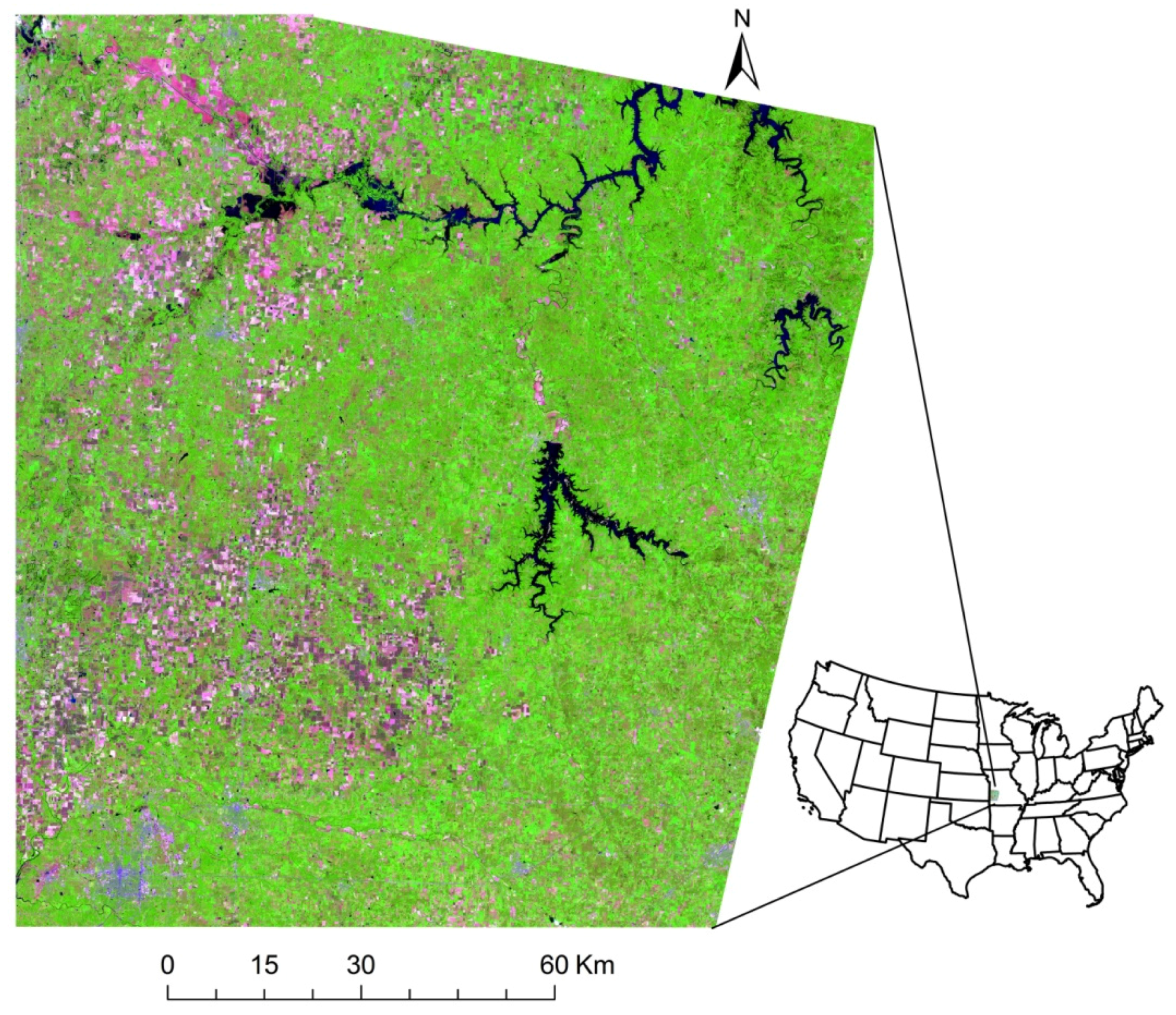
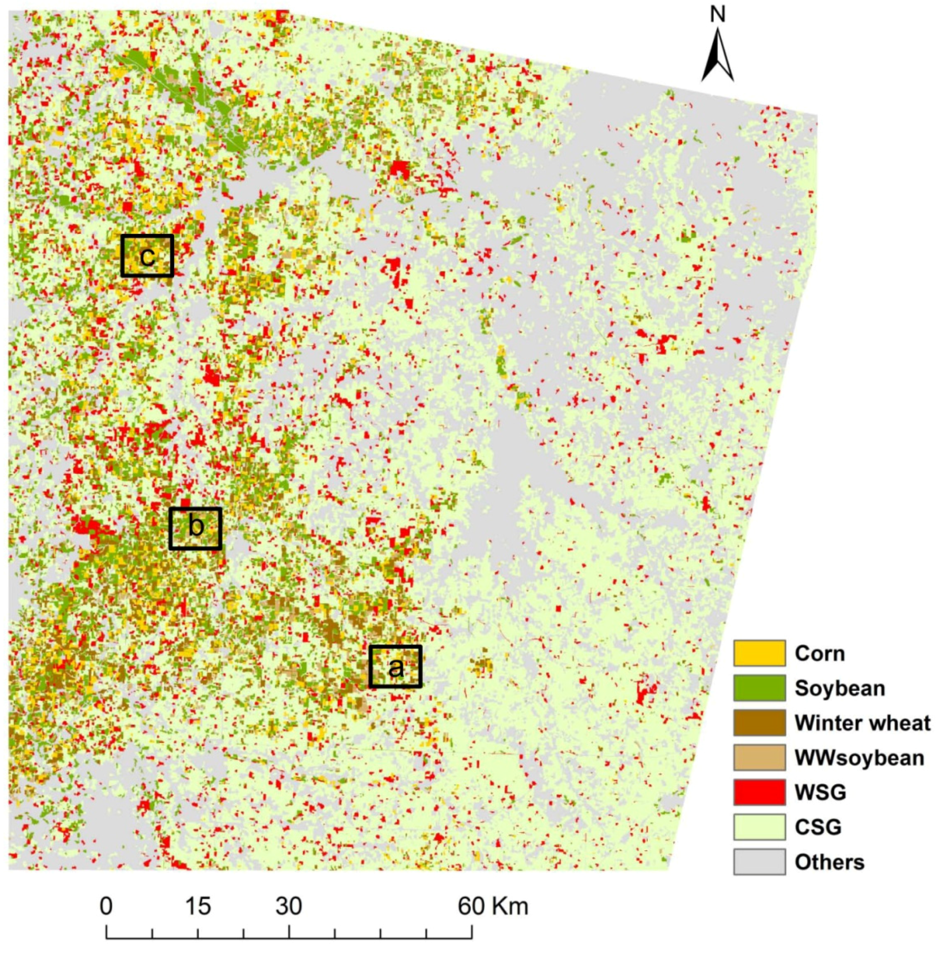
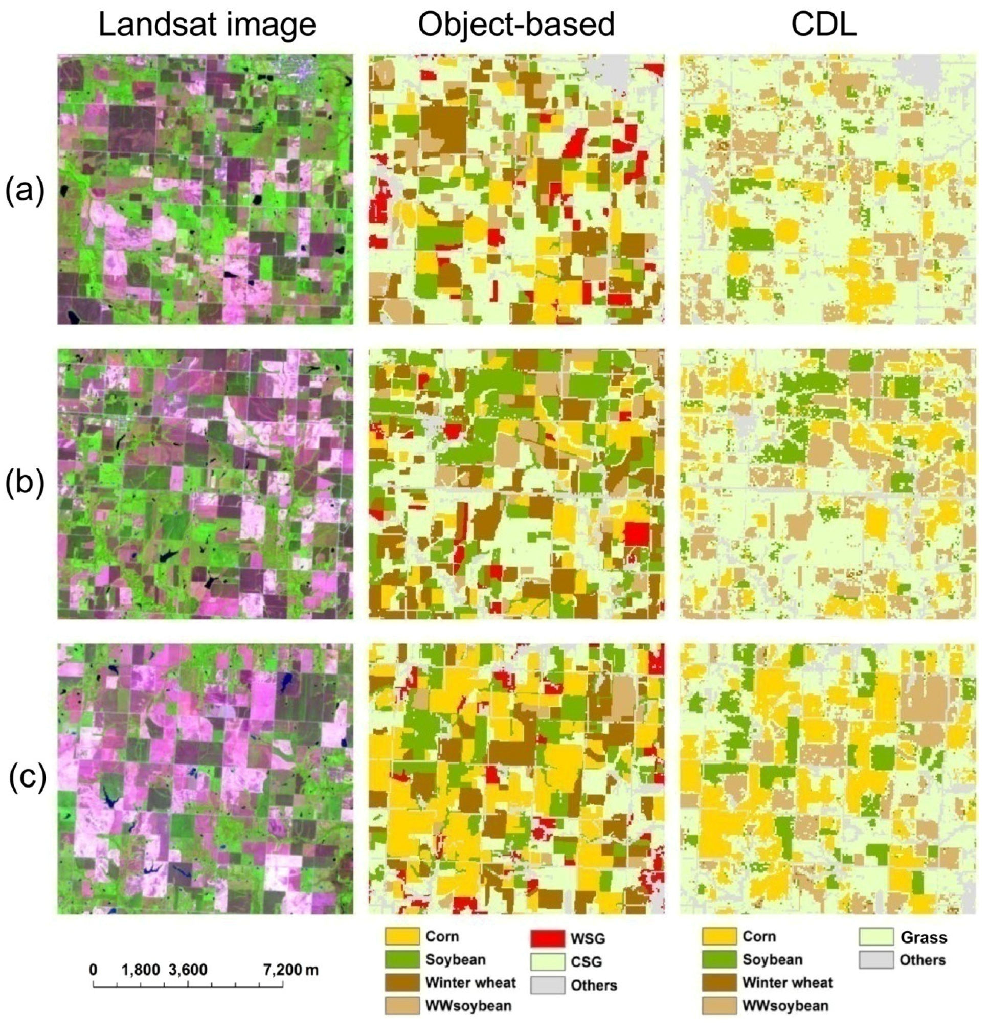
2.1. Study Area and Data Set

The study area was located in the lower Osage Plain in Southwest Missouri (Figure 2). In 2007, crop types in the study area were extracted in the Cropland Data Layer (CDL) product developed by National Agricultural Statistics Service (NASS), United States Department of Agriculture (USDA), using multi-temporal imagery acquired with the 56-m Indian ResourceSat-1 Advanced Wide Field Sensor (AWIFS) [41]. Major annual crops in the study area are corn, soybean, winter wheat, and winter wheat-soybean double cropping (WWSoybean). Cool-season grass (CSG) dominates the herbaceous pasture lands, while warm-season native prairie grass (WSG) remains in various prairie remnants that are often managed as recreational conservation areas [7]. Accuracy of the CDL data was around 85%–95% for major crop-specific land cover categories. Its accuracy in this grass-dominant study area is expected to be lower. The CSG and WSG are all classified as grass in CDL data. Non-crop lands (forests, water, urban development, etc.) were extracted from the 2007 CDL map and masked out in this study.

Figure 2. An example TM image of study area acquired on DOY 140, 2007 (R: band 5, G: band 4, B: band 3).

Figure 2. An example TM image of study area acquired on DOY 140, 2007 (R: band 5, G: band 4, B: band 3).

The study area is covered in one subset of Landsat image (path 26/row 34). In 2007 all TM images with low cloud covers were collected. In months when no good-quality TM images were available in 2007, those acquired in similar dates in 2006 and 2008 were used as an alternative. Although most of alternative images are acquired before or after the growing season (April to September) of crops, layer 16, 18, and 19 (5 August 2006, 21 August 2008, 6 September 2006) (Table 1) which are in the fall season may influence the crop classification due to the possible differences between years (farming procedures, crop types, hydrological conditions etc.). To reduce the influence of differences between years, the smoothing of NDVI time series and feature selection before classification were applied. A total of 18 TM images were collected, but the temporal gaps were still large in some months (Table 1). For example there is only one TM image available in May and one in July. The one-month interval of this series highly restricts the accuracy of crop mapping. When the temporal gaps between Landsat images in 2007 were larger than 16 days during growing season, the eight-day 500-m MODIS reflectance images (MOD09A1) were collected. The MOD09A1 products were used as our primary data source, as its time series have been proved to be useful in regional crop mapping [12,13,14]. Compared to MOD09Q1 (250-m), the MOD09A1 product contains a cloud mask layer, which makes its Maximum Value Composite (MVC)-resulted surface reflectance less affected by cloud in a spatial scale. The ESTARFM algorithm [19] was applied to disaggregate the MODIS images to 30-m pixel size. The algorithm is based on the premise that both Landsat and MODIS imagery observe the same reflectance, biased by a constant error. This error depends on the characteristics of a pixel, and is systematic over short temporal intervals. Therefore, if a base Landsat-MODIS image pair is available on the same date, this error can be calculated for each pixel in the image. These errors can then be applied to the MODIS imagery of a prediction date to obtain a Landsat-like prediction image on that date. All the images must be preprocessed to georegistered surface reflectance before implementing the ESTARFM [19]. In this study, the Landsat surface reflectance products we used were generated from the Landsat Ecosystem Disturbance Adaptive Processing System (LEDAPS) [42]. MODIS surface reflectance data were reprojected and resampled to the Landsat resolution using MODIS Reprojection Tools (MRT). LEDAPS uses similar atmospheric correction approach (6S approach) to the MODIS surface reflectance product. Therefore, reflectance from two sensors was consistent and comparable [42]. A 26-layer Landsat-MODIS time series with an average interval of approximately 10 days was produced for this study (Table 1).

Table 1. Time series of Landsat and MODIS fused images.

Number	Date	DOY	Number	Date	DOY
1	26 Februar 2006	057	14	7 July 2007	188
2	6 March 2007	065	15	20 July 2007M	201
3	14 March 2006	073	16	5 August 2006	217
4	2 April 2007	092	17	8 August 2007	220
5	7 April 2007M	097	18	21 August 2008	234
6	18 April 2007	108	19	6 September 2006	249
7	23 April 2007M	113	20	14 September 2007M	257
8	9 May 2007M	129	21	22 September 2007M	265
9	20 May 2007	140	22	29 September 2008	273
10	25 May 2007M	145	23	8 October 2006	281
11	2 June 2006	153	24	24 October 2006	297
12	10 June 2007M	161	25	30 October 2008	304
13	21 June 2007	172	26	9 November 2006	313

“M” that appears behind some dates represents MODIS and only MODIS data is available for the corresponding dates.

Table 1. Time series of Landsat and MODIS fused images.

Number	Date	DOY	Number	Date	DOY
1	26 Februar 2006	057	14	7 July 2007	188
2	6 March 2007	065	15	20 July 2007M	201
3	14 March 2006	073	16	5 August 2006	217
4	2 April 2007	092	17	8 August 2007	220
5	7 April 2007M	097	18	21 August 2008	234
6	18 April 2007	108	19	6 September 2006	249
7	23 April 2007M	113	20	14 September 2007M	257
8	9 May 2007M	129	21	22 September 2007M	265
9	20 May 2007	140	22	29 September 2008	273
10	25 May 2007M	145	23	8 October 2006	281
11	2 June 2006	153	24	24 October 2006	297
12	10 June 2007M	161	25	30 October 2008	304
13	21 June 2007	172	26	9 November 2006	313

“M” that appears behind some dates represents MODIS and only MODIS data is available for the corresponding dates.

The 2007 CDL map provided training and validation data for annual crops of corn, soybean, winter wheat, and WWSoybean. However, we found that the area of single-cropping winter wheat fields extracted by CDL was extremely small in the study area. The fall NDVI peaks during the soybean growth cycle of many WWSoybean fields were not obvious through visual interpretation, which indicated that some winter wheat fields were misclassified as WWSoybean. Therefore, we only selected pixels with apparent fall NDVI peaks as WWSoybean samples. The CDL product does not delineate WSG from CSG in herbaceous lands. In a published classification map from Wang et al. (2010), WSG and CSG were discriminated from ASTER images which provided reference samples for this study. A total of 1260 samples were selected (Table 2). The number of samples selected for each type of crops was proportional to its total area and uniformly distributed in the study area. The full datasets were randomly divided to training and validation subsets for the classification process. Table 2 lists the number of samples used for training and validation.

Table 2. The distribution of samples used for training and validation.

Crop Type	Training	Validation
Corn	155	83
Soybean	131	70
Winter wheat	134	72
WWSoybean	121	64
WSG	126	66
CSG	155	83
In total	822	438

Table 2. The distribution of samples used for training and validation.

Crop Type	Training	Validation
Corn	155	83
Soybean	131	70
Winter wheat	134	72
WWSoybean	121	64
WSG	126	66
CSG	155	83
In total	822	438

For assessment of segmentation quality, 108 samples were randomly selected from these 1260 samples. The boundaries of fields containing the 108 samples were interpreted with respect to the false color composite of TM image and also the high spatial resolution image in 2007 from Google Earth.

2.2. Feature Analysis and Selection

Spectral vegetation indices (VI), such as NDVI, have been widely used for analyzing and monitoring temporal and spatial variations of crop development [5,14]. In this study, NDVI features were used in crop field segmentation and classification. From the Landsat-MODIS Enhanced time series listed in Table 1, 26 layers of NDVI were calculated. The NDVI time series was smoothed with a five-point median filter followed by the 2nd-order polynomial Savitzky-Golay filter to reduce the atmospheric and cloud effects [13,14]. The average curve of each crop was retrieved by calculating the average NDVI of all training samples, which revealed crop growth cycle along the growing season (Figure 3).

The specific NDVI changing patterns of crops in Figure 3 indicate the feasibility of crop delineation with NDVI time series. Here we developed five NDVI Time Series Indices (TSI) based on their NDVI changing patterns along the growing season.

$$\text{TSI }1=\left(\text{NDVI }5-\text{NDVI }2\right)+\text{NDVI }6$$

(1)

$$\text{TSI }2=\left(\text{NDVI }11-\text{NDVI }6\right)+\left(\text{NDVI }12-\text{NDVI }8\right)$$

(2)

$$\text{TSI }3=\left(\text{NDVI }15-\text{NDVI }10\right)+\left(\text{NDVI }15-\text{NDVI }17\right)$$

(3)

$$\text{TSI }4=\left(\text{NDVI }12-\text{NDVI }5\right)+\text{NDVI }24$$

(4)

$$\text{TSI }5=\left(\text{NDVI }20-\text{NDVI }12\right)+\left(\text{NDVI }19+\text{NDVI}20\right)/2$$

(5)

TSI 1 reflects the change patterns of crops with early NDVI peak (winter wheat, WWsoybean, and CSG). TSI 2 reflects the change patterns of WSG. TSI 3 reflects the change patterns of corn. TSI 4 reflects the change patterns of CSG. TSI 5 reflects the change patterns of WWsoybean with its second NDVI peak in fall.

Optimal features were selected from the 31 features (26 NDVIs and five TSIs) to reduce data redundancy and inter correlation for crop segmentation and classification. The Stepwise Discriminant Analysis (SDA) was tested to select features by maximizing the variances among classes while minimizing the within-class variances. For the SDA technique, the Wilks’ Lambda testing was used which chooses entry variables into the equation and evaluates how much they lower Wilks’ lambda. At each step, the variable that minimizes the overall Wilks’ lambda is entered. The entry F value is 3.84 and removal F value is 2.71 to perform SDA in the Predictive Analytics Software and Solutions (SPSS) Statistics [43].

Figure 3. The average NDVI time series of six crops in the study area.

Figure 3. The average NDVI time series of six crops in the study area.

2.3. OBIA Segmentation and Quality Assessment

Image segmentation was completed using the multi-resolution segmentation algorithm in the commercial software Definiens eCognition Developer 8.0. The segmentation approach used in eCognition is a bottom-up region merging technique starting with one-pixel objects, and smaller objects are merged into larger ones in iterative steps [44]. The segmented outputs are controlled by a scale factor and a heterogeneity criterion. The scale factor determines the average size of resultant objects. The heterogeneity criterion includes two mutually exclusive properties: color and shape. Color refers to the spectral homogeneity. Shape considers the geometric/geomorphologic characteristics of objects, and is further divided into two equally exclusive properties: smoothness and compactness [44]. In general the segmentation process requires several user-specified parameters, including (1) the weights associated with input image layers; (2) a scale factor; (3) a color/shape ratio; and (4) a compactness/smoothness ratio [45].

Several scales (10, 15, 20, 30) were tested in image segmentation. At each scale, the segmented objects were visually checked with the corresponding crop field boundaries that could be easily interpreted in the image. Quality assessment was performed to identify the appropriate scale factor in this study. When a scale factor was set, the color and shape criteria were modified to refine the shape of the image objects. Previous studies found that more meaningful objects were extracted with a larger weight for color [38]. In this study the color was assigned with a weight of 0.7, whereas the shape received the remaining weight of 0.3. Both compactness and smoothness were assigned a weight of 0.5.

For purpose of quantitative assessment, several criteria have been developed to examine how the segmented polygons matched the original areas of interest, i.e., crop fields in this study. We applied the method by Möller et al. and Ke et al. [45,46] to evaluate image segmentation based on the topological and geometric similarities between segmented objects and reference objects. A total of 108 field polygons were used as reference objects that clearly delineate the boundaries of crop’s fields. Three metrics were calculated to represent the overall segmentation quality: (1) the relative area of an overlapped region to a reference object (${\text{RA}}_{\text{or}}$); (2) the relative area of an overlapped region to a segmented object (${\text{RA}}_{\text{os}}$); and (3) the position discrepancy of segmented object to a reference object (${\text{D}}_{\text{sr}}$), calculated as the average distance between centroids of segmented objects and the centroids of the reference objects.

$${\text{RA}}_{\text{or}}=\frac{1}{\text{n}}{\displaystyle \sum }_{\text{i}=1}^{\text{n}}\frac{{\text{A}}_{\text{o}}\left(\text{i}\right)}{{\text{A}}_{\text{r}}\left(\text{i}\right)}\times 100$$

(6)

$${\text{RA}}_{\text{os}}=\frac{1}{\text{n}}{\displaystyle \sum }_{\text{i}=1}^{\text{n}}\frac{{\text{A}}_{\text{o}}\left(\text{i}\right)}{{\text{A}}_{\text{s}}\left(\text{i}\right)}\times 100$$

(7)

$${\text{D}}_{\text{sr}}=\frac{1}{\text{n}}{\displaystyle \sum }_{\text{i}=1}^{\text{n}}\sqrt{{\left({\text{X}}_{\text{s}}\left(\text{i}\right)-{\text{X}}_{\text{r}}\left(\text{i}\right)\right)}^2+{\left({\text{Y}}_{\text{s}}\left(\text{i}\right)-{\text{Y}}_{\text{r}}\left(\text{i}\right)\right)}^2}$$

(8)

where n represents the number of segmented objects (n = 108 in this study), ${\text{A}}_{\text{o}}\left(\text{i}\right)$ is the area of the ith overlapped region associated with a segmented object and a reference object, ${\text{A}}_{\text{r}}\left(\text{i}\right)$ is the area of the reference object, ${\text{A}}_{\text{s}}\left(\text{i}\right)$ is the area of the ith segmented object; ${\text{X}}_{\text{s}}\left(\text{i}\right)$ and ${\text{Y}}_{\text{s}}\left(\text{i}\right)$ are the coordinates of the centroid of ith segmented object, and ${\text{X}}_{\text{r}}\left(\text{i}\right)$ and ${\text{Y}}_{\text{r}}\left(\text{i}\right)$ are the coordinates of the centroid of reference object.

${\text{RA}}_{\text{or}}$ and ${\text{RA}}_{\text{os}}$ were used to evaluate the topological similarity between segmented objects and reference objects. Values close to 100 indicate that reference objects are well segmented. The average distance ${\text{D}}_{\text{sr}}$, represents the positional accuracy of segmented objects. ${\text{D}}_{\text{sr}}$ of positionally accurate objects are close to 0, while both under-segmentation and over-segmentation increasing ${\text{D}}_{\text{sr}}$.

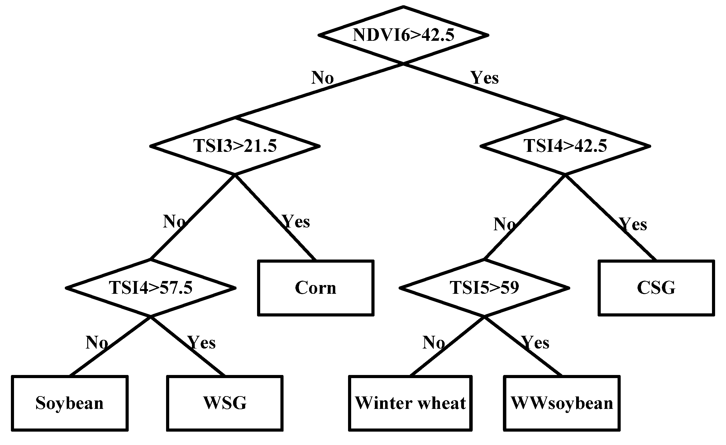
2.4. Decision Tree Classification

The object-based classification consists mainly of two steps: (1) delimitation of crop-fields by image segmentation; and (2) application of decision rules. After segmentation, a decision tree classification was applied to the OBIA metrics. As a non-parametric method, it requires no assumptions for data distribution and feature independency. The model design was conducted using a training/validation dataset. The training dataset was used to create, prune, and evaluate the decision trees, and the validation dataset was used to assess the accuracy of the image classification with the confusion matrix method [5,47,48].

The optimal features selected by SDA were used to build DT models for crop identification. The tree was built by binary recursive splitting of the training dataset, choosing the feature and the cutting value that best fit the partial response in every split. The cross-validation method was applied for the definition and evaluation of the models. A simple five-node DT was generated using training samples based on the selected features (Figure 4). Four features, namely NDVI 6, NDVI TSI 3, NDVI TSI 4, and NDVI TSI 5 which derived from nine dates of images were used in the DT. The DT classified each segmented object into one of the six crops in this study.

The coincidence between classified and ground-truth data was assessed at the field scale. The user’s and producer’s accuracies for each crop type and overall accuracy for the six crops were calculated. The object-based classification result was also visually compared with the CDL product in 2007.

Figure 4. The DT generated using training samples.

Figure 4. The DT generated using training samples.

3. Results

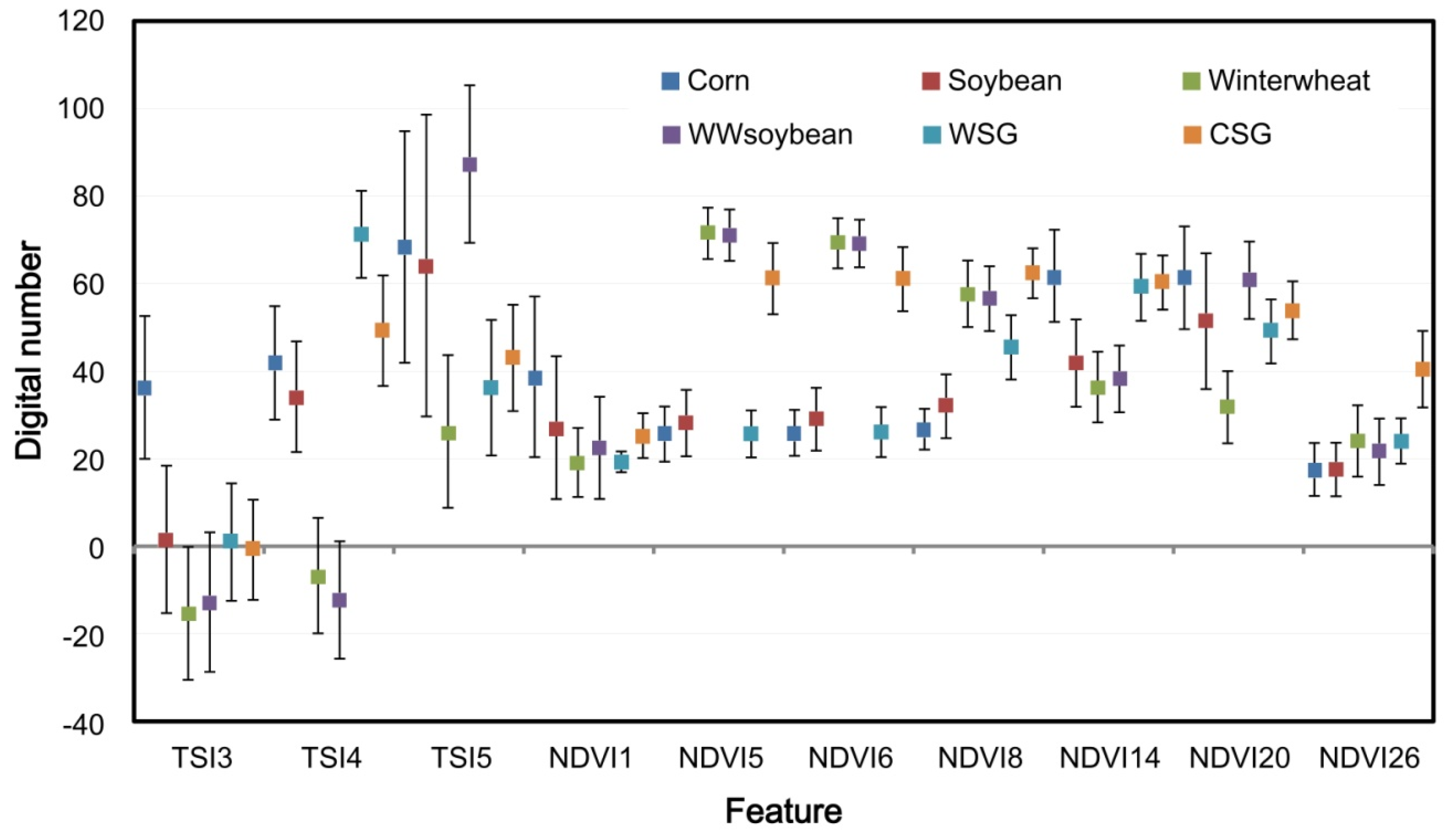
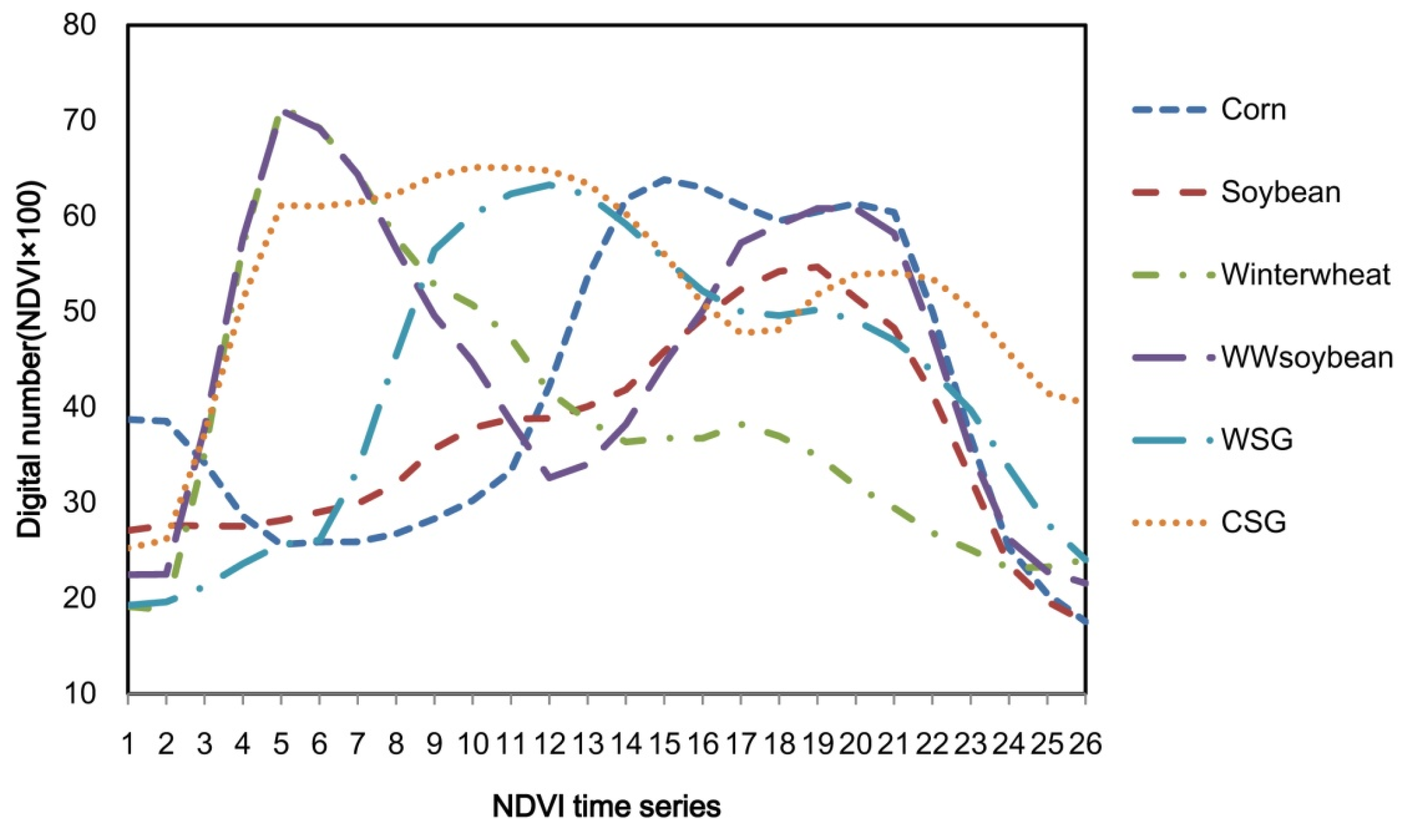
3.1. Feature Analysis and Selection

As shown in Figure 3, annual crops have shorter growth seasons than grasses. Corn was planted slightly earlier than soybean, but their curves were quite similar. Winter wheat was characterized with the earliest peak in NDVI (in April–May). The winter wheat-soybean (WWsoybean) double cropping had the earliest peak in NDVI in April–May and a second NDVI peak in fall. Cool-season grass (CSG) started its growth in early spring and reached peak growth in April to May, while warm-season grass (WSG) started in later spring and had delayed peak dates. In addition, CSG turned into dormancy in summer and has a second growth peak in fall, while WSG just remained green in summer.

Table 3 presents the F values of 31 features after 10 steps of SDA analysis. 10 features were selected (the first 10 features in Table 3) by SDA. Interestingly, three of five TSIs were selected, which suggests that the TSI features appeared to be informative for differentiating crop types. Those features selected by and SDA were selected as input features for image segmentation (highlighted in bold in Table 3). 13 images were used in the 10 selected features (seven NDVIs and three TSIs).

Means and standard deviations of training samples of the 10 selected features for six crop types are shown in Figure 5. NDVI 6 can split the samples into two groups (high NDVI and low NDVI). TSI 3 can separate corn from other crops because corn has high TSI 3 values while those of other crops are close to zero, or even negative. WSG has higher value of TSI 4 than corn and soybean and CSG has higher TSI 4 than winter wheat and WWsoybean. WWsoybean has higher TSI 5 than winter wheat. Therefore, it is reasonable that these four features were used in image segmentation and DT classification.

Table 3. F value of 31 features after 10 steps of SDA analysis.

Feature	Tolerance	F Value	Wilks‘ Lambda
NDVI TSI 4	0.234	23.636	0.005
NDVI 01	0.873	23.108	0.005
NDVI 08	0.516	18.644	0.004
NDVI 06	0.072	17.219	0.004
NDVI 20	0.04	10.918	0.004
NDVI 26	0.607	10.828	0.004
NDVI TSI 3	0.291	9.992	0.004
NDVI TSI 5	0.036	9.757	0.004
NDVI 14	0.212	6.904	0.004
NDVI 05	0.064	5.557	0.004
NDVI 09	0.077	3.831	0.004
NDVI 19	0.1	3.754	0.004
NDVI 13	0.038	3.428	0.004
NDVI 12	0.141	3.248	0.004
NDVI 24	0.219	3.248	0.004
NDVI 17	0.308	2.687	0.004
NDVI 25	0.082	2.649	0.004
NDVI 07	0.042	2.609	0.004
NDVI 22	0.258	2.607	0.004
NDVI 11	0.234	2.215	0.004
NDVI 16	0.322	2.164	0.004
NDVI 10	0.206	2.14	0.004
NDVI TSI 2	0.118	2.033	0.004
NDVI 21	0.114	1.919	0.004
NDVI 23	0.307	1.698	0.004
NDVI 15	0.109	1.243	0.004
NDVI TSI 1	0.019	1.111	0.004
NDVI 02	0.038	1.111	0.004
NDVI 03	0.125	0.964	0.004
NDVI 18	0.181	0.822	0.004
NDVI 04	0.122	0.627	0.004

Table 3. F value of 31 features after 10 steps of SDA analysis.

Feature	Tolerance	F Value	Wilks‘ Lambda
NDVI TSI 4	0.234	23.636	0.005
NDVI 01	0.873	23.108	0.005
NDVI 08	0.516	18.644	0.004
NDVI 06	0.072	17.219	0.004
NDVI 20	0.04	10.918	0.004
NDVI 26	0.607	10.828	0.004
NDVI TSI 3	0.291	9.992	0.004
NDVI TSI 5	0.036	9.757	0.004
NDVI 14	0.212	6.904	0.004
NDVI 05	0.064	5.557	0.004
NDVI 09	0.077	3.831	0.004
NDVI 19	0.1	3.754	0.004
NDVI 13	0.038	3.428	0.004
NDVI 12	0.141	3.248	0.004
NDVI 24	0.219	3.248	0.004
NDVI 17	0.308	2.687	0.004
NDVI 25	0.082	2.649	0.004
NDVI 07	0.042	2.609	0.004
NDVI 22	0.258	2.607	0.004
NDVI 11	0.234	2.215	0.004
NDVI 16	0.322	2.164	0.004
NDVI 10	0.206	2.14	0.004
NDVI TSI 2	0.118	2.033	0.004
NDVI 21	0.114	1.919	0.004
NDVI 23	0.307	1.698	0.004
NDVI 15	0.109	1.243	0.004
NDVI TSI 1	0.019	1.111	0.004
NDVI 02	0.038	1.111	0.004
NDVI 03	0.125	0.964	0.004
NDVI 18	0.181	0.822	0.004
NDVI 04	0.122	0.627	0.004

Figure 5. Means (square) and standard deviations (short line) of the 10 selected features. Calculated from the training samples of each crop.

Figure 5. Means (square) and standard deviations (short line) of the 10 selected features. Calculated from the training samples of each crop.

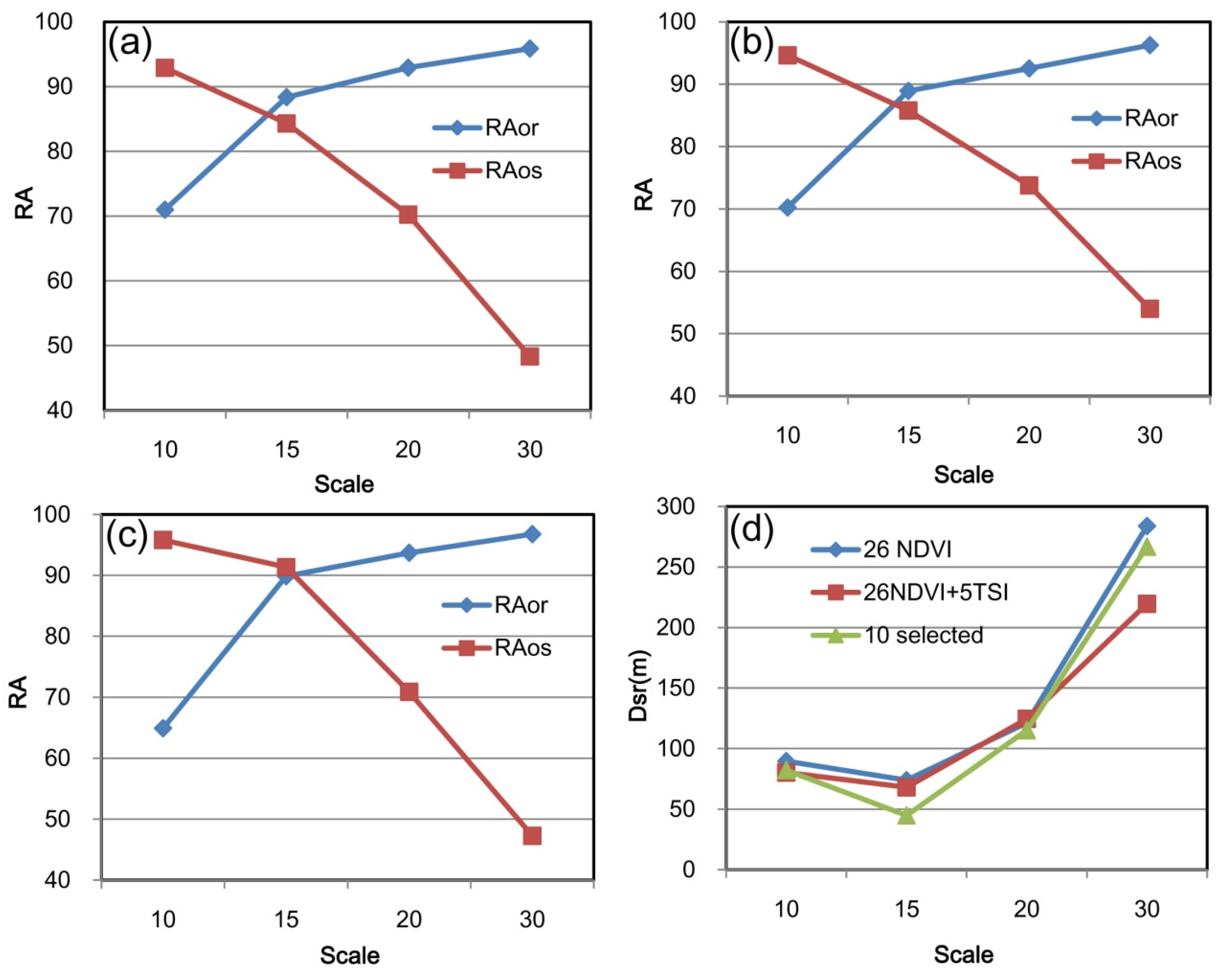
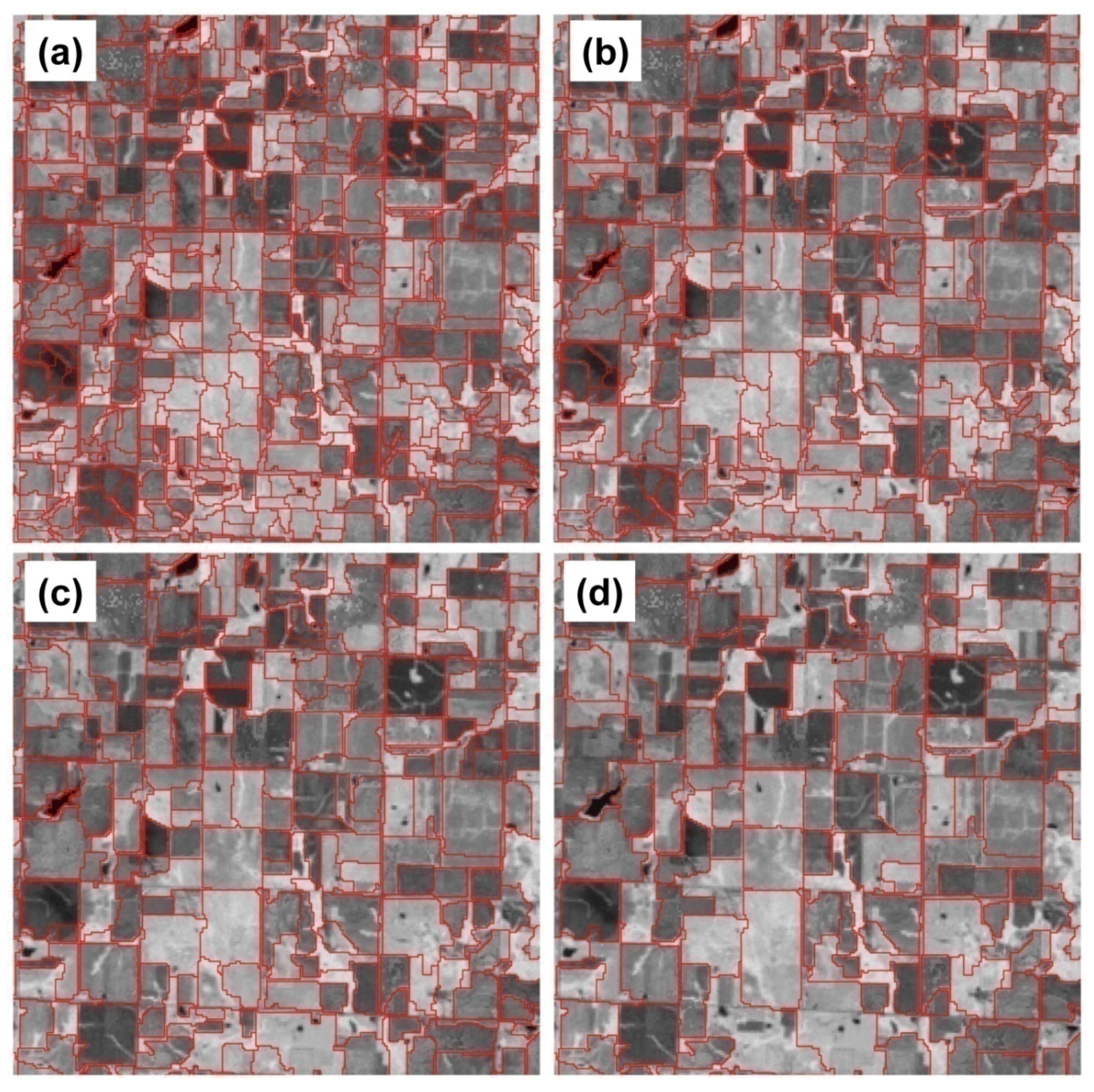
3.2. Image Segmentation and Quality Assessment

In Figure 6, similar patterns of ${\text{RA}}_{\text{or}}$ and ${\text{RA}}_{\text{os}}$ values are found in all three segmentation schemes (NDVI only, NDVI+TSI, and 10 optimal features), with increasing ${\text{RA}}_{\text{or}}$ and decreasing ${\text{RA}}_{\text{os}}$ from scale parameter 10 to 30. At a small scale (scale parameter 10), all three segmentations had low ${\text{RA}}_{\text{or}}$ values (e.g., 65% for segmentation from the 10 selected features) and high ${\text{RA}}_{\text{os}}$ values (e.g., 96% for segmentation from the 10 selected features). The low ${\text{RA}}_{\text{or}}$ and high ${\text{RA}}_{\text{os}}$ values of segmented objects of interest indicated over-segmentations at small scales. At large scales (scale parameter 20 and 30), the three segmentation schemes produced high ${\text{RA}}_{\text{or}}$ values, low ${\text{RA}}_{\text{os}}$ values of segmented objects that indicated under-segmentation.

For all segmentation schemes, similar ${\text{RA}}_{\text{or}}$ and ${\text{RA}}_{\text{os}}$ values were found at scale parameter 15. This similarity indicates the overall balance between over-segmentation and under-segmentation for the reference objects. Therefore, the scale parameter at 15 was used as the optimal scale for segmentation of crop fields. At this scale, a shape parameter of 0.3 and a compactness parameter of 0.5 were selected for image segmentation.

As shown in Figure 6, at scale parameter of 15, the ${\text{RA}}_{\text{or}}$ and ${\text{RA}}_{\text{os}}$ values from the segmentation with 10 selected features ${\text{RA}}_{\text{or}}$ = 90% and ${\text{RA}}_{\text{os}}$ = 91%) are much higher than those of the other two segmentation schemes. That meant that objects segmented from the 10 selected features had better match with reference objects than the other two schemes, revealing the necessity of feature selection for the image segmentation.

Figure 6. The segmentation quality assessment (a) RA of segmentation based on 26 NDVI; (b) RA of segmentation based on 26 NDVI + 5 NDVI TSI; (c) RA of segmentation based on the 10 selected features; and (d) the distance of centroid of segmented objects to centroid of reference objects (${\text{D}}_{\text{sr}}$).

Figure 6. The segmentation quality assessment (a) RA of segmentation based on 26 NDVI; (b) RA of segmentation based on 26 NDVI + 5 NDVI TSI; (c) RA of segmentation based on the 10 selected features; and (d) the distance of centroid of segmented objects to centroid of reference objects (${\text{D}}_{\text{sr}}$).

Positional accuracies of segmented objects are illustrated in Figure 6d. For all three segmentation schemes, the distance between the centroids of segmented objects and the centroids of reference objects decreased with increasing scales until a minimum was reached, then increased at larger scales. At small scales, over-segmentation produced multiple segments overlapping with a single reference object, which caused large ${\text{D}}_{\text{sr}}$ values. Under-segmentation, on the other hand, produced larger segments than reference objects, thus also resulted in increased ${\text{D}}_{\text{sr}}$ values. The minimum distance was produced at scale parameter 15 for all three segmentations. The ${\text{D}}_{\text{sr}}$ from the segmentation with 10 selected features had the smallest ${\text{D}}_{\text{sr}}$ at the scale parameter 15, which also meant that objects segmented from 10 selected features had better match with reference objects than other segmentation schemes.

The combination of topological accuracies (${\text{RA}}_{\text{or}}$ and ${\text{RA}}_{\text{os}}$) and positional accuracies (${\text{D}}_{\text{sr}}$) showed that the best resemblance of segmented objects to the reference objects was produced from the segmentation with 10 selected features at scale 15. Figure 7 demonstrates the segmented images of a subset at scale parameters 10, 15, 20, and 30, respectively. Visual interpretation was consistent with Figure 6 that the segmented objects around other scales were not aligned well with the crop field boundaries. The scale parameter of 10 was too small and the scale parameter of 20 was too large for the crop field segmentation.

Figure 7. Demonstration of image segmentation at four scale levels: (a) scale parameter 10; (b) scale parameter 15; (c) scale parameter 20; and (d) scale parameter 30.

Figure 7. Demonstration of image segmentation at four scale levels: (a) scale parameter 10; (b) scale parameter 15; (c) scale parameter 20; and (d) scale parameter 30.

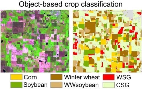
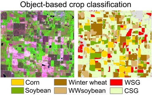
3.3. Crop Classification Using Object-Based Metrics

The DT classification shows detailed spatial distributions of the six crop types (Figure 8). Four crop types, corn, soybean, winter wheat and double cropping winter wheat-soybean are identified and mapped mainly in the west part of the image. Grasslands which are comprised of WSG and CSG are distributed in the east part of the image.

Accuracy assessment of the object-based classification was performed with validation samples listed in Table 2. According to Foody (2002), it is desirable for a classification to reach an accuracy higher than 85% [49]. As shown in the error matrix (Table 4), an overall accuracy of 90.87% and a kappa coefficient 0.89 indicate good quality of our classification. Specifically, the producer’s accuracy of WSG and CSG is higher than 95%, the producer’s accuracy of winter wheat is 94.44% and the producer’s accuracy of WWsoybean is 87.5%. However, the producer’s accuracy of corn and soybean is slightly lower (84.34% of corn and 84.29% of soybean) than other crops. The user’s accuracy of corn and soybean was also a little lower than other crops. 10.84% of corn was classified as soybean and 11.43% of soybean was classified as corn because their NDVI time series curves were quite similar. Some WWsoybean was misclassified as winter wheat.

Figure 8. The classification results using object-based method. Rectangles named (a), (b), and (c) are three subset areas for the demonstrative comparison between our classification and CDL product.

Figure 8. The classification results using object-based method. Rectangles named (a), (b), and (c) are three subset areas for the demonstrative comparison between our classification and CDL product.

Table 4. The error matrix for the object-based classifications (%).

Class	Reference
	Corn	Soybean	WW	WWsoy	WSG	CSG	UA
Corn	70	8	0	0	1	0	88.61
Soybean	9	59	0	0	2	0	84.29
WW	0	0	68	7	0	0	90.67
WWsoy	0	0	2	56	0	0	96.55
WSG	4	2	0	0	63	1	90.00
CSG	0	1	2	1	0	82	95.35
PA	84.34	84.29	94.44	87.5	95.45	98.80
OA	90.87
Kappa	89.02

UA: user’s accuracy (%); PA: producer’s accuracy (%); OA: overall accuracy.

Table 4. The error matrix for the object-based classifications (%).

Class	Reference
	Corn	Soybean	WW	WWsoy	WSG	CSG	UA
Corn	70	8	0	0	1	0	88.61
Soybean	9	59	0	0	2	0	84.29
WW	0	0	68	7	0	0	90.67
WWsoy	0	0	2	56	0	0	96.55
WSG	4	2	0	0	63	1	90.00
CSG	0	1	2	1	0	82	95.35
PA	84.34	84.29	94.44	87.5	95.45	98.80
OA	90.87
Kappa	89.02

UA: user’s accuracy (%); PA: producer’s accuracy (%); OA: overall accuracy.

In Figure 9, the object-based classification is visually compared with CDL product in three subsets of the study area (a, b, and c, with their locations shown in Figure 8). In our results, crop fields were discriminated better than CDL. Classification noises caused by in-field spectral variations were also removed. The winter wheat and WWsoybean were discriminated in he object-based result, but they were mixed and most of winter wheat was classified as WWsoybean in the CDL map. Superior to the CDL product, our classification delineated WSG from CSG grasses based on their asynchronous seasonality.

Figure 9. Demonstrative comparison between our classification and CDL products in three subsets of (a–c). Column (1) the color composite display R (band 5) G (band 4) B (band 3) of Landsat 5 image in DOY 140 of 2007; column (2) object-based classification map; and column (3) CDL map.

Figure 9. Demonstrative comparison between our classification and CDL products in three subsets of (a–c). Column (1) the color composite display R (band 5) G (band 4) B (band 3) of Landsat 5 image in DOY 140 of 2007; column (2) object-based classification map; and column (3) CDL map.

4. Discussion

This study confirmed the effectiveness of the object-based classifier technique for cropland classification from time series data [5,24]. The OBIA segmentation of images into homogenous parcels reduced with-in field variability and better-delineated field boundaries. The classification results demonstrates the potential of the objected-based approach to map crop areas using multi-temporal data.

Considering the work by Peña-Barragán et al. [5] and Vieira et al. [24], our study makes an important and distinct contribution, as we focused on the use of the dense time series data and feature selection method which demonstrates the key dates for crop classification. 26 images were collected and generated by the fusion of Landsat and MODIS data using the ESTARFM algorithm, which are more dense than three or four images of previous studies. 13 images were used in the segmentation and among them nine were used in the classification with DT. The dates of selected features mainly are the peak and inflection points of NDVI time series curves, for example NDVI 6 reflects the earliest peak NDVI of winter wheat in April. These dates are related to crop growth patterns. In particular, three TSIs were selected in the DT. The principle of NDVI TSIs is based on the difference of crops phenology and growth patterns, which reveals that the multi-temporal approach is essential to obtain high accuracy crops’ classification. These selected dates reflect the growing season period in which crops are more feasible to be discriminated. The optimal time periods of collecting satellite images not only improve the accuracy of segmentation and classification, but also reduce computational time of image analysis procedures, especially for the image segmentation which has high demand of computational resources.

The usage of the data from different years may cause problem due to the possible differences between years. However, it will not influence the classification result seriously in this study based on our analysis. For images acquired before or after the growing season, the NDVIs of all crops except CSG in fall are low and similar. The data acquired in these periods can be used as alternatives to 2007 data. The NDVIs of four crops (corn, soybean, winter wheat, and WWSoybean) are low and similar in early June, while the NDVIs of grass (WSG and CSG) are high. Comparing the CDL layer from 2006 to 2008, the conversion between grasslands and croplands was rare. The usage of layer 11 (2 June 2006) has little influence to the classification result. For layers of 16, 18, and 19 acquired in the fall season, the usage of data in 2006 and 2008 may influence the classification result. The smoothing of NDVI time series and feature selection before classification can reduce these influences to some degree. The 10 features which were selected for segmentation and classification used 13 images. Only 4 (NDVI 1, 19, 24, and 26) of the 13 images were not from 2007 and only one (NDVI 19, used in TSI 5) of them was in fall growing season.

Scale is one of the most critical factors that impact the quality of image segmentation. Scale parameter characterizes the spatial scale of segmentation because it is positively related to resultant object size. The optimal value of scale can be determined by the segmentation assessment as shown in Figure 6. In a general sense, the product of the optimum scale parameter (15) and spatial resolution (30 m) indicates the average object size of 450 m in length, which is fairly coincident with the average field size (20.5 ha) in the Midwest [50]. The size of optimal scale parameter may be equivalent to the real size of object.

While the OBIA classification approach produces reasonable results with efficiency, there are some limitations that should be considered in future research. Classification based on multi-scale segmentation often suffers from error propagation at the object level across different object scales [51]. The errors in the segmentation process of crop fields can result in uncertainties in the classification results. In addition, the similarity of NDVI time series curves of corn and soybean leads to their confusion, since corn is planted slightly earlier than soybean. Incorporation of textural features in the classification procedure could be considered to discriminate these crop types in further studies.

Results of this study provide supplementary information for national CDL products. The winter wheat single cropping and winter wheat-soybean double copping fields are better delineated based on earliest growing peak (NDVI 6) of winter wheat and fall NDVI TSI (TSI 5) of soybean, while these two classes in the CDL product are highly confused in the study area. In addition, this study provides the first map of perennial WSG grasses that have never been classified in published databases (e.g., CDL). As a supplement to CDL map, cropland classification derived in this study at 30 m resolution can provide valuable information for agricultural management and environment assessment research in this area and eventually to assist bioenergy policy-making at regional scale.

5. Conclusions

An integrative analysis of feature selection, Object-Based Image Analysis (OBIA) segmentation, and decision tree classifier was explored for crop classification from high temporal-resolution Landsat-MODIS Enhanced NDVI time series. Feature selection improved the accuracy of segmentation and classification, and also reduced the computational cost of image analysis. The optimal scale parameter for segmentation was determined by quantitative measures. The decision tree classifier using object-based metrics generated an overall accuracy of 90.87%. The proposed classification procedure can be applied to large-area cropland mapping and agricultural monitoring. For algorithm improvement, more features can be integrated and assessed to discriminate crop types with similar phenological characteristics in future studies. Despite the fact that uncertainties caused by image alternatives, georegistration, atmospheric correction, cloud residues, and the image fusion can be reduced by the smoothing of NDVI series and feature selection, the quantitative assessments of these factors should be further explored in order to generate optimized dense NDVI time series for crop classification.

References

1. Foley, J.A.; DeFries, R.; Asner, G.P.; Bardord, C.; Bonan, G.; Carpenter, S.R.; Stuart Chapin, F.; Coe, M.T.; Daily, G.C.; Gibbs, H.K.; et al. Global consequences of land use. Science 2005, 309, 570–574. [Google Scholar] [CrossRef] [PubMed]
2. Foley, J.A.; Ramankutty, N.; Brauman, K.A.; Cassidy, E.S.; Gerber, J.S.; Johnston, M.; Mueller, N.D.; O’Connell, C.; Ray, D.K.; West, P.C.; et al. Solutions for a cultivated planet. Nature 2011, 478, 337–342. [Google Scholar] [CrossRef] [PubMed]
3. Tilman, D.; Cassman, K.G.; Matson, P.A.; Naylor, R.; Polasky, S. Agricultural sustainability and intensive production practices. Nature 2002, 418, 671–677. [Google Scholar] [CrossRef] [PubMed]
4. Gibbs, H.K.; Ruesch, A.S.; Achard, F.; Clayton, M.K.; Holmgren, P.; Ramankutty, N.; Foley, J.A. Tropical forests were the primary sources of new agricultural land in the 1980s and 1990s. Proc. Natl. Acad. Sci. USA 2010, 107, 16732–16737. [Google Scholar] [CrossRef] [PubMed]
5. Peña-Barragán, J.M.; Ngugi, M.K.; Plant, R.E.; Six, J. Object-based crop identification using multiple vegetation indices, textural features and crop phenology. Remote Sens. Environ. 2011, 115, 1301–1316. [Google Scholar] [CrossRef]
6. Castillejo-González, I.L.; López-Granados, F.; García-Ferrer, A.; Peña-Barragán, J.M.; Jurado-Expósito, M.; de la Orden, M.S. Object- and pixel-based analysis for mapping crops and their agro-environmental associated measures using QuickBird imagery. Comput. Electron. Agric. 2009, 68, 207–215. [Google Scholar] [CrossRef]
7. Wang, C.; Jamison, B.E.; Spicci, A.A. Trajectory-based warm season grassland mapping in Missouri prairies with multi-temporal ASTER imagery. Remote Sens. Environ. 2010, 114, 531–539. [Google Scholar] [CrossRef]
8. Serra, P.; Pons, X. Monitoring farmers’ decisions on Mediterranean irrigated crops using satellite image time series. Int. J. Remote Sens. 2008, 29, 2293–2316. [Google Scholar] [CrossRef]
9. Simonneaux, V.; Duchemin, B.; Helson, D.; Er-Raki, S.; Olioso, A.; Chehbouni, A.G. The use of high-resolution image time series for crop classification and evapotranspiration estimate over an irrigated area in central Morocco. Int. J. Remote Sens. 2008, 29, 95–116. [Google Scholar] [CrossRef] [Green Version]
10. Hilker, T.; Wulder, M.; Coops, N.C.; Linke, J.; McDermid, G.; Masek, J.G.; Gao, F.; White, J.C. A new data fusion model for high spatial- and temporal-resolution mapping of forest disturbance based on Landsat and MODIS. Remote Sens. Environ. 2009, 113, 1613–1627. [Google Scholar] [CrossRef]
11. Wardlow, B.D.; Egbert, S.L. Large-area crop mapping using time-series MODIS 250 m NDVI data: An assessment for the U.S. Central Great Plains. Remote Sens. Environ. 2008, 112, 1096–1116. [Google Scholar] [CrossRef]
12. Lu, L.; Kuenzer, C.; Guo, H.; Li, Q.; Long, T.; Li, X. A novel land cover classification map based on a MODIS time-series in Xinjiang, China. Remote Sens. 2014, 6, 3387–3408. [Google Scholar] [CrossRef]
13. Wang, C.; Hunt, E.R.; Zhang, L.; Guo, H. Spatial distributions of C3 and C4 grass functional types in the U.S. Great Plains and their dependency on inter-annual climate variability. Remote Sens. Environ. 2013, 138, 90–101. [Google Scholar] [CrossRef]
14. Wang, C.; Zhong, C.; Yang, Z. Assessing bioenergy-driven agricultural land use change and biomass quantities in the U.S. Midwest with MODIS time series. J. Appl. Remote Sens. 2014, 8, 1–16. [Google Scholar] [CrossRef]
15. Gao, F.; Masek, J.; Schwaller, M.; Hall, F. On the blending of the Landsat and MODIS surface reflectance: Predicting daily Landsat surface reflectance. IEEE Trans. Geosci. Remote Sens. 2006, 44, 2207–2218. [Google Scholar]
16. Emelyanova, I.V.; McVicar, T.R.; van Niel, T.G.; Li, L.T.; Dijk, A.I.J.M. Remote sensing of environment assessing the accuracy of blending Landsat—MODIS surface reflectances in two landscapes with contrasting spatial and temporal dynamics: A framework for algorithm selection. Remote Sens. Environ. 2013, 133, 193–209. [Google Scholar] [CrossRef]
17. Singh, D. Generation and evaluation of gross primary productivity using Landsat data through blending with MODIS data. Int. J. Appl. Earth Observ. Geoinform. 2011, 13, 59–69. [Google Scholar] [CrossRef]
18. Gevaert, C.M.; García-Haro, F.J. A comparison of STARFM and an unmixing-based algorithm for Landsat and MODIS data fusion. Remote Sens. Environ. 2015, 156, 34–44. [Google Scholar] [CrossRef]
19. Zhu, X.; Chen, J.; Gao, F.; Chen, X.; Masek, J.G. An enhanced spatial and temporal adaptive reflectance fusion model for complex heterogeneous regions. Remote Sens. Environ. 2010, 114, 2610–2623. [Google Scholar] [CrossRef]
20. Bhandari, S.; Phinn, S.; Gill, T. Preparing Landsat Image Time Series (LITS) for monitoring changes in vegetation phenology in Queensland, Australia. Remote Sens. 2012, 4, 1856–1886. [Google Scholar] [CrossRef]
21. Feng, M.; Sexton, J.O.; Huang, C.; Masek, J.G.; Vermote, E.F.; Gao, F.; Narasimhan, R.; Channan, S.; Wolfe, R.E.; Townshend, J.R. Global surface reflectance products from Landsat: Assessment using coincident MODIS observations. Remote Sens. Environ. 2013, 134, 276–293. [Google Scholar] [CrossRef]
22. Hwang, T.; Song, C.; Bolstad, P.V.; Band, L.E. Downscaling real-time vegetation dynamics by fusing multi-temporal MODIS and Landsat NDVI in topographically complex terrain. Remote Sens. Environ. 2011, 115, 2499–2512. [Google Scholar] [CrossRef]
23. Walker, J.J.; de Beurs, K.M.; Wynne, R.H.; Gao, F. Evaluation of Landsat and MODIS data fusion products for analysis of dryland forest phenology. Remote Sens. Environ. 2012, 117, 381–393. [Google Scholar] [CrossRef]
24. Vieira, M.A.; Formaggio, A.R.; Rennó, C.D.; Atzberger, C.; Aguiar, D.A.; Mello, M.P. Object based image analysis and data mining applied to a remotely sensed Landsat time-series to map sugarcane over large areas. Remote Sens. Environ. 2012, 123, 553–562. [Google Scholar] [CrossRef]
25. Blaschke, T. Object based image analysis for remote sensing. ISPRS J. Photogramm. Remote Sens. 2010, 65, 2–16. [Google Scholar] [CrossRef]
26. Navulur, K. Multispectral Image Analysis Using the Object-Oriented Paradigm; Taylor & Francis Group: Boca Raton, FL, USA, 2007. [Google Scholar]
27. Haralick, R.; Shapiro, L. Image segmentation techniques. Comput. Vis. Gr. Image Process. 1985, 29, 100–132. [Google Scholar] [CrossRef]
28. Laliberte, A.S.; Browning, D.M.; Rango, A. A comparison of three feature selection methods for object-based classification of sub-decimeter resolution UltraCam-L imagery. Int. J. Appl. Earth Observ. Geoinform. 2012, 15, 70–78. [Google Scholar] [CrossRef]
29. Carleer, A.P.; Wolff, E. Urban land cover multi-level region-based classification of VHR data by selecting relevant features. Int. J. Remote Sens. 2006, 27, 1035–1051. [Google Scholar] [CrossRef]
30. Zhang, X.; Feng, X.; Jiang, H. Object-oriented method for urban vegetation mapping using IKONOS imagery. Int. J. Remote Sens. 2010, 31, 177–196. [Google Scholar] [CrossRef]
31. Van Coillie, F.M.B.; Verbeke, L.P.C.; de Wulf, R.R. Feature selection by genetic algorithms in object-based classification of IKONOS imagery for forest mapping in Flanders, Belgium. Remote Sens. Environ. 2007, 110, 476–487. [Google Scholar] [CrossRef]
32. Chubey, M.S.; Franklin, S.E.; Wulder, M.A. Object-based analysis of Ikonos-2 imagery for extraction of forest inventory parameters. Photogramm. Eng. Remote Sens. 2006, 72, 383–394. [Google Scholar] [CrossRef]
33. Yu, Q.; Gong, P.; Clinton, N.; Biging, G.; Kelly, M.; Schirokauer, D. Object-based detailed vegetation classification with airborne high spatial resolution remote sensing imagery. Photogramm. Eng. Remote Sens. 2006, 72, 799–811. [Google Scholar] [CrossRef]
34. Laliberte, A.S.; Fredrickson, E.L.; Rango, A. Combining decision trees with hierarchical object-oriented image analysis for mapping arid rangelands. Photogramm. Eng. Remote Sens. 2007, 73, 197–207. [Google Scholar] [CrossRef]
35. Addink, E.A.; de Jong, S.M.; Davis, S.A.; Dubyanskiy, V.; Burdelow, L.A.; Leirs, H. The use of high-resolution remote sensing for plague surveillance in Kazakhstan. Remote Sens. Environ. 2010, 114, 674–681. [Google Scholar] [CrossRef]
36. Clark, M.L.; Roberts, D.A.; Clark, D.B. Hyperspectral discrimination of tropical rain forest tree species at leaf to crown scales. Remote Sens. Environ. 2005, 96, 375–398. [Google Scholar] [CrossRef]
37. Van Aardt, J.A.N.; Wynne, R.H. Examining pine spectral separability using hyperspectal data from an airborne sensor: An extension of field-based results. Int. J. Remote Sens. 2007, 28, 431–436. [Google Scholar] [CrossRef]
38. Pu, R.; Landry, S. A comparative analysis of high spatial resolution IKONOS and WorldView-2 imagery for mapping urban tree species. Remote Sens. Environ. 2012, 124, 516–533. [Google Scholar] [CrossRef]
39. Bittencourt, H.R.; Clarke, R.T. Feature selection by using classification and regression trees (CART). In Proceedings of the 20th ISPRS Congress, Istanbul, Turkey, 12–23 July 2004; Volume XXXV. Commission, 7.
40. Lawrence, R.L.; Wrlght, A. Rule-based classification systems using classification and regression tree (CART) analysis. Photogramm. Eng. Remote Sens. 2001, 67, 1137–1142. [Google Scholar]
41. CropScape-Cropland Data Layer. Availabe online: http://nassgeodata.gmu.edu/CropScape/ (accessed on 16 May 2015).
42. Masek, J.G.; Vermote, E.F.; Saleous, N.E.; Wolfe, R.; Hall, F.G.; Huemmrich, F.; Gao, F.; Kutler, J.; Li, T.-K. A Landsat surface reflectance data set for North America, 1990–2000. IEEE Geosci. Remote Sens. Lett. 2006, 3, 69–72. [Google Scholar]
43. Huberty, C.J. Applied Discriminant Analysis; Jon Wiley and Sons: New York, NY, USA, 1994. [Google Scholar]
44. Baatz, M.; Benz, U.; Dehghani, S.; Heynen, M.; Höltje, A.; Hofmann, P.; Lingenfelder, I.; Mimler, M.; Sohlbach, M.; Weber, M.; et al. eCognition Professional User Guide; Definiens Imaging GmbH: München, Germany, 2004. [Google Scholar]
45. Ke, Y.; Quackenbush, L.J.; Im, J. Synergistic use of QuickBird multispectral imagery and LIDAR data for object-based forest species classification. Remote Sens. Environ. 2010, 114, 1141–1154. [Google Scholar] [CrossRef]
46. Möller, M.; Lymburner, L.; Volk, M. The comparison index: A tool for assessing the accuracy of image segmentation. Int. J. Appl. Earth Observ. Geoinform. 2007, 9, 311–321. [Google Scholar] [CrossRef]
47. Pal, M.; Mather, P.M. An assessment of the effectiveness of decision tree methods for land cover classification. Remote Sens. Environ. 2003, 86, 554–565. [Google Scholar] [CrossRef]
48. Wright, C.; Gallant, A. Improved wetland remote sensing in Yellowstone National Park using classification trees to combine TM imagery and ancillary environmental data. Remote Sens. Environ. 2007, 107, 582–605. [Google Scholar] [CrossRef]
49. Foody, G.M. Status of land cover classification accuracy assessment. Remote Sens. Environ. 2002, 80, 185–201. [Google Scholar] [CrossRef]
50. Hunt, E.R., Jr.; Li, L.; Tugrul Yilmaz, M.; Jackson, T.J. Comparison of vegetation water contents derived from shortwavae-infared and passive-microwave sensors over central Iowa. Remote Sens. Environ. 2011, 115, 2376–2383. [Google Scholar] [CrossRef]
51. Dronova, I.; Gong, P.; Clinton, N.E.; Wang, L.; Fu, W.; Qi, S.; Liu, Y. Landscape analysis of wetland plant functional types: The effects of image segmentation scale, vegetation classes and classification methods. Remote Sens. Environ. 2012, 127, 357–369. [Google Scholar] [CrossRef]