
Automatic Labelling and Selection of Training Samples for High-Resolution Remote Sensing Image Classification over Urban Areas


Abstract
:
1. Introduction
2. Information Sources for Automatic Sample Collection


3. Automatic Sample Selection
- (1)
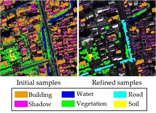
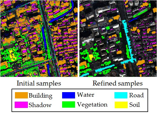
- Select initial training samples of buildings, shadow, water, vegetation, soil, and roads, respectively, from the multiple information sources.
- (2)
- Samples located at the border areas are likely to be mixed pixels, and, thus, it is difficult to automatically assign these pixels to a certain label. In order to avoid introducing incorrect training samples, these border samples are removed with an erosion operation.
- (3)
- Manual sampling always prefers homogeneous areas and disregards outliers. Therefore, in this study, area thresholding is applied to the candidate samples, and the objects whose areas are smaller than a predefined value are removed.
- (4)
- The obtained samples should be further refined, in order to guarantee the accuracy of the samples. Considering the fact that buildings and shadows are always spatially adjacent, the distance between the buildings and their neighboring shadows should be smaller than a threshold, which is used to remove unreliable buildings and shadows from the sample sets. Meanwhile, the road lines obtained from OSM are widened by several pixels, forming a series of buffer areas, where road samples can be picked out.
- (5)
- Considering the difficulty and uncertainty in labelling samples in overlapping regions, the samples that are labeled as more than one class are removed.

| Algorithm: Automatic selection of training samples | |
| 1: | Inputs: |
| 2: | Multiple information sources (MBI, MSI, NDWI, NDVI, HSV, OSM). |
| 3: | Manually selected thresholds (TB, TS, TW, TV). |
| 4: | Step1: Select initial training samples from the information sources. |
| 5: | Step2: Erosion (SE=diamond, radius = 1) is used to remove samples from borders. |
| 6: | Step3: Minimal area (m2): ABuild = 160, AShadow = 20, AWater = 400, AVege = 200, and Asoil = 400. |
| 7: | Step4: Semantic processing: |
| 8: | (1) The distance between buildings and their adjacent shadows is smaller than 10 m (about |
| 9: | five pixels in this study). |
| 10: | (2) Road lines are widened for buffer areas. |
| 11: | Step5: Remove overlapping samples. |
4. Classifiers Considered in This Study
- (1)
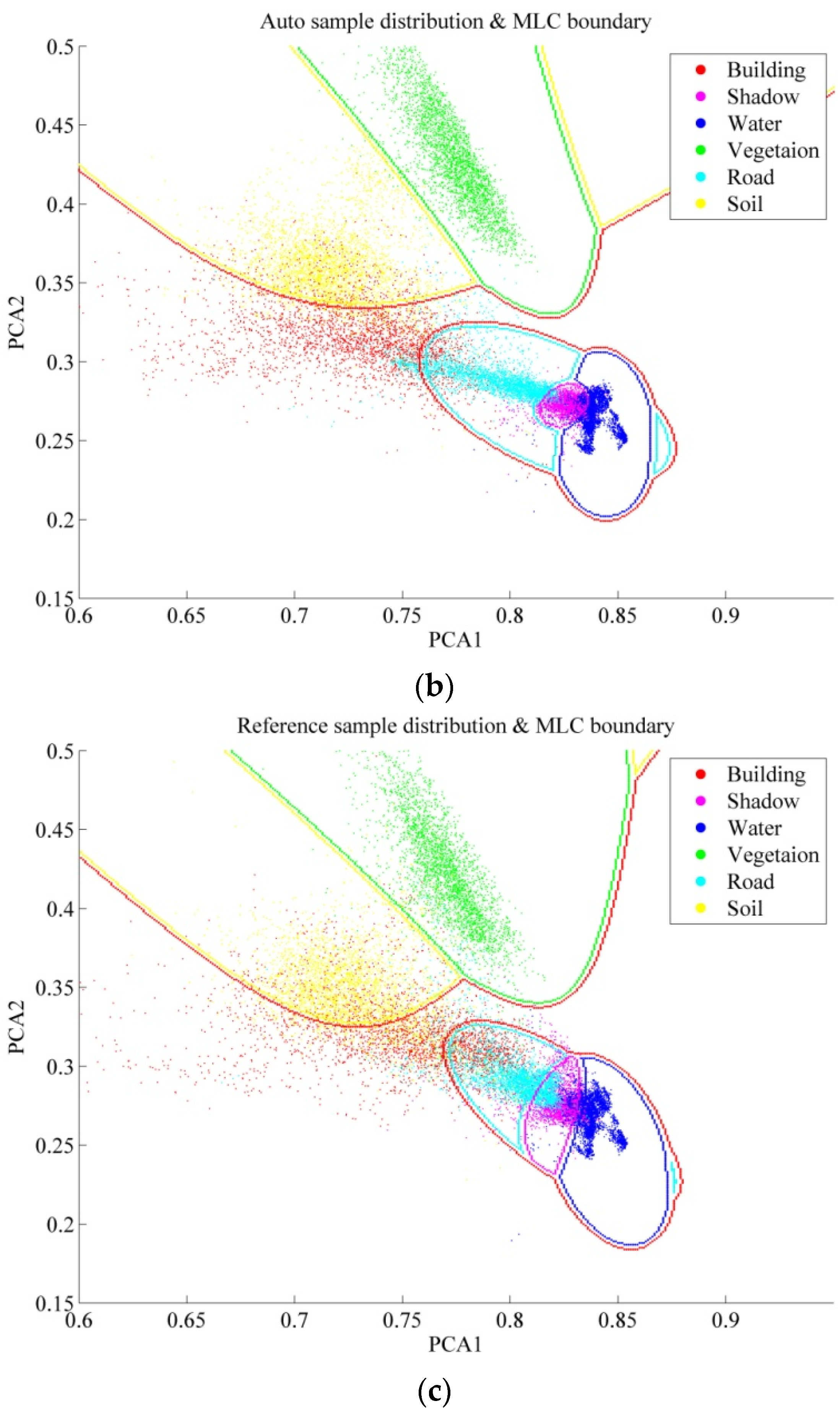
- Maximum Likelihood Classification: MLC is a statistical approach for pattern recognition. For a given pixel, the probability of it belonging to each class is calculated, and it is assigned to the class with the highest probability [14]. Normally, the distribution of each class in the multi-dimension space is assumed to be a Gaussian distribution. The mean and covariance matrix of MLC are obtained from the training samples, and used to effectively model the classes. If the training set is biased compared to the normal distribution, the estimated parameters will not be very accurate.
- (2)
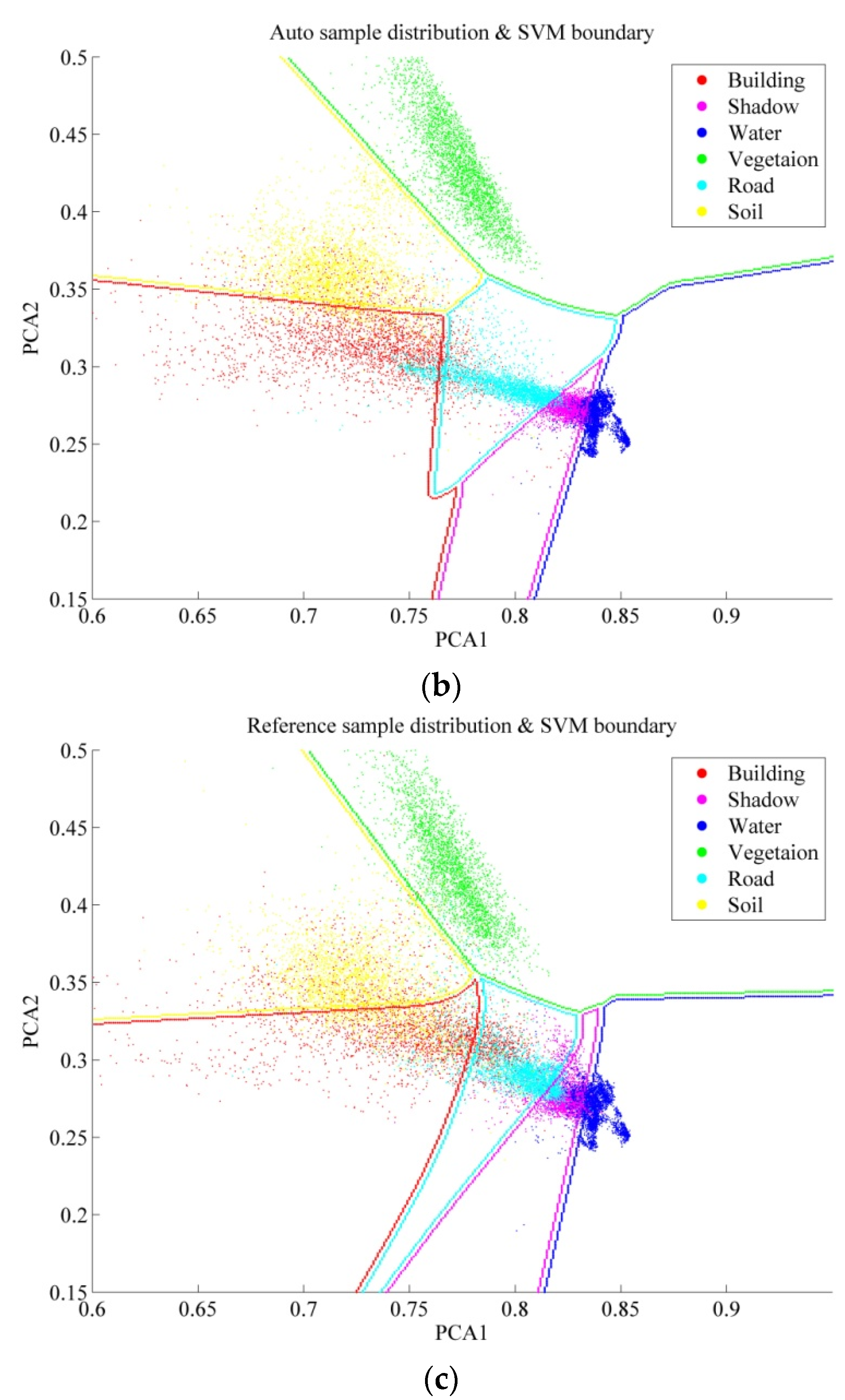
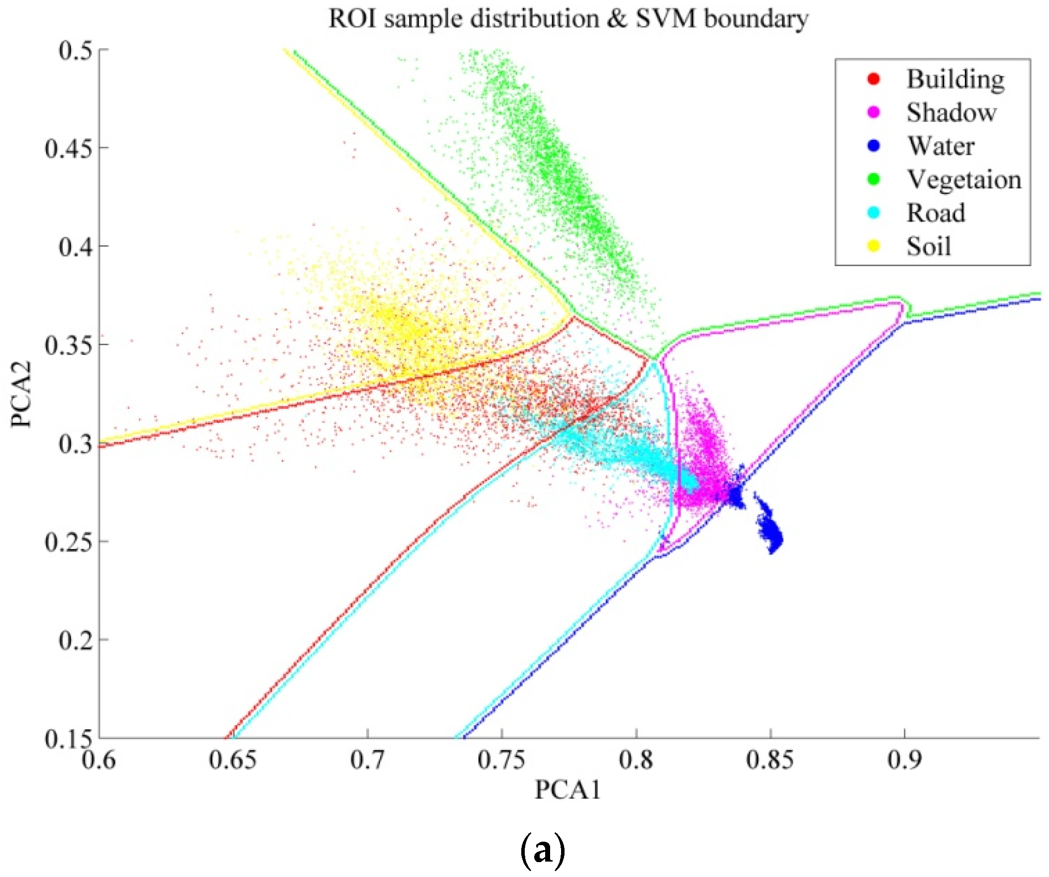
- Support Vector Machine: SVM is a binary classification method based on minimal structural risk, and it can be extended to multi-class classification with multi-class strategies. When dealing with linearly separable datasets, the optimal decision line is obtained by maximizing the margin between the two parallel hyperplanes. This type of SVM ensuring that all the samples are classified correctly is called hard-margin SVM. On the other hand, allowing the existence of misclassified training samples, soft-margin SVM introduces slack variables for each sample. SVM generates nonlinear decision boundaries by mapping the samples from a low-dimension space to a high-dimension one, and the kernel trick is used to avoid the definition of the mapping function [33].An SVM model is constructed by support vectors, which usually locate in the decision boundary region between the class pairs. The most representative and informative samples will be close to the boundary of the class pair [15,34]. A better sample set for training an SVM model is not to accurately describe the classes, but to provide information about the decision boundary between the class pairs in the feature space [35]. Meanwhile, in the case of a small-size sample set, the outliers have an obvious influence on the decision boundary.
- (3)
- Neural Networks: NNs can be viewed as a parallel computing system consisting of an extremely large number of simple processors with interconnections [32]. NNs are able to learn complex nonlinear input-output relationships, use sequential training procedures, and adapt themselves to the data [32]. The MLP is one of the most commonly used NNs. It consists of input, hidden, and output layers, where all the neurons in each layer are fully connected to the neurons in the adjacent layers. These interconnections are associated with numerical weights, which are adjusted iteratively during the training process [36]. Each hidden neuron performs a mapping of the input feature space by a transform function. After an appropriate mapping by the previous layer, the next layer can learn the classification model as a linearly separable problem in the mapped feature space, and thus NNs are able to deal with nonlinearly separable datasets [8]. In this study, the conjugate gradient method (e.g., scaled conjugate gradient, SCG), is used for training of the MLP, since it can avoid the line search at each learning iteration by using a Levenberg-Marquardt approach to scale the step size [36].
- (4)
- Decision Tree: A hierarchical DT classifier is an algorithm for labelling an unknown pattern by the use of a decision sequence. The tree is conducted from the roof node to the terminal leaf, and the feature for each interior node is selected by information gain or the Gini impurity index. A pruning operation is employed in simplifying the DT without increasing errors [14]. Due to the unsatisfactory performance, an ensemble of DTs, such as RF, is more commonly used than the simple DT [37]. RF combines predictors from trees, and the final result of a sample is the most popular class among the trees. Each tree is conducted via a sub-randomly selected sample set and a sub-randomly selected feature space [38]. Each tree in RF is grown to the maximum depth, and not pruned. RF is relatively robust to outliers and noise, and it is insensitive to over-fitting [14].
5. Experiments and Results
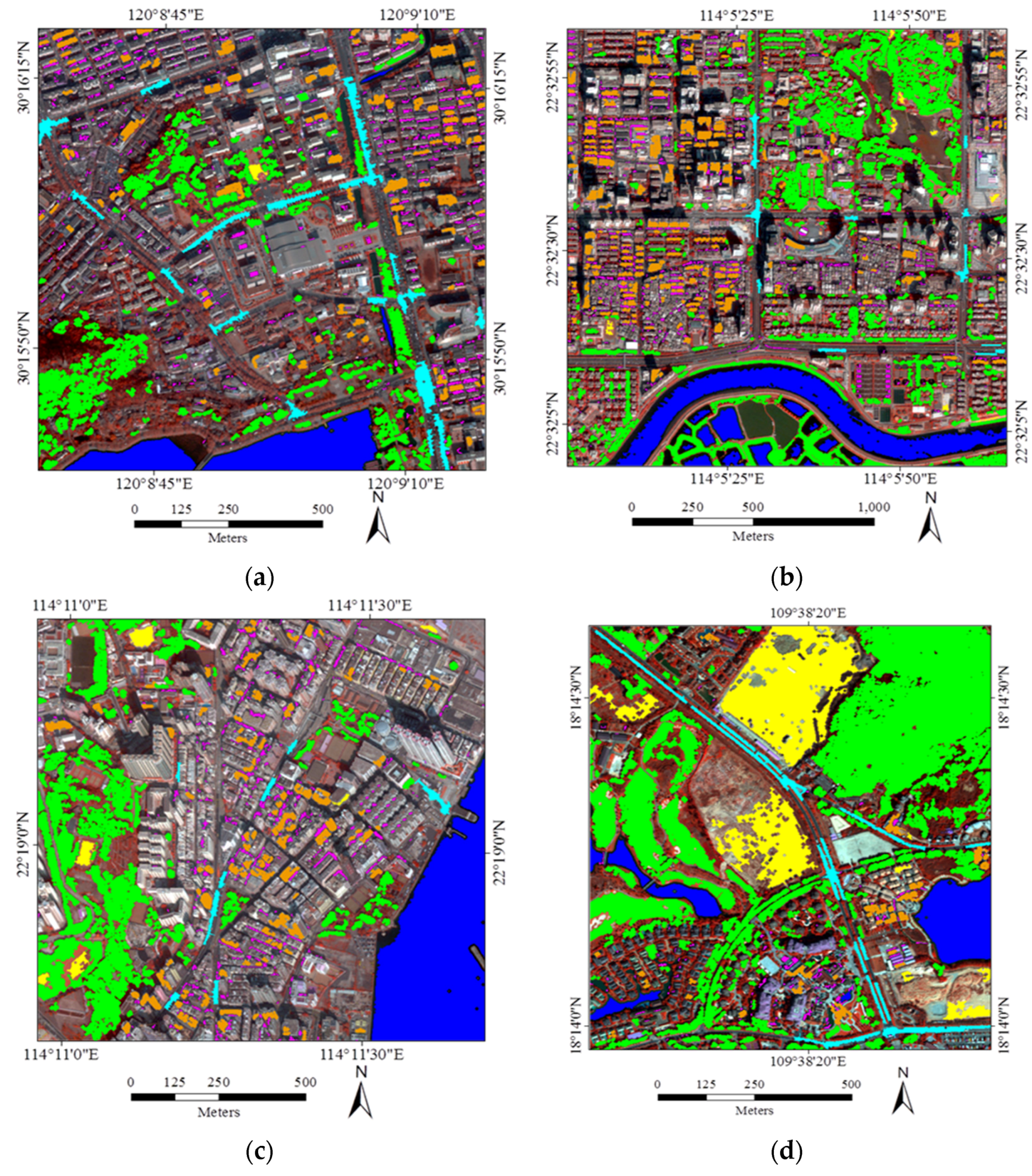
5.1. Datasets and Parameters


| Hangzhou | Shenzhen | Hong Kong | Hainan | |||||
|---|---|---|---|---|---|---|---|---|
| ROI | Test | ROI | Test | ROI | Test | ROI | Test | |
| Building | 13,004 | 19,507 | 16,598 | 24,897 | 12,388 | 18,583 | 4631 | 6947 |
| Shadow | 5742 | 8614 | 9774 | 14,661 | 3788 | 5682 | 570 | 857 |
| Water | 6186 | 9279 | 13,759 | 20,639 | 11,725 | 17,588 | 4,483 | 6726 |
| Vegetation | 7118 | 10,678 | 12,829 | 19,244 | 6042 | 9063 | 8601 | 12,902 |
| Road | 3784 | 5678 | 5185 | 7778 | 1264 | 1898 | 2142 | 3214 |
| Soil | 400 | 601 | 256 | 385 | 496 | 746 | 8875 | 13,314 |
5.2. Results
| Hangzhou | Shenzhen | Hong Kong | Hainan | |
|---|---|---|---|---|
| Buildings | 10,686 | 24,177 | 12,287 | 3208 |
| Shadow | 7282 | 10,306 | 7126 | 1419 |
| Water | 17,418 | 34,307 | 41,569 | 13,572 |
| Vegetation | 29,801 | 83,425 | 44,571 | 85,022 |
| Roads | 8210 | 2938 | 2211 | 6170 |
| Soil | 269 | 852 | 2263 | 27,369 |
| MLC (%) | SVM (%) | RF (%) | MLP (%) | ||
|---|---|---|---|---|---|
| Hangzhou | Auto | 79.3 ± 1.7 | 80.4 ± 2.0 | 82.1 ± 1.2 | 82.6 ± 1.2 |
| ROI | 83.1 ± 1.7 | 85.6 ± 0.8 | 86.8 ± 0.9 | 86.4 ± 1.2 | |
| Shenzhen | Auto | 81.8 ± 0.7 | 84.4 ± 1.0 | 84.0 ± 1.1 | 83.1 ± 2.0 |
| ROI | 82.8 ± 0.9 | 85.0 ± 0.9 | 85.1 ± 0.4 | 85.1 ± 0.8 | |
| Hong Kong | Auto | 91.3 ± 0.6 | 90.2 ± 0.9 | 91.2 ± 0.5 | 91.0 ± 0.7 |
| ROI | 92.2 ± 0.7 | 90.3 ± 1.6 | 90.4 ± 1.1 | 91.1 ± 0.9 | |
| Hainan | Auto | 88.3 ± 0.9 | 86.5 ± 1.9 | 85.4 ± 0.8 | 86.1 ± 0.9 |
| ROI | 94.1 ± 0.5 | 92.4 ± 0.7 | 90.2 ± 0.6 | 93.4 ± 0.5 |
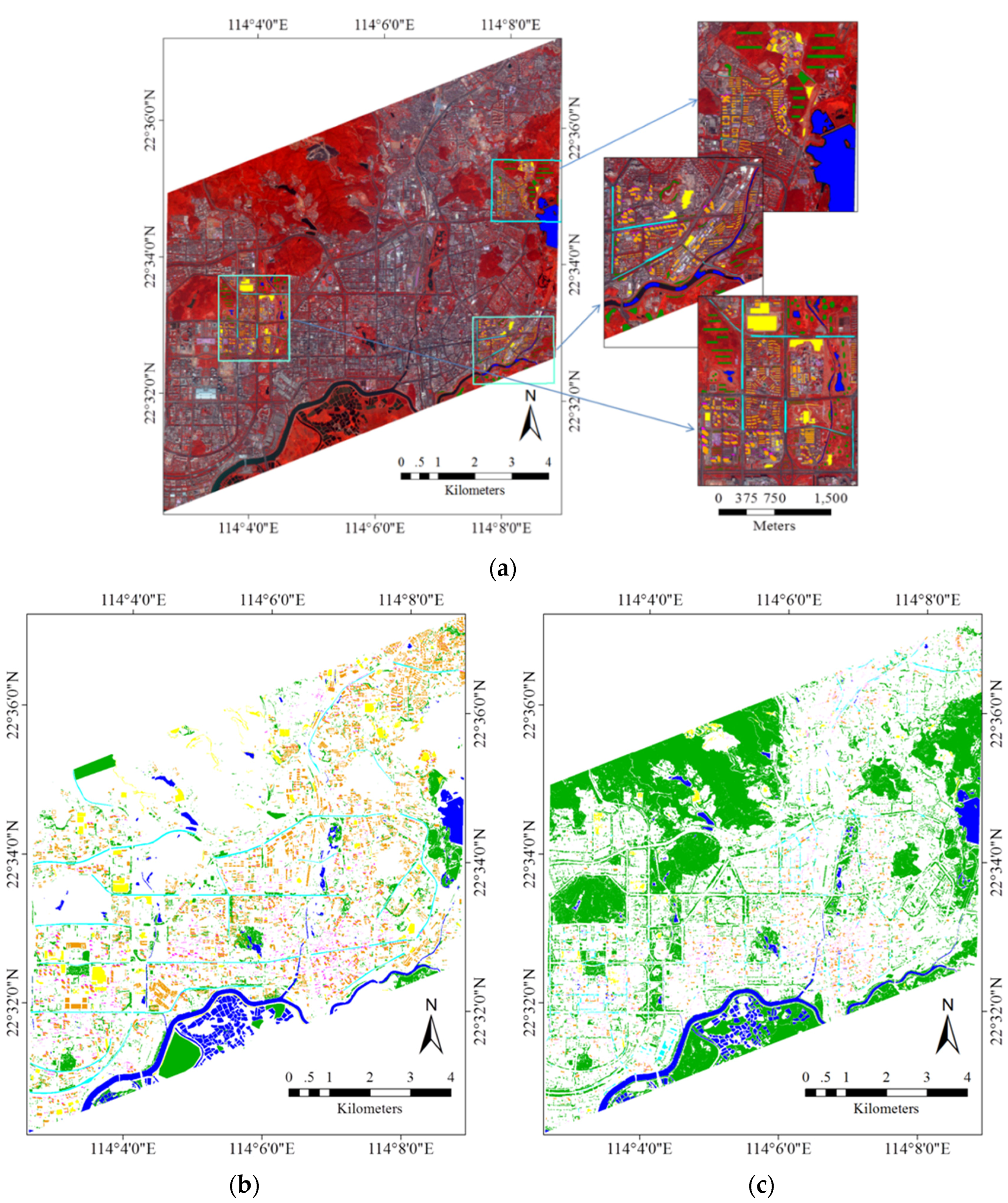
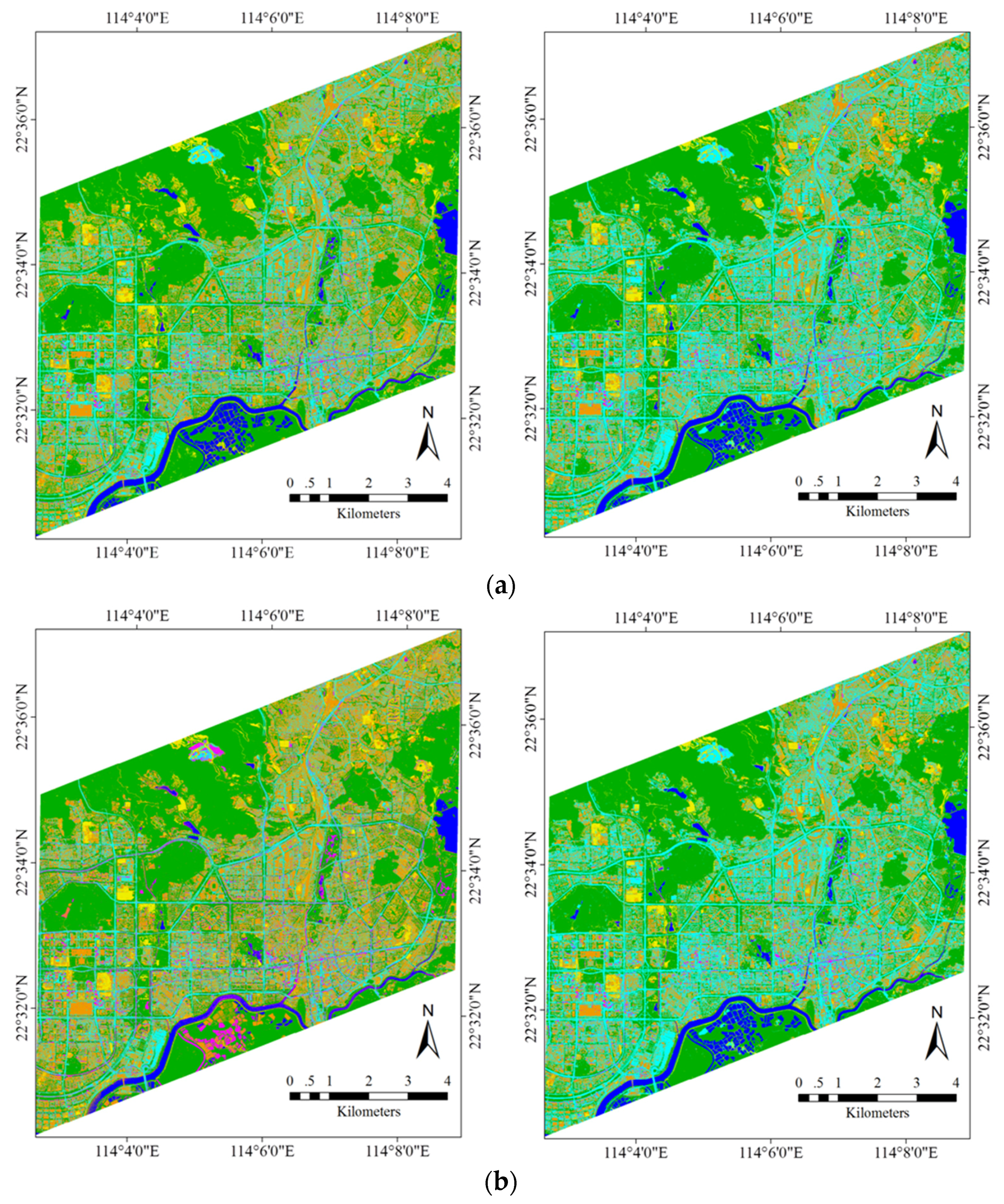
5.3. Large-Size Image Testing
- In general, the classification accuracies obtained by the automatic sampling are very promising (80%~85%), which shows that it is fully possible to automatically classify large-size remote sensing images over urban areas.
- By comparing the performances of the different classifiers, it can be seen that MLC achieves the highest accuracy for the Auto samples, while SVM and the MLP give the best results for the ROI samples.
- It is interesting to see that in the case of MLC, the automatic sampling strategy significantly outperforms the manual sampling by 8% in the overall accuracy.

| Land Cover | ROI | Test | Auto |
|---|---|---|---|
| Buildings | 118,130 | 1,313,843 | 191,811 |
| Shadow | 14,446 | 185,650 | 76,723 |
| Water | 140,823 | 865,113 | 683,317 |
| Vegetation | 98,225 | 1,542,442 | 6,667,588 |
| Roads | 32,942 | 313,572 | 171,312 |
| Soil | 52,944 | 391,949 | 100,707 |
| Strategy | MLC (%) | SVM (%) | RF (%) | MLP (%) |
|---|---|---|---|---|
| Auto | 84.2 ± 1.0 | 81.8 ± 1.7 | 80.9 ± 1.2 | 82.5 ± 0.9 |
| ROI | 76.9 ± 2.2 | 84.0 ± 1.5 | 82.6 ± 1.2 | 84.9 ± 1.3 |
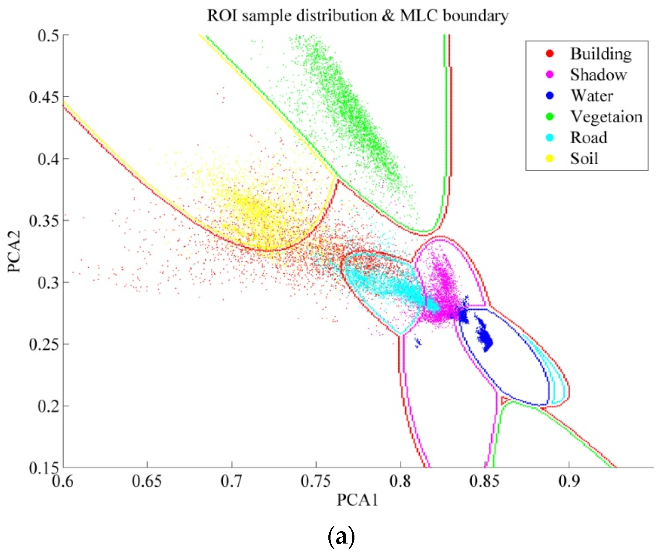
- It should be noted that the Auto samples are purer than ROI, since the automatic selection prefers homogeneous and reliable samples in order to avoid errors and uncertainties. Specifically, as described in Algorithm 1, boundary pixels which are uncertain and mixed have been removed, and the area thresholding further reduces the isolated and heterogeneous pixels.
- The four classifiers considered in this study can be separated into parametric classifiers (MLC), and non-parametric classifiers (SVM, RF, and MLP). The principle of MLC is to construct the distributions for different classes, but the non-parametric methods tend to define the classification decision boundaries between different land-cover classes. Consequently, pure samples are more appropriate for MLC, but an effective sampling for the non-parametric classifiers is highly reliant on the samples near the decision boundaries so that they can be used to separate the different classes.
6. Discussions
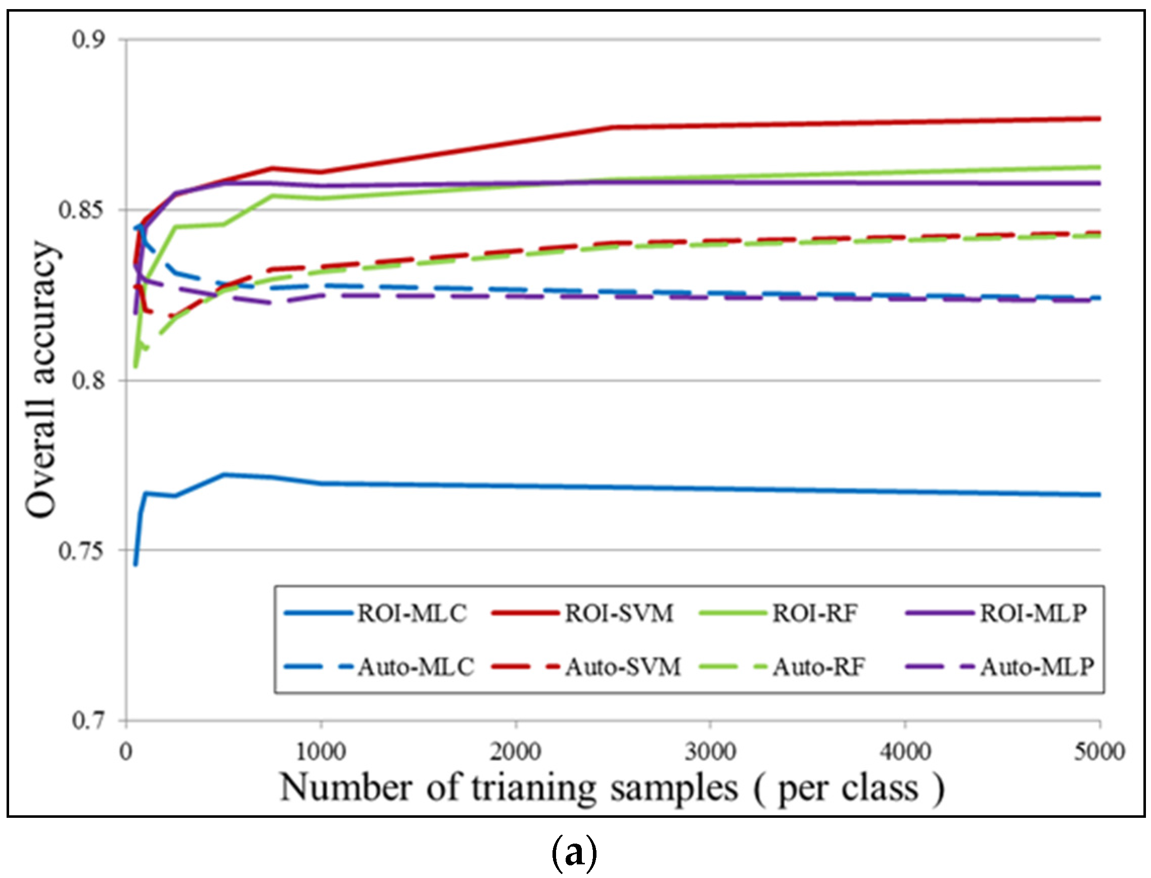
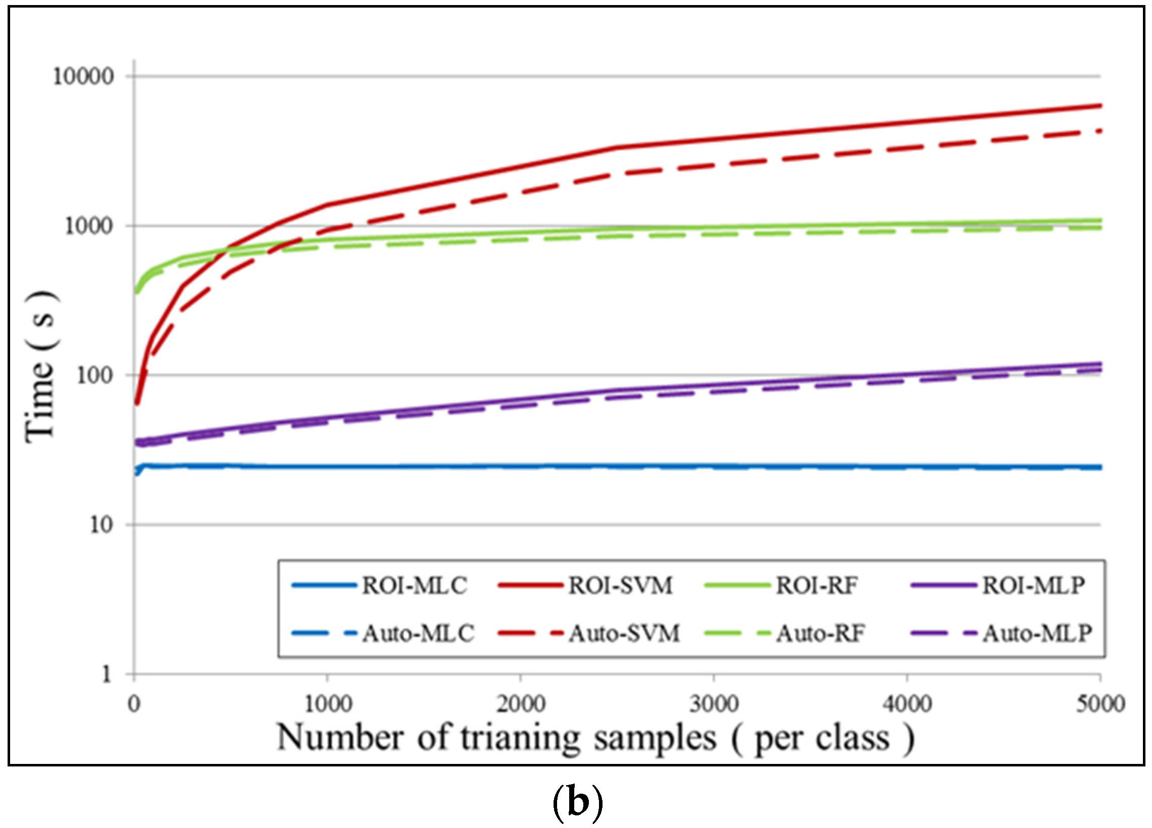
6.1. Number of Training Samples


6.2. Further Comparison Between Auto and ROI Sampling


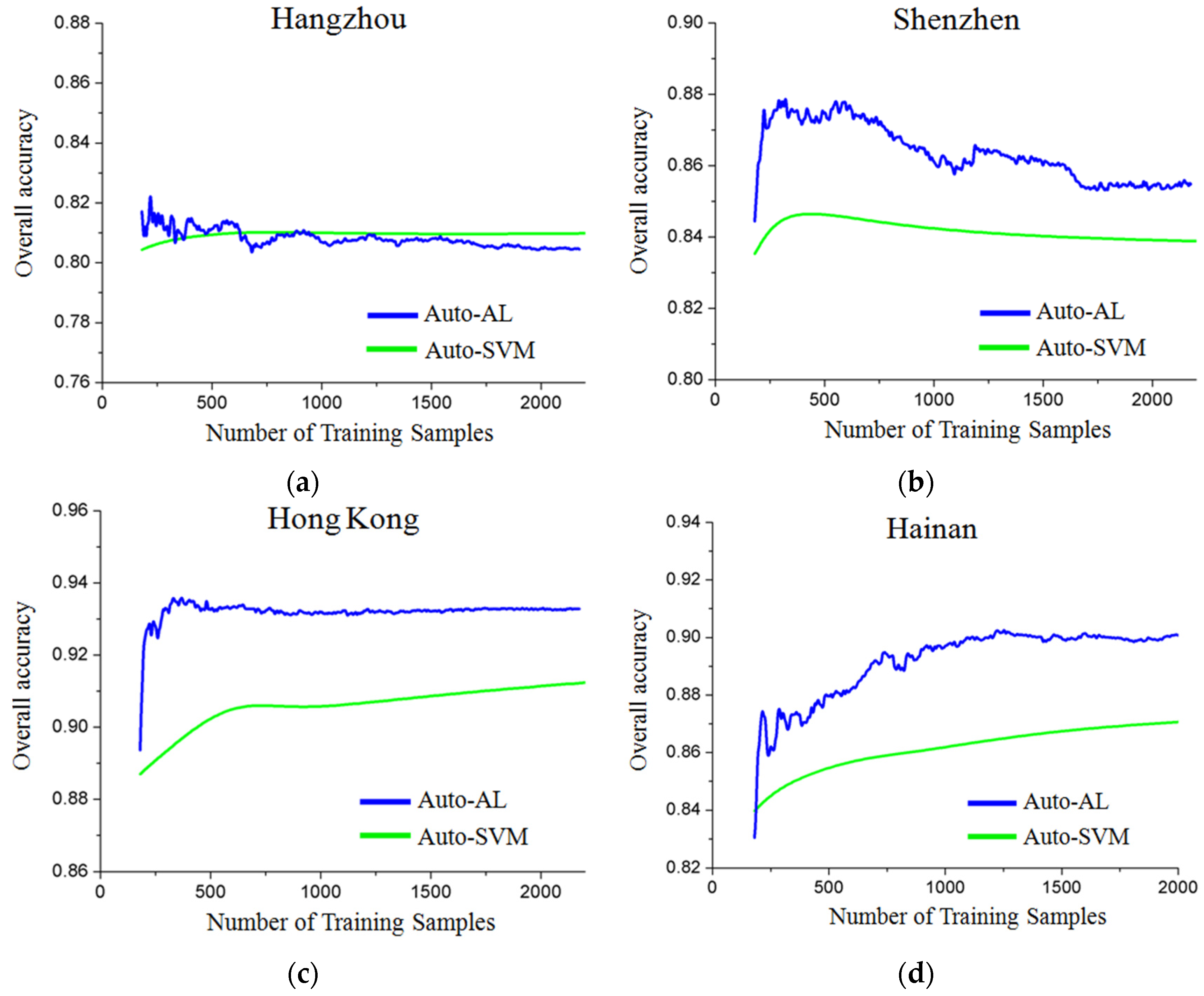
6.3. Active Learning for the Automatic Sampling
7. Conclusions and Future Scope
Acknowledgments
Author Contributions
Conflicts of Interest
References
- Wang, L.; Sousa, W.P.; Gong, P.; Biging, G.S. Comparison of IKONOS and QuickBird images for mapping mangrove species on the caribbean coast of panama. Remote Sens. Environ. 2004, 91, 432–440. [Google Scholar] [CrossRef]
- Zhang, L.; Huang, X.; Huang, B.; Li, P. A pixel shape index coupled with spectral information for classification of high spatial resolution remotely sensed imagery. IEEE Trans. Geosci. Remote Sens. 2006, 44, 2950–2961. [Google Scholar] [CrossRef]
- Dundar, M.M.; Landgrebe, D. A model-based mixture-supervised classification approach in hyperspectral data analysis. IEEE Trans. Geosci. Remote Sens. 2002, 40, 2692–2699. [Google Scholar] [CrossRef]
- Richards, J.A.; Kingsbury, N.G. Is there a preferred classifier for operational thematic mapping? IEEE Trans. Geosci. Remote Sens. 2014, 52, 2715–2725. [Google Scholar] [CrossRef]
- Del Frate, F.; Pacifici, F.; Schiavon, G.; Solimini, C. Use of neural networks for automatic classification from high-resolution images. IEEE Trans. Geosci. Remote Sens. 2007, 45, 800–809. [Google Scholar] [CrossRef]
- Licciardi, G.; Del Frate, F. A neural network approach for pixel unmixing in hyperspectral data. In Proceedings of the 2nd Workshop on Hyperspectral Image and Signal Processing: Evolution in Remote Sensing, Reykjavik, Iceland, 14–16 June 2010.
- Roy, M.; Routaray, D.; Ghosh, S.; Ghosh, A. Ensemble of multilayer perceptrons for change detection in remotely sensed images. IEEE Geosci. Remote Sens. 2014, 11, 49–53. [Google Scholar] [CrossRef]
- Santos, A.B.; de Albuquerque Araújo, A.; Menotti, D. Combining multiple classification methods for hyperspectral data interpretation. IEEE J. Sel. Top. Appl. Earth Observ. Remote Sens. 2013, 6, 1450–1459. [Google Scholar] [CrossRef]
- Melgani, F.; Bruzzone, L. Classification of hyperspectral remote sensing images with support vector machines. IEEE Trans. Geosci. Remote Sens. 2004, 42, 1778–1790. [Google Scholar] [CrossRef]
- Bruzzone, L.; Carlin, L. A multilevel context-based system for classification of very high spatial resolution images. IEEE Trans. Geosci. Remote Sens. 2006, 44, 2587–2600. [Google Scholar] [CrossRef]
- Huang, X.; Zhang, L. An SVM ensemble approach combining spectral, structural, and semantic features for the classification of high-resolution remotely sensed imagery. IEEE Trans. Geosci. Remote Sens. 2013, 51, 257–272. [Google Scholar] [CrossRef]
- Huang, X.; Zhang, L. Comparison of vector stacking, multi-SVMs fuzzy output, and multi-svms voting methods for multiscale vhr urban mapping. IEEE Geosci. Remote Sens. Lett. 2010, 7, 261–265. [Google Scholar] [CrossRef]
- Pal, M.; Foody, G.M. Feature selection for classification of hyperspectral data by SVM. IEEE Trans. Geosci. Remote Sens. 2010, 48, 2297–2307. [Google Scholar] [CrossRef]
- Mather, P.; Tso, B. Classification Methods for Remotely Sensed Data, 2nd ed.; Taylor and Francis: Abingdon, UK, 2004. [Google Scholar]
- Tuia, D.; Volpi, M.; Copa, L.; Kanevski, M.; Munoz-Mari, J. A survey of active learning algorithms for supervised remote sensing image classification. IEEE J. Sel. Top. Signal Process. 2011, 5, 606–617. [Google Scholar] [CrossRef]
- Demir, B.; Persello, C.; Bruzzone, L. Batch-mode active-learning methods for the interactive classification of remote sensing images. IEEE Trans. Geosci. Remote Sens. 2011, 49, 1014–1031. [Google Scholar] [CrossRef]
- Di, W.; Crawford, M.M. View generation for multiview maximum disagreement based active learning for hyperspectral image classification. IEEE Trans. Geosci. Remote Sens. 2012, 50, 1942–1954. [Google Scholar] [CrossRef]
- Patra, S.; Bruzzone, L. A novel SOM-SVM-Based active learning technique for remote sensing image classification. IEEE Trans. Geosci. Remote Sens. 2014, 52, 6899–6910. [Google Scholar] [CrossRef]
- Persello, C.; Boularias, A.; Dalponte, M.; Gobakken, T.; Naesset, E.; Scholkopf, B. Cost-sensitive active learning with lookahead: Optimizing field surveys for remote sensing data classification. IEEE Trans. Geosci. Remote Sens. 2014, 52, 6652–6664. [Google Scholar] [CrossRef]
- Mitra, P.; Shankar, B.U.; Pal, S.K. Segmentation of multispectral remote sensing images using active support vector machines. Pattern Recognit. Lett. 2004, 25, 1067–1074. [Google Scholar] [CrossRef]
- Persello, C.; Bruzzone, L. Active learning for domain adaptation in the supervised classification of remote sensing images. IEEE Trans. Geosci. Remote Sens. 2012, 50, 4468–4483. [Google Scholar] [CrossRef]
- Rajan, S.; Ghosh, J.; Crawford, M.M. An active learning approach to hyperspectral data classification. IEEE Trans. Geosci. Remote Sens. 2008, 46, 1231–1242. [Google Scholar] [CrossRef]
- Sinno Jialin, P.; Qiang, Y. A survey on transfer learning. IEEE Trans. Knowl. Data Eng. 2010, 22, 1345–1359. [Google Scholar]
- Huang, X.; Zhang, L. A multidirectional and multiscale morphological index for automatic building extraction from multispectral GeoEye-1 imagery. Photogramm. Eng. Remote Sens. 2011, 77, 721–732. [Google Scholar] [CrossRef]
- Huang, X.; Zhang, L. Morphological building/shadow index for building extraction from high-resolution imagery over urban areas. IEEE J. Sel. Top. Appl. Earth Observ. Remote Sens. 2012, 5, 161–172. [Google Scholar] [CrossRef]
- Gao, B.-C. NDWI—A normalized difference water index for remote sensing of vegetation liquid water from space. Remote Sens. Environ. 1996, 58, 257–266. [Google Scholar] [CrossRef]
- Goward, S.N.; Markham, B.; Dye, D.G.; Dulaney, W.; Yang, J. Normalized difference vegetation index measurements from the advanced very high resolution radiometer. Remote Sens. Environ. 1991, 35, 257–277. [Google Scholar] [CrossRef]
- Bennett, J. Openstreetmap: Be Your Own Cartographer; Packt Publishing: Birmingham, UK, 2010. [Google Scholar]
- Huang, X.; Lu, Q.; Zhang, L. A multi-index learning approach for classification of high-resolution remotely sensed images over urban areas. ISPRS J. Photogramm. Remote Sens. 2014, 90, 36–48. [Google Scholar] [CrossRef]
- Tang, Y.; Huang, X.; Zhang, L. Fault-tolerant building change detection from urban high-resolution remote sensing imagery. IEEE Geosci. Remote Sens Lett. 2013, 10, 1060–1064. [Google Scholar] [CrossRef]
- Wikipedia. Available online: https://en.wikipedia.org/wiki/HSL_and_HSV (accessed on 25 November 2015).
- Jain, A.K.; Duin, R.P.W.; Mao, J. Statistical pattern recognition: A review. IEEE Trans. Pattern Anal Mach. Intell. 2000, 22, 4–37. [Google Scholar] [CrossRef]
- Abe, S. Support Vector Machines for Pattern Classification; Springer: Berlin, Germany, 2010. [Google Scholar]
- Zadrozny, B. Learning and evaluating classifiers under sample selection bias. In Proceedings of the 21th International Conference on Machine Learning, Banff, AB, Canada, 4–8 June 2004.
- Foody, G.M.; Mathur, A. The use of small training sets containing mixed pixels for accurate hard image classification: Training on mixed spectral responses for classification by a svm. Remote Sens. Environ. 2006, 103, 179–189. [Google Scholar] [CrossRef]
- Møller, M.F. A scaled conjugate gradient algorithm for fast supervised learning. Neural Netw. 1993, 6, 525–533. [Google Scholar] [CrossRef]
- Breiman, L. Random forests. Mach. Learn. 2001, 45, 5–32. [Google Scholar] [CrossRef]
- Pal, M. Random forest classifier for remote sensing classification. Int. J. Remote Sens. 2005, 26, 217–222. [Google Scholar] [CrossRef]
- Luo, T.; Kramer, K.; Samson, S.; Remsen, A.; Goldgof, D.B.; Hall, L.O.; Hopkins, T. In Active learning to recognize multiple types of plankton. In Proceedings of the 17th International Conference on Pattern Recognition, Cambridge, UK, 23–26 August 2004; Volume 473, pp. 478–481.
- Persello, C.; Bruzzone, L. Active and semisupervised learning for the classification of remote sensing images. IEEE Trans. Geosci. Remote Sens. 2014, 52, 6937–6956. [Google Scholar] [CrossRef]
- Olofsson, P.; Foody, G.M.; Herold, M.; Stehman, S.V.; Woodcock, C.E.; Wulder, M.A. Good practices for estimating area and assessing accuracy of land change. Remote Sens. Environ. 2014, 148, 42–57. [Google Scholar] [CrossRef]
© 2015 by the authors; licensee MDPI, Basel, Switzerland. This article is an open access article distributed under the terms and conditions of the Creative Commons by Attribution (CC-BY) license (http://creativecommons.org/licenses/by/4.0/).
Share and Cite
Huang, X.; Weng, C.; Lu, Q.; Feng, T.; Zhang, L. Automatic Labelling and Selection of Training Samples for High-Resolution Remote Sensing Image Classification over Urban Areas. Remote Sens. 2015, 7, 16024-16044. https://doi.org/10.3390/rs71215819
Huang X, Weng C, Lu Q, Feng T, Zhang L. Automatic Labelling and Selection of Training Samples for High-Resolution Remote Sensing Image Classification over Urban Areas. Remote Sensing. 2015; 7(12):16024-16044. https://doi.org/10.3390/rs71215819
Chicago/Turabian StyleHuang, Xin, Chunlei Weng, Qikai Lu, Tiantian Feng, and Liangpei Zhang. 2015. "Automatic Labelling and Selection of Training Samples for High-Resolution Remote Sensing Image Classification over Urban Areas" Remote Sensing 7, no. 12: 16024-16044. https://doi.org/10.3390/rs71215819
APA StyleHuang, X., Weng, C., Lu, Q., Feng, T., & Zhang, L. (2015). Automatic Labelling and Selection of Training Samples for High-Resolution Remote Sensing Image Classification over Urban Areas. Remote Sensing, 7(12), 16024-16044. https://doi.org/10.3390/rs71215819