
A Wavelet-Based Area Parameter for Indirectly Estimating Copper Concentration in Carex Leaves from Canopy Reflectance


Abstract
:
1. Introduction
2. Materials
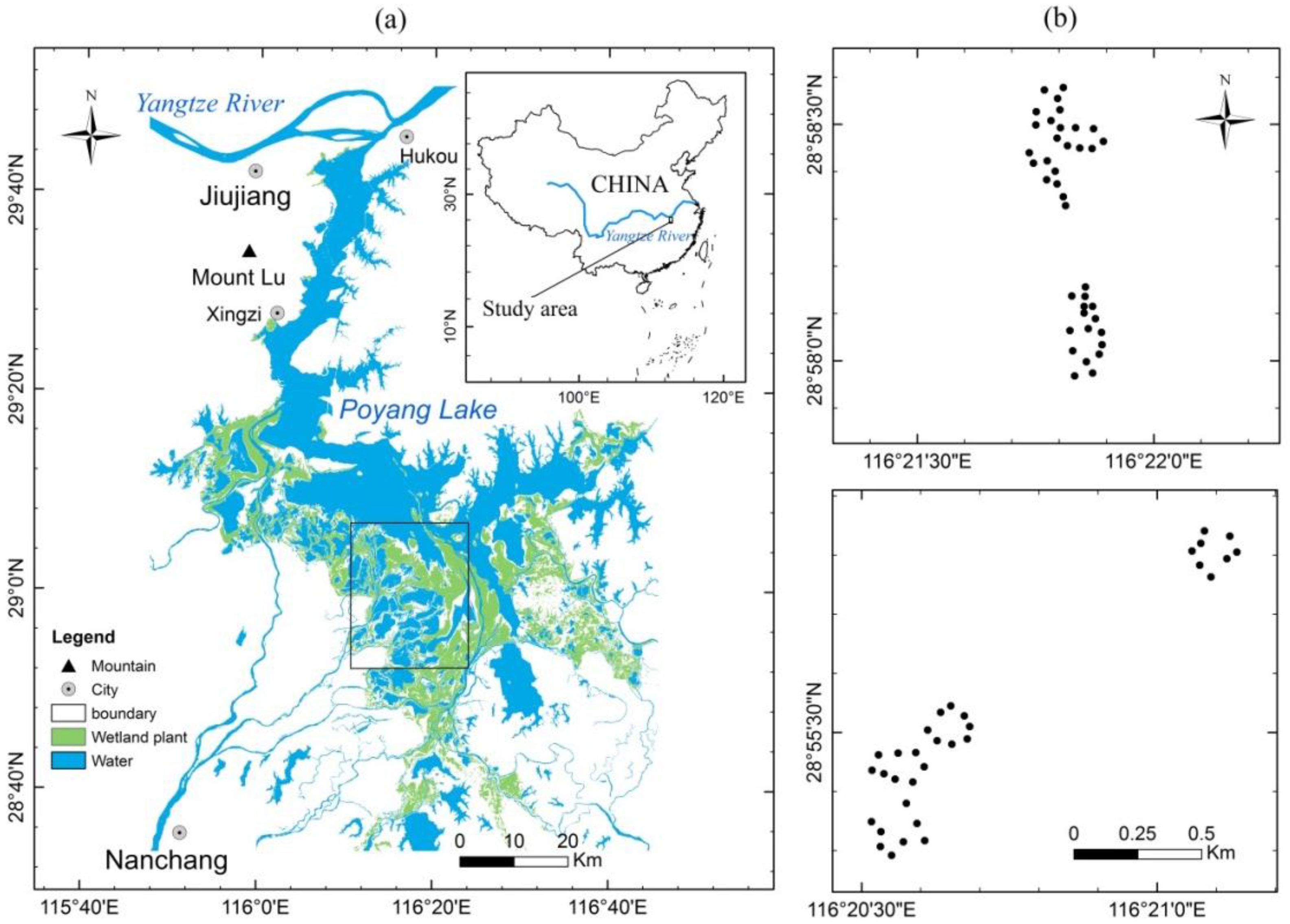
2.1. Study Area

2.2. Data Collection
2.3. Spectral Pre-Processing
3. Methods
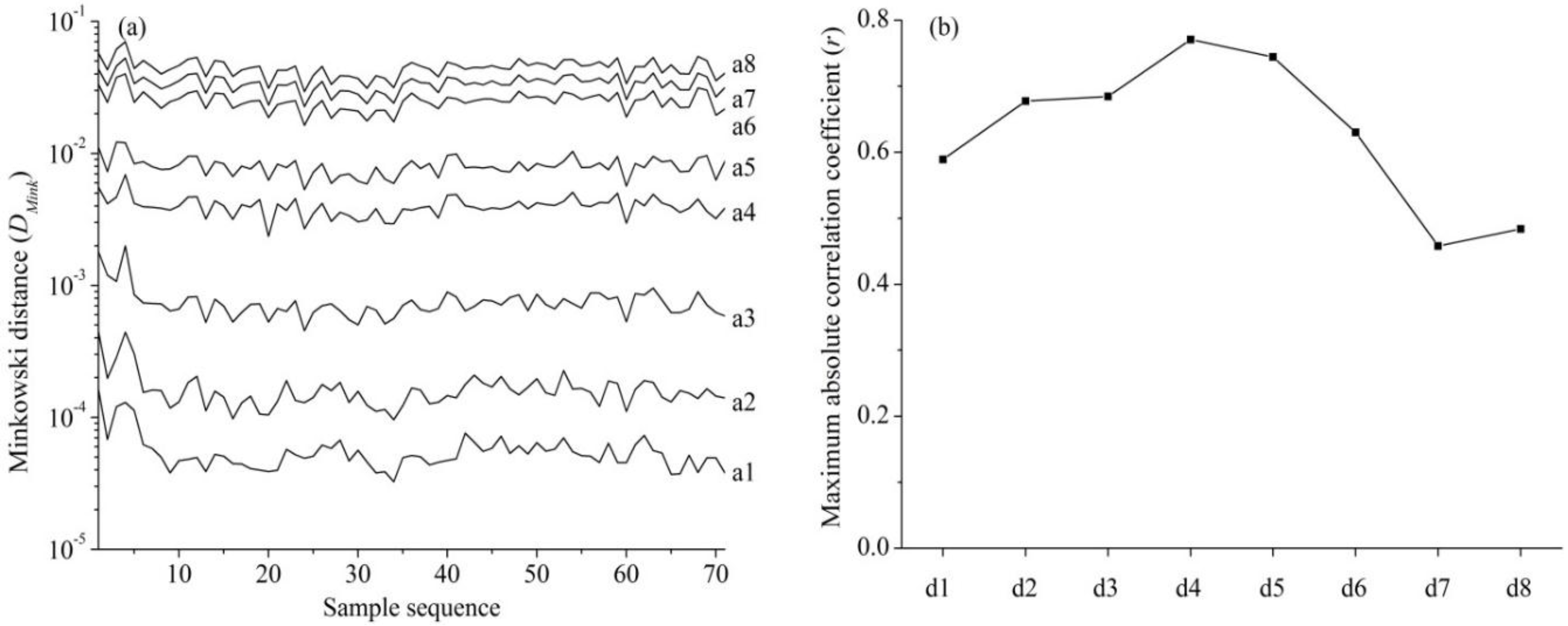
3.1. Selection of Mother Wavelet Function for Wavelet Transform
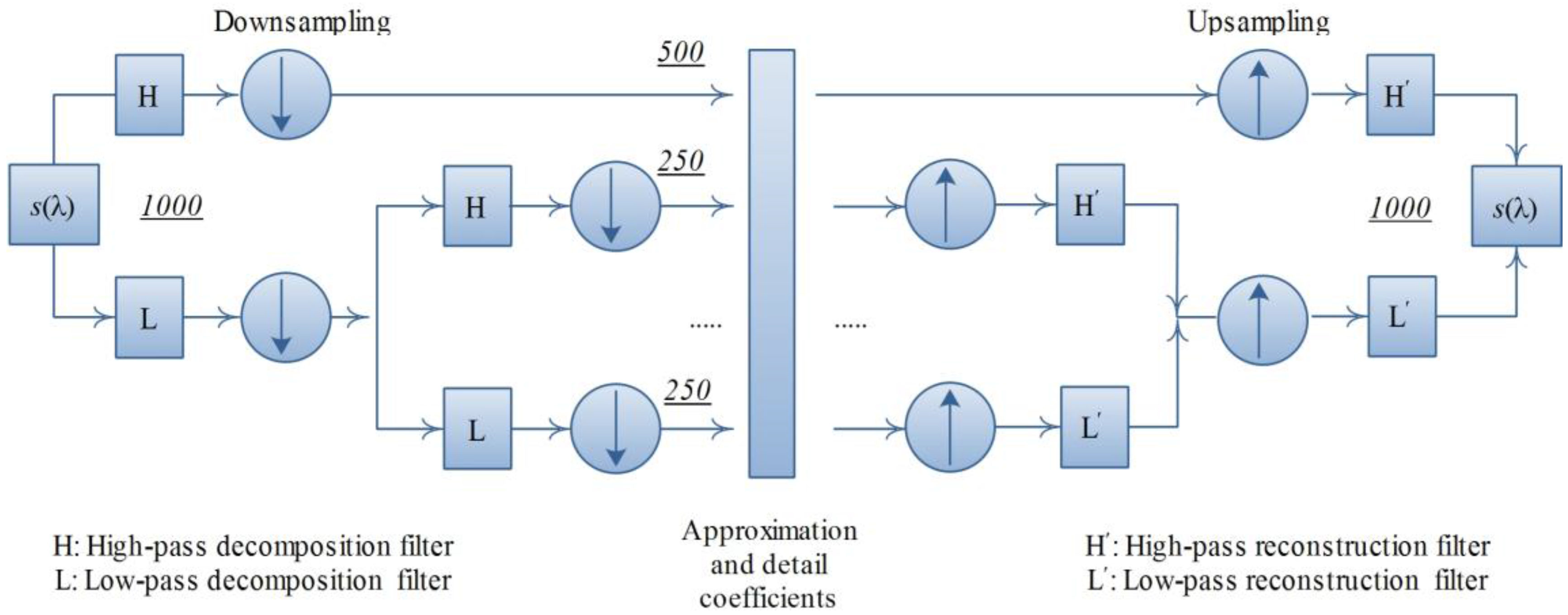
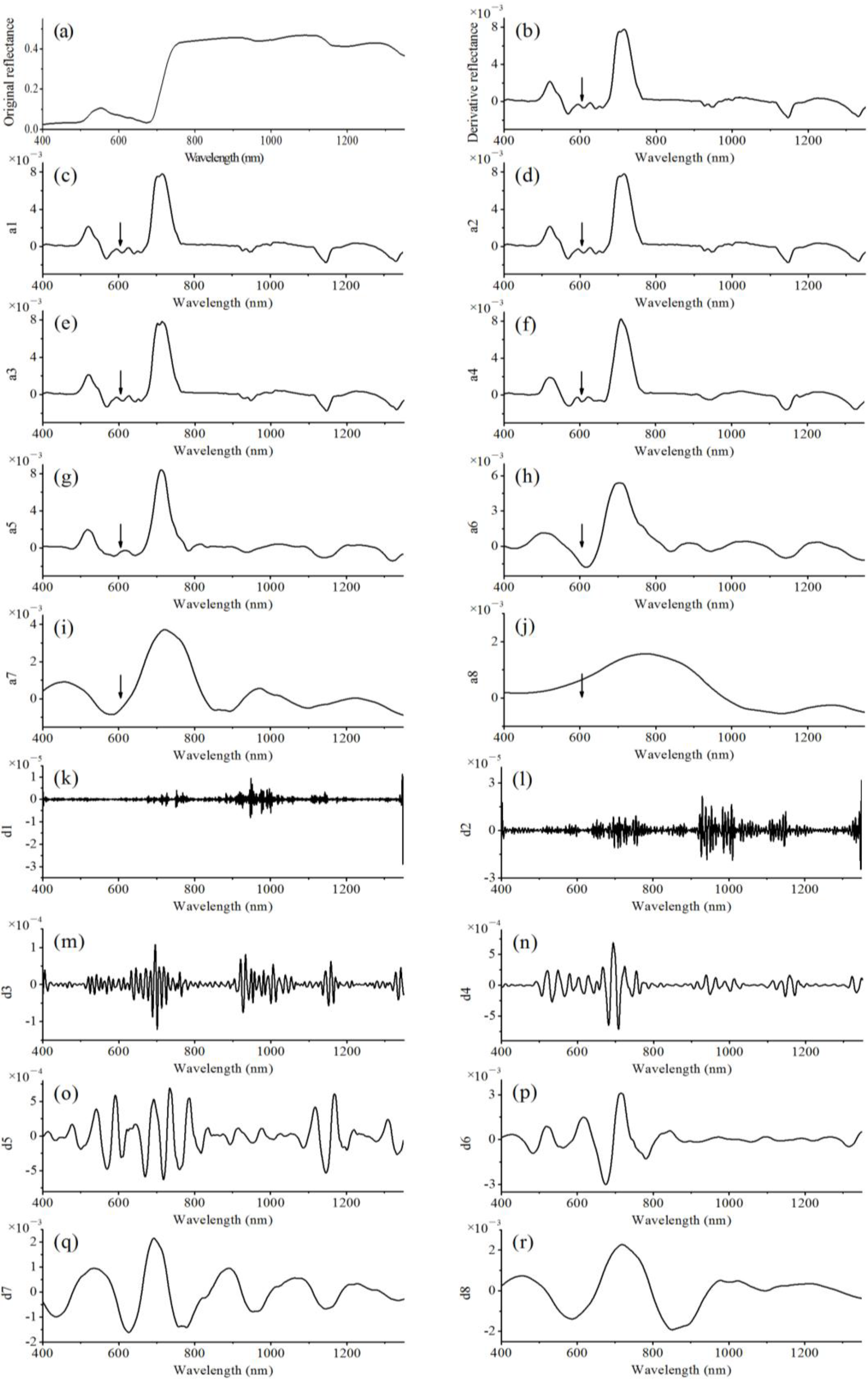
3.2. Spectral Decomposition and Reconstruction Using Discrete Wavelet Transform
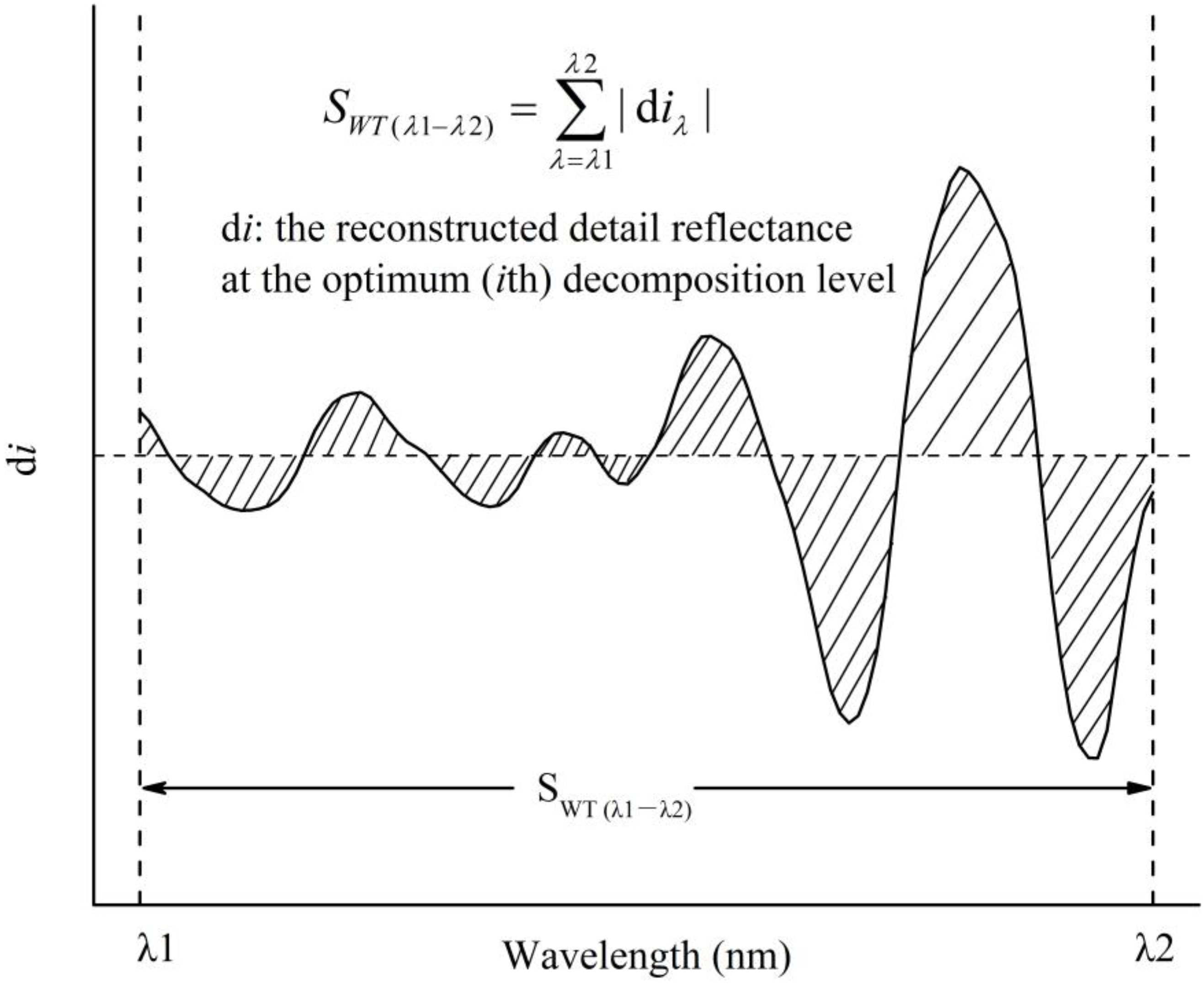
3.3. Defining a Wavelet-Based Area Parameter Using Discrete Wavelet Transform
- Selection of the optimal decomposition level for DWT analysis of pre-processed reflectance (i.e., first derivative reflectance);
- Rough identification of the spectral region (λ1 − λ2 nm) sensitive to foliar Cu variations;
- Optimization of the spectral region for the area parameter.
- (1)
- The reconstructed approximation reflectance was required to maximize the spectral similarity of first derivative reflectance to ensure the general shape and localization of spectral features;
- (2)
- The reconstructed detail reflectance required maximizing the correlation with foliar Cu concentrations to magnify the subtle spectral information.

3.4. Estimation of Foliar Cu Concentration Using the Wavelet-Based Area Parameter
3.5. Performance Comparison between the Wavelet-Based Area Parameter and Published Spectral Parameters

| Spectral Parameter | Formula | Reference |
|---|---|---|
| Modified simple ratio (MSR [670, 800]) | Chen [17] | |
| Modified simple ratio (MSR [500, 720]) | Le Maire et al. [13] | |
| Normalized difference (ND [710, 925] | Le Maire et al. [19] | |
| Modified normalized difference (MND [445, 750]) | Sims and Gamon [16] | |
| Modified Chlorophyll absorption ratio index (MCARI [670, 700]) | Daughtry et al. [11] | |
| Optimized soil-adjusted vegetation index (OSAVI [670, 800]) | Rondeaux et al. [47] | |
| MCARI/OSAVI [705, 750] | Wu et al. [14] | |
| Red edge position (REP) | Cho and Skidmore [20] | |
| Red edge area (SRE) | Filella et al. [30] | |
| Normalized area over reflectance curve (NAOC [643, 795]) | Delegido et al. [18] |
4. Results
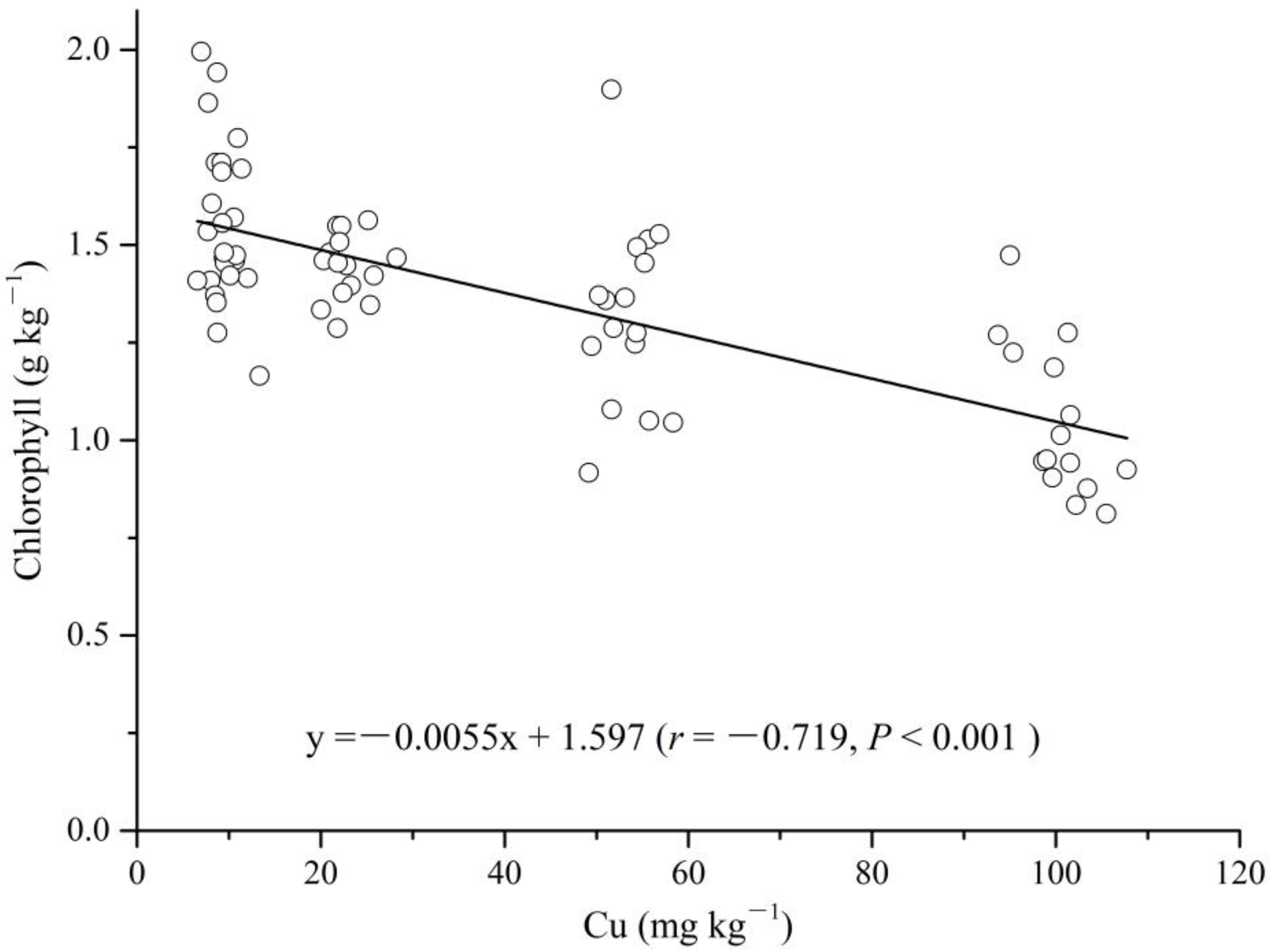
4.1. Relationship between Foliar Cu and Chlorophyll Concentration

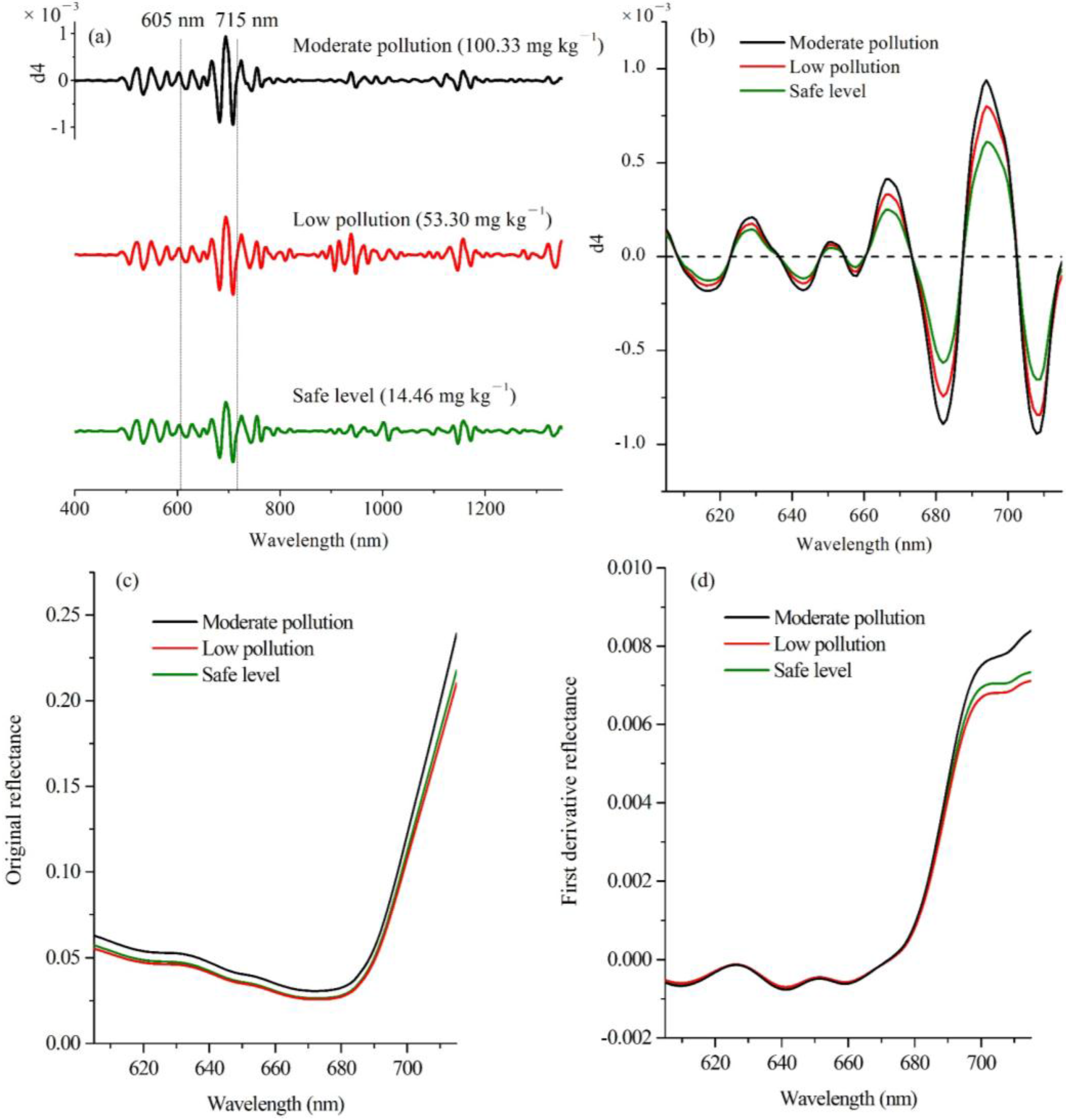
4.2. Extraction of the Wavelet-Based Area Parameter from Canopy Reflectance Spectra

| λ1 (nm) | λ2 (nm) | r | λ1 (nm) | λ2 (nm) | r |
|---|---|---|---|---|---|
| 605 | 715 | 0.836 | 605 | 715 | 0.836 |
| 720 | 0.838 | 600 | 0.832 | ||
| 725 | 0.835 | 595 | 0.816 | ||
| 730 | 0.832 | 590 | 0.805 | ||
| 735 | 0.831 | 585 | 0.794 | ||
| 740 | 0.827 | 580 | 0.782 | ||
| 745 | 0.815 | 575 | 0.779 | ||
| 750 | 0.807 | 570 | 0.758 | ||
| 755 | 0.791 | 565 | 0.723 | ||
| 760 | 0.778 | 560 | 0.720 | ||
| 765 | 0.762 | 555 | 0.718 |

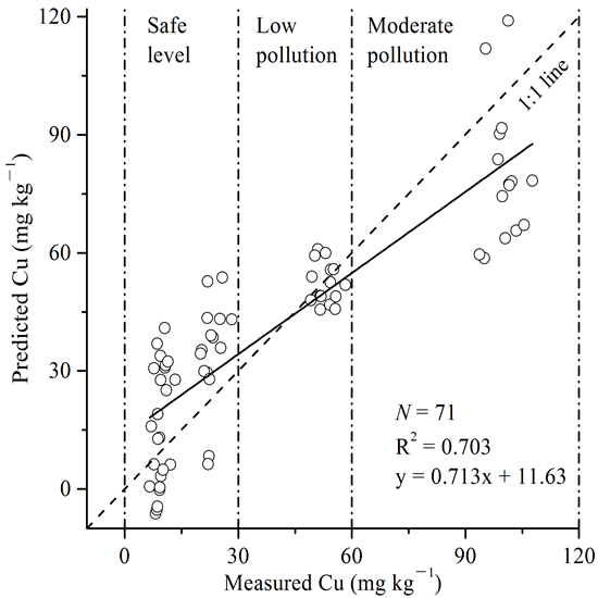
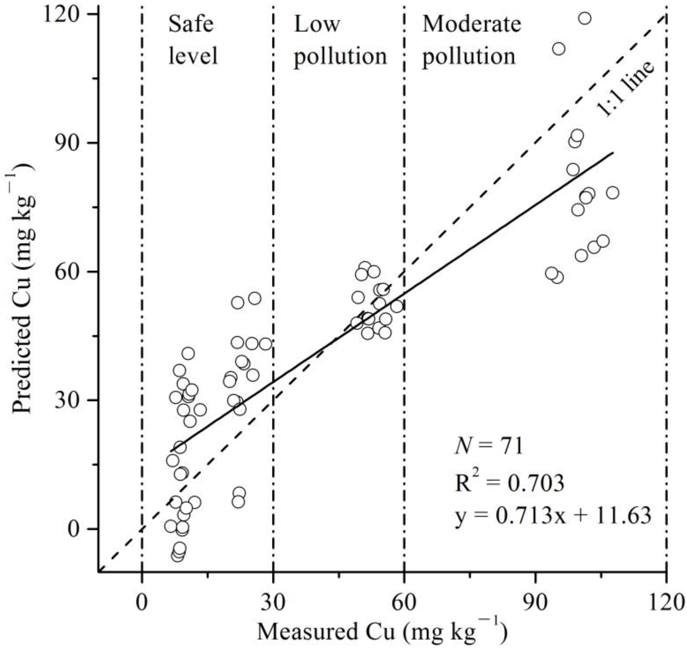
4.3. Foliar Cu Estimation with the Wavelet-Based Area Parameter
| Statistics | Calibration (N = 36) | Validation (N = 35) | |||||
|---|---|---|---|---|---|---|---|
| k | b | RMSECal (mg∙kg−1) | R2Cal | RMSEVal (mg∙kg−1) | R2Val | RPD | |
| Minimum | 5176.71 | -193.28 | 11.82 | 0.491** | 14.49 | 0.516** | 1.16 |
| Maximum | 9800.62 | -89.55 | 22.67 | 0.885** | 26.91 | 0.822** | 2.24 |
| Mean | 7098.05 | -129.12 | 18.37 | 0.710** | 20.16 | 0.706** | 1.75 |
4.4. Performance Comparison between the Wavelet-Based Area Parameter and Published Spectral Parameters
| Spectral Parameter | Mean | LCL 95% | UCL 95% |
|---|---|---|---|
| MSR [670, 800] | 0.087 | 0.001 | 0.218 |
| MSR [500, 720] | 0.192** | 0.040 | 0.315 |
| ND [710, 925] | 0.193** | 0.058 | 0.336 |
| MND [445, 750] | 0.187** | 0.055 | 0.312 |
| MCARI [670, 700] | 0.515** | 0.394 | 0.614 |
| OSAVI [670, 800] | 0.168** | 0.021 | 0.327 |
| MCARI/OSAVI [705, 750] | 0.039 | 0.010 | 0.157 |
| REP | 0.178** | 0.038 | 0.305 |
| SRE | 0.214** | 0.046 | 0.393 |
| NAOC [643, 795] | 0.136* | 0.027 | 0.262 |
| FDWT480−850 | 0.145* | 0.107 | 0.276 |
| SWT (605−720) (this paper) | 0.706** | 0.570 | 0.773 |
5. Discussion
6. Conclusions
- (1)
- The wavelet-based area parameter could be used to indirectly estimate foliar Cu concentration through the strong correlation between Cu and chlorophyll;
- (2)
- The wavelet-based area parameter has the potential ability of detecting low concentrations of Cu pollution in Carex leaves;
- (3)
- The wavelet-based area parameter was superior to published chlorophyll-related and wavelet-based spectral parameters for estimating Cu concentration in Carex leaves.
Acknowledgments
Author Contributions
Conflicts of Interest
References
- Hall, J. Cellular mechanisms for heavy metal detoxification and tolerance. J. Exp. Bot. 2002, 53, 1–11. [Google Scholar] [CrossRef] [PubMed]
- Dietz, K.J.; Baier, M.; Krämer, U. Free radicals and reactive oxygen species as mediators of heavy metal toxicity in plants. In Heavy Metal Stress in Plants; Prasad, M.N.V., Hagemeyer, J., Eds.; Springer: Berlin, Germany, 1999; pp. 73–97. [Google Scholar]
- Krause, G.H.; Kaiser, H. Plant response to heavy metals and sulphur dioxide. Environ. Pollut. 1977, 12, 63–71. [Google Scholar] [CrossRef]
- Macinnis-Ng, C.M.; Ralph, P.J. Towards a more ecologically relevant assessment of the impact of heavy metals on the photosynthesis of the seagrass, Zostera capricorni. Mar. Pollut. Bull. 2002, 45, 100–106. [Google Scholar] [CrossRef]
- Markert, B. Plants as Biomonitors: Indicators for Heavy Metals in the Terrestrial Environment; VCH Publishers Ltd.: Cambridge, UK, 1993. [Google Scholar]
- Kooistra, L.; Salas, E.; Clevers, J.; Wehrens, R.; Leuven, R.; Nienhuis, P.; Buydens, L. Exploring field vegetation reflectance as an indicator of soil contamination in river floodplains. Environ. Pollut. 2004, 127, 281–290. [Google Scholar] [CrossRef]
- Schlerf, M.; Atzberger, C.; Hill, J. Remote sensing of forest biophysical variables using HyMap imaging spectrometer data. Remote Sens. Environ. 2005, 95, 177–194. [Google Scholar] [CrossRef]
- Curran, P.J.; Dungan, J.L.; Peterson, D.L. Estimating the foliar biochemical concentration of leaves with reflectance spectrometry: Testing the Kokaly and Clark methodologies. Remote Sens. Environ. 2001, 76, 349–359. [Google Scholar] [CrossRef]
- Blackburn, G.A.; Ferwerda, J.G. Retrieval of chlorophyll concentration from leaf reflectance spectra using wavelet analysis. Remote Sens. Environ. 2008, 112, 1614–1632. [Google Scholar] [CrossRef]
- Abdel-Rahman, E.M.; Ahmed, F.B.; van den Berg, M. Estimation of sugarcane leaf nitrogen concentration using in situ spectroscopy. Int. J. Appl. Earth Obs. Geoinf. 2010, 12, S52–S57. [Google Scholar] [CrossRef]
- Daughtry, C.; Walthall, C.; Kim, M.; De Colstoun, E.B.; McMurtrey, J., III. Estimating corn leaf chlorophyll concentration from leaf and canopy reflectance. Remote Sens. Environ. 2000, 74, 229–239. [Google Scholar] [CrossRef]
- Gitelson, A.A.; Keydan, G.P.; Merzlyak, M.N. Three-band model for noninvasive estimation of chlorophyll, carotenoids, and anthocyanin contents in higher plant leaves. Geophys. Res. Lett. 2006, 33, L11402. [Google Scholar] [CrossRef]
- Le Maire, G.; Francois, C.; Dufrene, E. Towards universal broad leaf chlorophyll indices using PROSPECT simulated database and hyperspectral reflectance measurements. Remote Sens. Environ. 2004, 89, 1–28. [Google Scholar] [CrossRef]
- Wu, C.; Niu, Z.; Tang, Q.; Huang, W. Estimating chlorophyll content from hyperspectral vegetation indices: Modeling and validation. Agric. For. Meteorol. 2008, 148, 1230–1241. [Google Scholar] [CrossRef]
- Cheng, T.; Rivard, B.; Sanchez-Azofeifa, A. Spectroscopic determination of leaf water content using continuous wavelet analysis. Remote Sens. Environ. 2011, 115, 659–670. [Google Scholar] [CrossRef]
- Sims, D.A.; Gamon, J.A. Relationships between leaf pigment content and spectral reflectance across a wide range of species, leaf structures and developmental stages. Remote Sens. Environ. 2002, 81, 337–354. [Google Scholar] [CrossRef]
- Chen, J.M. Evaluation of vegetation indices and a modified simple ratio for boreal applications. Can. J. Remote Sens. 1996, 22, 229–242. [Google Scholar] [CrossRef]
- Delegido, J.; Alonso, L.; González, G.; Moreno, J. Estimating chlorophyll content of crops from hyperspectral data using a normalized area over reflectance curve (NAOC). Int. J. Appl. Earth Obs. Geoinf. 2010, 12, 165–174. [Google Scholar] [CrossRef]
- Le Maire, G.; François, C.; Soudani, K.; Berveiller, D.; Pontailler, J.-Y.; Bréda, N.; Genet, H.; Davi, H.; Dufrêne, E. Calibration and validation of hyperspectral indices for the estimation of broadleaved forest leaf chlorophyll content, leaf mass per area, leaf area index and leaf canopy biomass. Remote Sens. Environ. 2008, 112, 3846–3864. [Google Scholar] [CrossRef]
- Cho, M.A.; Skidmore, A.K. A new technique for extracting the red edge position from hyperspectral data: The linear extrapolation method. Remote Sens. Environ. 2006, 101, 181–193. [Google Scholar] [CrossRef]
- Liu, Y.; Chen, H.; Wu, G.; Wu, X. Feasibility of estimating heavy metal concentrations in Phragmites australis using laboratory-based hyperspectral data—A case study along Le’an River, China. Int. J. Appl. Earth Obs. Geoinf. 2010, 12, S166–S170. [Google Scholar] [CrossRef]
- Liu, M.; Liu, X.; Ding, W.; Wu, L. Monitoring stress levels on rice with heavy metal pollution from hyperspectral reflectance data using wavelet-fractal analysis. Int. J. Appl. Earth Obs. Geoinf. 2011, 13, 246–255. [Google Scholar] [CrossRef]
- Liu, S.; Liu, X.; Hou, J.; Chi, G.; Cui, B. Study on the spectral response of Brassica campestris L. leaf to the copper pollution. Sci. China Ser. E-Tech. Sci. 2008, 51, 202–208. [Google Scholar] [CrossRef]
- Ren, H.-Y.; Zhuang, D.-F.; Pan, J.-J.; Shi, X.-Z.; Wang, H.-J. Hyper-spectral remote sensing to monitor vegetation stress. J. Soil Sediment 2008, 8, 323–326. [Google Scholar] [CrossRef]
- Milton, N.; Ager, C.; Eiswerth, B.; Power, M. Arsenic-and selenium-induced changes in spectral reflectance and morphology of soybean plants. Remote Sens. Environ. 1989, 30, 263–269. [Google Scholar] [CrossRef]
- Kabata-Pendias, A.; Pendias, H. Trace Element in Soil and Plants; CRC Press: Boca Raton, FL, USA, 1984. [Google Scholar]
- Wessman, C.A. Estimating canopy biochemistry through imaging spectrometry. In Imaging Spectrometry—A Tool for Environmental Observations; Hill, J., Megier, J., Eds.; Kluwer Academic Publishers: Dordrecht, The Netherlands, 1994; pp. 57–69. [Google Scholar]
- Nagajyoti, P.; Lee, K.; Sreekanth, T. Heavy metals, occurrence and toxicity for plants: A review. Environ. Chem. Lett. 2010, 8, 199–216. [Google Scholar] [CrossRef]
- Chi, G.; Chen, X.; Shi, Y.; Liu, X. Spectral response of rice (Oryza sativa L.) leaves to Fe2+ stress. Sci. China Ser. C-Life Sci. 2009, 52, 747–753. [Google Scholar] [CrossRef] [PubMed]
- Filella, I.; Serrano, L.; Serra, J.; Penuelas, J. Evaluating wheat nitrogen status with canopy reflectance indices and discriminant analysis. Crop Sci. 1995, 35, 1400–1405. [Google Scholar] [CrossRef]
- Liu, M.; Liu, X.; Li, T.; Xiu, L. Analysis of hyperspectral singularity of rice under Zn pollution stress. Trans. CSAE 2010, 26, 191–197. (In Chinese) [Google Scholar]
- Kaewpijit, S.; Le Moigne, J.; El-Ghazawi, T. Automatic reduction of hyperspectral imagery using wavelet spectral analysis. IEEE Trans. Geosci. Remote Sens. 2003, 41, 863–871. [Google Scholar] [CrossRef]
- Misiti, M.; Misiti, Y.; Oppenheim, G.; Poggi, J.-M. Matlab Wavelet Toolbox User’s Guide Version 3; The MathWorks, Inc.: Natick, MA, USA, 2004. [Google Scholar]
- Graps, A. An introduction to wavelets. IEEE Comput. Sci. Eng. 1995, 2, 50–61. [Google Scholar] [CrossRef]
- Schmidt, K.; Skidmore, A. Smoothing vegetation spectra with wavelets. Int. J. Remote Sens. 2004, 25, 1167–1184. [Google Scholar] [CrossRef]
- Bruce, L.M.; Koger, C.H.; Li, J. Dimensionality reduction of hyperspectral data using discrete wavelet transform feature extraction. IEEE Trans. Geosci. Remote Sens. 2002, 40, 2331–2338. [Google Scholar] [CrossRef]
- Kingsbury, N. Image processing with complex wavelets. Philos. Trans. R. Soc. Lond. B Biol. Sci. 1999, 357, 2543–2560. [Google Scholar] [CrossRef]
- Koger, C.H.; Bruce, L.M.; Shaw, D.R.; Reddy, K.N. Wavelet analysis of hyperspectral reflectance data for detecting pitted morningglory (Ipomoea lacunosa) in soybean (Glycine max). Remote Sens. Environ. 2003, 86, 108–119. [Google Scholar] [CrossRef]
- Pu, R.; Gong, P. Wavelet transform applied to EO-1 hyperspectral data for forest LAI and crown closure mapping. Remote Sens. Environ. 2004, 91, 212–224. [Google Scholar] [CrossRef]
- Blackburn, G.A. Wavelet decomposition of hyperspectral data: A novel approach to quantifying pigment concentrations in vegetation. Int. J. Remote Sens. 2007, 28, 2831–2855. [Google Scholar] [CrossRef]
- Zhang, J.; Lu, J. Feeding ecology of two wintering geese species at Poyang Lake, China. J. Freshw. Ecol. 1999, 14, 439–445. [Google Scholar] [CrossRef]
- Luo, M.; Li, J.; Cao, W.; Wang, M. Study of heavy metal speciation in branch sediments of Poyang Lake. J. Environ. Sci. 2008, 20, 161–166. [Google Scholar] [CrossRef]
- Uddling, J.; Gelang-Alfredsson, J.; Piikki, K.; Pleijel, H. Evaluating the relationship between leaf chlorophyll concentration and SPAD-502 chlorophyll meter readings. Photosynth. Res. 2007, 91, 37–46. [Google Scholar] [CrossRef] [PubMed]
- Tokalioǧlu, Ş.; Kartal, Ş.; Elci, L. Determination of heavy metals and their speciation in lake sediments by flame atomic absorption spectrometry after a four-stage sequential extraction procedure. Anal. Chim. Acta 2000, 413, 33–40. [Google Scholar] [CrossRef]
- Rafiee, J.; Tse, P.; Harifi, A.; Sadeghi, M. A novel technique for selecting mother wavelet function using an intelligent fault diagnosis system. Expert Syst. Appl. 2009, 36, 4862–4875. [Google Scholar] [CrossRef]
- Lhermitte, S.; Verbesselt, J.; Verstraeten, W.; Coppin, P. A comparison of time series similarity measures for classification and change detection of ecosystem dynamics. Remote Sens. Environ. 2011, 115, 3129–3152. [Google Scholar] [CrossRef]
- Rondeaux, G.; Steven, M.; Baret, F. Optimization of soil-adjusted vegetation indices. Remote Sens. Environ. 1996, 55, 95–107. [Google Scholar] [CrossRef]
- Williams, P. Near-Infrared Technology: Getting the Best Out of Light: A Short Course in the Practical Implementation of Near-Infrared Spectroscopy for the User; Value Added Wheat CRC: Sydney, NSW, Australia, 2004. [Google Scholar]
- Saeys, W.; Mouazen, A.M.; Ramon, H. Potential for onsite and online analysis of pig manure using visible and near infrared reflectance spectroscopy. Biosyst. Eng. 2005, 91, 393–402. [Google Scholar] [CrossRef]
© 2015 by the authors; licensee MDPI, Basel, Switzerland. This article is an open access article distributed under the terms and conditions of the Creative Commons Attribution license (http://creativecommons.org/licenses/by/4.0/).
Share and Cite
Wang, J.; Wang, T.; Shi, T.; Wu, G.; Skidmore, A.K. A Wavelet-Based Area Parameter for Indirectly Estimating Copper Concentration in Carex Leaves from Canopy Reflectance. Remote Sens. 2015, 7, 15340-15360. https://doi.org/10.3390/rs71115340
Wang J, Wang T, Shi T, Wu G, Skidmore AK. A Wavelet-Based Area Parameter for Indirectly Estimating Copper Concentration in Carex Leaves from Canopy Reflectance. Remote Sensing. 2015; 7(11):15340-15360. https://doi.org/10.3390/rs71115340
Chicago/Turabian StyleWang, Junjie, Tiejun Wang, Tiezhu Shi, Guofeng Wu, and Andrew K. Skidmore. 2015. "A Wavelet-Based Area Parameter for Indirectly Estimating Copper Concentration in Carex Leaves from Canopy Reflectance" Remote Sensing 7, no. 11: 15340-15360. https://doi.org/10.3390/rs71115340
APA StyleWang, J., Wang, T., Shi, T., Wu, G., & Skidmore, A. K. (2015). A Wavelet-Based Area Parameter for Indirectly Estimating Copper Concentration in Carex Leaves from Canopy Reflectance. Remote Sensing, 7(11), 15340-15360. https://doi.org/10.3390/rs71115340