Article

SEBAL-A: A Remote Sensing ET Algorithm that Accounts for Advection with Limited Data. Part I: Development and Validation

by
Mcebisi Mkhwanazi
1,
José L. Chávez
1,* and
Allan A. Andales
2
1
Civil and Environmental Engineering Department, Colorado State University, Fort Collins, CO 80523-1372, USA
2
Soil and Crop Sciences Department, Colorado State University, Fort Collins, CO 80523-1170, USA
*
Author to whom correspondence should be addressed.
Remote Sens. 2015, 7(11), 15046-15067; https://doi.org/10.3390/rs71115046
Submission received: 17 May 2015 / Revised: 1 October 2015 / Accepted: 3 November 2015 / Published: 10 November 2015

Abstract

:
The Surface Energy Balance Algorithm for Land (SEBAL) is one of the remote sensing (RS) models that are increasingly being used to determine evapotranspiration (ET). SEBAL is a widely used model, mainly due to the fact that it requires minimum weather data, and also no prior knowledge of surface characteristics is needed. However, it has been observed that it underestimates ET under advective conditions due to its disregard of advection as another source of energy available for evaporation. A modified SEBAL model was therefore developed in this study. An advection component, which is absent in the original SEBAL, was introduced such that the energy available for evapotranspiration was a sum of net radiation and advected heat energy. The improved SEBAL model was termed SEBAL-Advection or SEBAL-A. An important aspect of the improved model is the estimation of advected energy using minimal weather data. While other RS models would require hourly weather data to be able to account for advection (e.g., METRIC), SEBAL-A only requires daily averages of limited weather data, making it appropriate even in areas where weather data at short time steps may not be available. In this study, firstly, the original SEBAL model was evaluated under advective and non-advective conditions near Rocky Ford in southeastern Colorado, a semi-arid area where afternoon advection is common occurrence. The SEBAL model was found to incur large errors when there was advection (which was indicated by higher wind speed and warm and dry air). SEBAL-A was then developed and validated in the same area under standard surface conditions, which were described as healthy alfalfa with height of 40–60 cm, without water-stress. ET values estimated using the original and modified SEBAL were compared to large weighing lysimeter-measured ET values. When the SEBAL ET was compared to SEBAL-A ET values, the latter showed improved performance, with the ET Mean Bias Error (MBE) reduced from −17.1% for original SEBAL to 2.2% for SEBAL-A and the Root Mean Square Error (RMSE) reduced from 25.1% to 10.9%, respectively. It was therefore concluded that the developed SEBAL-A model was capable of accounting for advection and therefore suitable for arid and semi-arid regions where advection is common.

Graphical Abstract

1. Introduction

Remote sensing is becoming an important technique in the estimation of crop evapotranspiration (ET). ET is a component of the hydrologic cycle, and its accurate estimation is of significant importance in the improvement of agricultural water management. Several methods have been used to directly and indirectly measure or estimate ET, and these include weighing lysimeters, using reference ET and tabulated crop coefficients, Eddy Covariance method (EC), the Bowen Ratio Surface Energy Balance method (BREB), scintillometry, atmometers, soil water content and tension sensors, and lately remote sensing models. Remote sensing methods have the advantage of having the capability to cover larger areas and are, therefore, suitable for regional analysis. Thus, with reasonable accuracy in ET estimation, the remote sensing-based approach promises to be a critical tool in improving crop water management.
Several remote sensing models have been developed. The Surface Energy Balance Algorithm for Land (SEBAL) [1] and its variant, Mapping Evapotranspiration with Internalized Calibration (METRIC) [2], has been widely used, and modifications have been made to develop other models from these. SEBAL can be used without prior knowledge of field conditions e.g., soil, crop and management conditions [3]. It also has the advantage of requiring little ground-based weather data, making it useful for places where such data would be limited (e.g., in some developing countries). However, under advective conditions, as in most cases in arid and semi-arid areas, SEBAL may underestimate ET, as it does not account for advection [4]. SEBAL regards net radiation as the only source of evaporative energy. An observation was made in Kimberly, Idaho where an irrigated area was surrounded by a desert. The lysimeter ET sometimes exceeded net radiation; in some cases, the ratio of ET to Rn would be more than 2.0 [5].
Also, SEBAL uses a fixed evaporative fraction (EF) for the entire day to extrapolate instantaneous values to daily ET. Remote sensing models estimate instantaneous ET (i.e., at the time of the satellite overpass) and use various methods to extrapolate to longer time-steps; SEBAL uses EF to determine the 24-hr ET. The EF is defined as the ratio of latent heat flux (LE) to available energy (AE), where AE is net radiation minus the soil heat flux (Rn − G). This EF ratio is often assumed to be constant throughout the day [6]. However, it has been observed that EF is rarely constant [7].
METRIC uses the alfalfa reference ET fraction (ETrF) to extrapolate from instantaneous values of ET to daily ET. This ETrF is calculated as the ratio of actual crop ET to alfalfa reference ET, and METRIC uses the modeled hourly ET at overpass time as the actual ET. The ETrF is also assumed to be constant throughout the day and yet capable of capturing the effects of advection due to the use of calculated reference ET both at the time of satellite overpass (hourly ET) and for the entire day (daily ET). However, the ETrF function requires hourly weather data, which makes the model unsuitable for places where weather data, at such short time steps, may not be available. Therefore, while METRIC could be used in semi-arid and arid regions to potentially estimate ET accurately, availability of hourly weather data is a limitation to its use in some areas. For this reason, a model that is capable of accounting for advection, without the requirement of hourly weather data, is highly desirable, and hence the motivation of this study. The model presented in this study is a modification of SEBAL, and it has an additional energy component (due to advection) that has been incorporated into the 24-hr ET sub-model (ET24). The new model has been termed SEBAL-Advection (SEBAL-A), and in this study SEBAL refers to the original SEBAL model.

1.1. Description of the Original SEBAL Model

SEBAL estimates ET through the simplified land surface energy balance (EB) method. The model uses remotely sensed surface reflectance in the visible and near infrared portions of the electromagnetic spectrum to estimate the various components of the energy balance equation. The radiometric surface temperature is measured using the satellite thermal infrared band. The components of the energy balance; net radiation (Rn), soil heat flux (G) and the sensible heat flux (H) are determined, then the latent heat flux (LE) is obtained as a residual, as given in Equation (1).
L E = R n G H
The net radiation is calculated by summing the net shortwave radiation and net longwave radiation:
R n = ( 1 α ) R s + ε a σ T a 4 ε s σ T s 4
where Rs is incoming shortwave radiation (W·m−2), α is the surface albedo which is the ratio of reflected to solar radiation incident at the surface, εa is the air thermal emissivity, εs is surface thermal emissivity, Ta is the air temperature, Ts is the radiometric surface temperature (K), and σ is the Stefan Boltzmann constant which is 5.67 × 10⁻⁸W·m−2·K−4.
Soil heat flux is defined as the rate of heat flow into the soil due to conduction [8]. Different empirical equations have been developed, based on soil heat flux measurements made in experimental fields [1,9]. One that was developed by Bastiaanssen for SEBAL is given as an example below [10]:
G R n = T s α ( 0.0038 α + 0.0074 α 2 ) ( 1 0.98 N D V I 4 )
where α and Ts are as defined in Equation (2). The NDVI is the Normalized Difference Vegetation Index, which is computed using surface reflectance captured using bands 3 and 4 in Landsat 5 and 7. Band 3 is the visible red and 4 is the near infrared, with wavelengths approximately 0.6–0.69 μm for red and 0.75–0.9 μm for near infrared. The exact values depend on the particular satellite’s instruments.
The basic calculation of sensible heat flux (H) is performed by using the bulk aerodynamic resistance method as shown in Equation (4):
H = ρ a c p a ( T o T a ) r a h
where ρa is the density of moist air (kg·m−3), Cpa is specific heat capacity of dry air (~1004 J·kg−1·K−1); Ta is the average air temperature (K) at screen height (typically at 2 m), To is the average surface aerodynamic temperature (K), and rah is the aerodynamic resistance to heat transfer (s·m−1). However, To may be difficult to estimate, therefore SEBAL replaces (To − Ta) by a dT function as shown in Equation (5), and the dT function is defined as the near surface temperature difference between two levels, which are 2 m and 0.1 m [5].
H = ρ a c p a d T r a h
In the process of determining the dT function, two extreme pixels, a wet pixel and a dry pixel, are selected. The wet pixel has a very low temperature; with the assumption that the low temperature is so because the available energy (Rn − G) is mostly used to evaporate water and not to warm the surface or the air. Originally in SEBAL, a water body was used for the cold pixel [5]. However, it is now recommended that a pixel located in a well-watered agricultural field of good crop growth be selected. In this pixel, it is assumed that all the available energy is used for evaporation; therefore, H is assumed to be zero. The LE in that pixel will therefore equal the available energy. This is a reasonable assumption, except in semi-arid and arid regions, where there could be regional advection of sensible heat energy brought onto the irrigated area resulting in enhanced evapotranspiration. In a case like that, H according to Equation (1) would be negative for the cold pixel. According to Equation (5), the value of dT in the cold pixel will be zero following the assumption that H equals zero.
To select an “extreme” dry pixel, a pixel with a very high temperature would be a candidate since it would indicate extreme dryness since the available energy at the surface is used to heat up the surface and air above it, as there is no water to evaporate. Also, the pixel should represent a bare surface or one with minimal biomass, which is indicated by a very low leaf area index (LAI) value. Care should be taken that man-made surfaces such as highways and buildings are not selected. A dry agricultural area (possibly fallow) or bare soil is recommended. This pixel is assumed to have LE of zero, and a large dT.
Once the cold and hot pixels are identified, the value of H can be calculated using Rn and G for these pixels. The dT value for the hot pixel is calculated using Equation (6) as:
dT hot = ( R n G ) r a h _   h o t ρ a i r _   h o t C p
SEBAL then assumes a linear relation of dT to radiometric surface temperature and the relationship is explained by the use of coefficients “a” and “b” whereby:
dT = a × Ts + b
where:
a =   dT hot dT cold Ts hot Ts cold
b = dT hot a × Ts hot
To obtain the value of H for any pixel, Equation (5) is used and this value is corrected for atmospheric stability, which involves an iterative process using the Monin-Obhukov similarity theory [11].
SEBAL uses the evaporative fraction (EF) in the extrapolation of instantaneous ET to daily ET values. The EF is defined as the ratio of LE to available energy (Rn − G). It is calculated for each pixel, for the time of the remote sensing platform overpass, as:
E F = L E R n G
All the fluxes are instantaneous. This fraction is assumed to remain constant throughout the day, and can therefore be used in the extrapolation of instantaneous LE to hourly and daily values, giving daily ET (ET24) as:
E T 24 = 86 , 400   ×   E F   ×   ( R n 24 G 24 ) λ   ×   ρ w
where 86,400 is the number of seconds in a day, Rn24 is the average net radiation (W·m−2) for the day; λ is the latent heat of vaporization used to convert the energy from W·m−2 to mm of evaporation or vice-versa and is a function of temperature (in SEBAL, the radiometric surface temperature is used), ρw is the density of water in kg·m−3, G24 is the daily average of soil heat flux (W·m−2) and is negligible for vegetation and soil surfaces in a 24-hr period, as it is assumed that the energy stored in the soil during the day is lost at night.

1.2. EF Constancy throughout the Day

The assumption of EF being constant throughout the day has been documented in several publications [3,12,13]. However, Stewart [14], as cited in Lhomme and Elguero [15], mentioned that simply assuming that EF is constant throughout the day may be erroneous. In his study, the conclusion was that EF has a typical concave shape during the day; with the EF values in central hours around solar noon lower than the daytime average. Factors such as soil water content, incoming shortwave energy, and vapor pressure deficit influence the EF’s constancy throughout the day [15].
EF may be constant for high values of relative humidity (75–90%), but for RH<50%, it has a noticeable parabolic shape when graphed versus the time of day [7]. This means that a constant EF may apply in humid but not in arid or semi-arid regions. It was also observed that EF would remain fairly constant under dry surface conditions, but not under wet or moist conditions [6]; and since wet conditions result in higher ET rates, assuming a constant EF value for well-watered fields would result in large errors of daily ET.
Irmak et al. [16], when comparing the application of EF as used in SEBAL and ETrF as used in METRIC to extrapolate to daily values of ET, state that ETrF is better suited for use where there is advection as would be the situation where there is an irrigated area in an arid or semi-arid region. This is because ETrF uses the Penman-Monteith equation, which accounts for effects of advection. However, in cases where the stomatal conductance may be reduced in the afternoon due to shortage of water, the ETrF would not be appropriate to use; instead EF, which does not account for advection, would be the valid function. This agrees with the previously mentioned statement that EF remains fairly constant under dry conditions [6]. This means the SEBAL approach of determining daily ET is mostly suited for rainfed systems [16].
This study was aimed at first evaluating the performance of SEBAL under conditions of advection. Furthermore, a modified SEBAL model was developed to account for advection (i.e., the SEBAL-A model). This modification was done so that the model could account for advection by using the minimum available weather data. This was achieved by modeling advection using weather data that are usually available in most weather stations worldwide, i.e., minimum and maximum temperatures, relative humidity and wind run. The modeled advection was then incorporated into the ET24 sub-model of SEBAL. This was done in a way that the energy available for ET would be the sum of daily net radiation and advected heat energy.

2. Materials and Methods
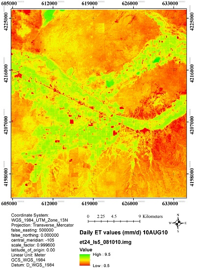
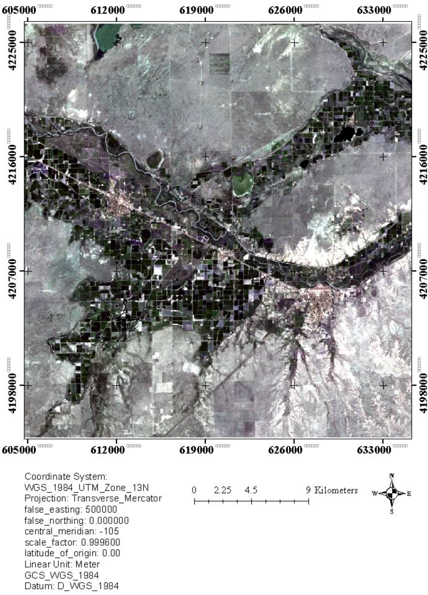
2.1. Study Area

The research was carried out at the Colorado State University (CSU) Arkansas Valley Research Center (AVRC) near Rocky Ford, in southeastern Colorado. The study area has geographic coordinates 38°02'N, 103°41'W (61,552.876 m Easting, 42,103,331.195 m Northing, UTM, Figure 1), with an elevation of 1274 m above mean sea level (amsl). The rainfall received annually in the area averages about 300 mm, with 65% falling in May through September. This amount of rainfall is not enough to sustain the growth of most agricultural crops, which makes irrigation necessary. Dry areas surround the irrigated fields as the region is of a semi-arid nature (Figure 1). The average temperature in summer is 23.6 °C, and the average daily maximum temperature is 33.0 °C. The average relative humidity in the mid-afternoon is 25% in summer, and average wind speed is 4.4 m·s−1. All these conditions make afternoon advection in the area a common occurrence.
Two alfalfa fields were used for the study. They were irrigated using a furrow irrigation system supplied by siphons and a head ditch. Field A was rectangular; 160 m by 250 m, and Field B was triangular (right-angled, with base 110 m and perpendicular length of 230 m). Close to the center of Field A was a large monolithic weighing lysimeter (3 m × 3 m × 2.4 m deep), and a smaller monolithic lysimeter (1.5 m × 1.5 m × 2.4 m) was in Field B. A monolithic lysimeter contains an undisturbed soil core that has a similar soil structure (soil layering and properties) as the surrounding field [17]. Both fields were equipped with net radiometers (REBS, Campbell Scientific International (CSI), Logan, UT, USA). There were also infrared thermometers (IRT, Apogee model S1-111, CSI, Logan, UT, USA) to measure crop radiometric surface temperature. Soil heat flux plates (REBS model HFT3, CSI, Logan, UT, USA) were buried 10 cm in the ground, along with soil temperature and soil volumetric water content sensors at locations near the net radiometer with their measurements used in the calculation of soil heat flux.

2.2. Landsat Satellite Datasets and Processing

Landsat 5 Thematic Mapper (TM) and Landsat 7 Enhanced Thematic Mapper Plus (ETM+) satellite images were downloaded from the USGS Earth Explorer site (http://edcsns17.cr.usgs.gov/NewEarthExplorer/) for the 2010–2012 growing seasons. The temporal resolution (or revisit period) is 16 days for both satellites, with alternating overpass. Therefore, if cloud cover or the swaths of missing data for Landsat 7 do not affect images, the number of days between overpasses becomes 8. Both satellites provide images at a spatial resolution of 30 × 30 m in the visible and near infrared portions of the electromagnetic spectrum. The thermal infrared band for Landsat 5 has a spatial resolution of 120 m × 120 m while Landsat 7 has a spatial resolution of 60 m × 60 m.
Figure 1. Study area, irrigated fields surrounded by dry areas.
Remotesensing 07 15046 g001
While the research fields may have been relatively small, at least one uncontaminated thermal pixel for Landsat 5 could be found, and even more for Landsat 7. However, to further rule out the possibility of pixel contamination, a thermal pixel sharpening process, based on documented evidence that there is a relationship between percentage of ground cover and surface temperature [18], was carried out. Due to the fact that percentage of ground cover is highly correlated to NDVI, the latter was used as a surrogate for ground cover, as has been used in several sharpening approaches [19,20,21].
The process was carried out for each image because the relationship between ground cover and surface temperature is not constant but varies with weather, surface conditions and land cover type [22]. This process involved selecting 25 pixels from fields large enough to have uncontaminated pixels from across the image or its subset. The pixels selected varied from partial to full cover. From each pixel selected, the NDVI, surface temperature and reflectance for bands 5 and 7 were noted. The 25 pixels were then randomly divided into training and testing datasets; 15 pixels for the training dataset and 10 for the testing dataset.
The training dataset was then used to establish the relationship between the NDVI and the radiometric surface temperature. The equation relating the NDVI to radiometric surface temperature was then used to estimate surface temperature, using the NDVI from the testing dataset, and the estimated temperature was compared with the radiometric surface temperature. The deciding factor on the appropriateness of the regression was the ratio RMSE/σ where σ is the standard deviation of Ts from the testing dataset and RMSE is the root mean square error from the comparison. A value of approximately 1 indicates poor agreement between estimations and observations, while values <0.5 means the equation is capable of estimating good values and estimations are in satisfactory agreement with observations [23]. In this study, if RMSE/σ was less than 0.5, the relationship was used for the whole scene to process a new image for surface temperature at a refined resolution of 30 m × 30 m. Table A1 in appendices show the equations used to relate NDVI to surface temperature.
As the lysimeter area was 9 m2 and the Landsat pixel is 900 m2, for these to be comparable, an effort was made to ensure that on the days of analysis, the conditions in the lysimeter were representative of the entire field. A logbook was used to record the crop heights in the lysimeter and also for the surrounding field. A neutron probe was used to measure soil water content or moisture inside and outside the lysimeter, ensuring that there was no water stress both in the lysimeter and the larger field on the days of analysis.

2.3. Evaluating SEBAL Performance under Advective Conditions

To evaluate the performance of the SEBAL model, comparison was made between the SEBAL-modeled alfalfa ET and the alfalfa ET measured using lysimeters in Fields A and B. The comparison was made for hourly and daily time-steps. Several indicators were used to measure the model performance in estimating ET, and these were: Coefficient of determination (R2), Mean Bias Error (MBE) [24,25], Root Mean Square Error (RMSE) [24] and the Nash-Sutcliffe Coefficient of Efficiency (NSCE) [26,27].

2.4. Development and Validation of the Modified SEBAL Model (SEBAL-A)

2.4.1. Data Requirement for Model Development

The SEBAL-A model was developed under standard surface conditions and the criteria for standard conditions were alfalfa of height 40–60 cm, completely covering the ground, and not short of water. The use of standard surface in the development of the model was done with the aim of validating SEBAL-A on the same standard surface before using it on non-standard surfaces, as a test for transferability. The non-standard surface conditions include different crops and moisture conditions [28]. Processed Landsat 5 and 7 images from 2010 to 2012 were selected for cases where the field satisfied the standard conditions. A crop field log that included crop height was used to select the days when the alfalfa was 40–60 cm tall. The SEBAL-based EF was used to determine whether or not the alfalfa was water-stressed, and images when the fields of study had EF > 0.96 were selected as satisfying the standard surface conditions. Soil moisture measurements using the neutron probe taken around the lysimeter were also used to confirm that there were no water-stress conditions.
For model development, available data were split into calibration and testing (validation) datasets. To have enough data for both training and testing processes, non-overpass days were used as training dataset, then overpass days as testing dataset. For the training dataset, five days prior to each of the satellite overpass days were used. This assumed that these five days had about the same standard conditions as the day of satellite overpass. This assumption was valid unless within the five days there was irrigation or rainfall, in which case the day of irrigation or rainfall event and the days prior would be discarded. The images on the overpass days were then used to validate the model under standard conditions.

2.4.2. Description of the Model Development Process

The development of the SEBAL-A model involved the parameterization of advection and incorporating it into the original SEBAL ET24 sub-model. The variables required for the estimation of daily-advected heat energy were minimum and maximum temperatures, wind run, and relative humidity.
To estimate advection, a semi empirical approach was used which is based on the concept of advective enhancement on evaporation [29]. The concept states that evaporation (E) can be expressed as the sum of equilibrium evaporation (Eeq) due to available energy at the site, and enhanced evaporation (Ead) due to extra energy brought in by advection.
E = Eeq + Ead
The same concept was illustrated using Penman’s expression of potential ET [30] as shown in Equation (13).
λET p = Δ Δ + γ Q n + λ γ Δ +   γ E a
where λ is the latent heat of vaporization (J·kg−1), γ is the psychrometric constant, Δ is the slope of the temperature–saturation vapor pressure relationship (kPa·°C1), Qn (W·m−2) is the available energy and Ea (W·m−2) is the drying power of the atmosphere. The first term in Equation (13) is the equilibrium ET, which is ET resulting from available energy at the surface (Rn − G). The second term represents ET resulting from advection, which is also referred to as “imposed ET” (ETimp) [31].
In most cases Ea, which is the drying power of the atmosphere, is calculated as a function of horizontal wind speed measured at a certain height (e.g., 2 m) and the vapor pressure deficit [30]:
Ea = f (u) × (es − ea)
where es and ea are saturation and actual vapor pressures (kPa), respectively, and f (u) is the wind function. Different approaches have been suggested for the wind function, some being empirical linear approximations [32], others theoretical, and include a roughness parameter [33,34]. One was specifically developed for alfalfa in Idaho, which was a linear function of mean horizontal wind speed [35].
In this study, three approaches were used to compare their accuracy in estimating the amount of advection to be incorporated into the SEBAL model. The first approach was to use the wind function as developed by Stigter [34], Equation (15).
f ( u ) = 8 ( 1 + U 100 ) [ l n ( z 2 d ) z o m ] 2
where z2 is the height of measurement, d (m) is the zero-plane displacement height and zom (m) is the roughness length for momentum transfer. Both d and zom (m) can be estimated based on the height of the standing crop (h), with d estimated to be 0.67h and zom to be 0.123 h. For regional estimation of ET, measuring the crop height represented in each pixel would be impossible. In SEBAL, zom is determined using satellite-based NDVI values for each pixel, and the relationship is shown as:
z o m = exp ( a   ×   N D V I + b )
where “a” and “b” are coefficients empirically obtained by relating satellite-obtained NDVI, from a sample of pixels in the image, to measured heights of vegetation in the area corresponding to the sampled pixels. The values of “a” and “b” are location specific and depend on the vegetation. However, variation of the coefficients may be less with similar vegetation (e.g., agricultural as opposed to forests).
The second approach was to modify Equation (15) to include a temperature parameter, and, in this case, daily mean temperature was used.
f ( u ) = β ( T m e a n ) ( 1 + U 100 ) [ l n ( z 2 d ) z o m ] 2
where Tmean is the daily mean temperature, which is the average of the maximum and minimum temperatures (Tmax and Tmin, respectively), and U is the afternoon representation of wind run in km·d−1. The value of β was determined by comparing the model ET to lysimeter-measured ET from the calibration dataset, and using solver with an objective of obtaining the minimum RMSE.
The third approach used daily temperature extremes instead of daily mean temperature as shown in Equation (18).
f ( u ) = β ( T m a x 20   ° C ) ( T m i n 10   ° C ) ( 1 + U 100 ) [ l n ( z 2 d ) z o m ] 2
where Tmax and Tmin are the day’s maximum and minimum temperatures (°C), respectively. Determining the value of β involved the following steps:
  • Using Equation (12), the advected energy (Ead) was determined as the difference between total latent energy, which is the energy equivalent of the lysimeter ET and the energy due to net solar radiation, which was measured using a net radiometer on site.
  • The determined Ead was then equated to the product of VPD (es − ea) and the wind function, es and ea were calculated using weather stations parameters recorded at the station, and for f(u), Equations (17) and (18) were used in turn with β being the only unknown in the equation.
  • To determine β, a set of the modeled ET was compared to lysimeter ET, from the calibration dataset, and using the solver function in MS Excel with an objective of obtaining the minimum RMSE.
The value of β is partly dependent on the selected denominators for Tmax and Tmin, which are 20 °C and 10 °C, respectively. Observed data were used to select the denominators. On the Tmax, surface radiometric temperatures of the standard conditions observed averaged around 294 K (20.85 °C), and assuming insignificant temperature change due to irradiative energy on well-watered surfaces, advection of air warmer than the surface would enhance ET, hence the selection of 20 °C.
The model performed better when Equation (18) was used than when Equations (17) and (15) were used, and the value of β that achieved the minimum RMSE was 8.0023. The better performance of Equation (18) seemed to have resulted from two factors. Firstly, that in advection, air temperature does not only determine the magnitude of VPD (which represents the capacity of air to accept vapor from the evaporation surface), but it also determines the amount of heat energy that is brought onto the evaporating surface, thus a wind function with both wind and temperature variables as shown in Equations (17) and (18) has more physical meaning.
Also, the day’s extreme temperatures, rather than the mean temperature, seem to give a more accurate estimate of advection. The maximum air temperature gives an estimate of the sensible heat energy of the air brought onto the evaporating surface on the advective afternoons. The minimum air temperature, depending on its magnitude, may give an indication of the possibility of having nighttime ET. Including the minimum temperature distinguishes conditions where the temperature might be high enough for nighttime ET to take place. It must be noted that in cases where the minimum temperature was below 10 °C, a minimum of 10 °C was used, so as to achieve the fraction unity.
Equation (18), accounts for the aerodynamic characteristics, which are influenced by surface roughness conditions. Although the equation was developed using data obtained during standard surface conditions, it is expected that Equation (18) would be transferable to different crop surfaces because of the roughness component. However, stomatal resistance was not factored in the equation, with the assumption that the EF would account for it.
When Ea and subsequently Ead had been determined, Ead was then introduced into the ET24 sub-model of SEBAL, and Equation (11) was modified to be Equation (19) in SEBAL-A:
ET 24   = 86 , 400   ×   E F   × ( R n 24   +   λ E a d ) λ   ×   ρ w

2.5. Model Validation

The validation of the SEBAL-A model involved comparing the alfalfa daily ET estimated using SEBAL-A to alfalfa daily ET measured using lysimeters. The statistical indicators used to evaluate the model performance were R2, MBE, RMSE and NSCE. The performance of SEBAL-A was also compared to that of the original SEBAL to determine if there was any improvement.

3. Results and Discussions

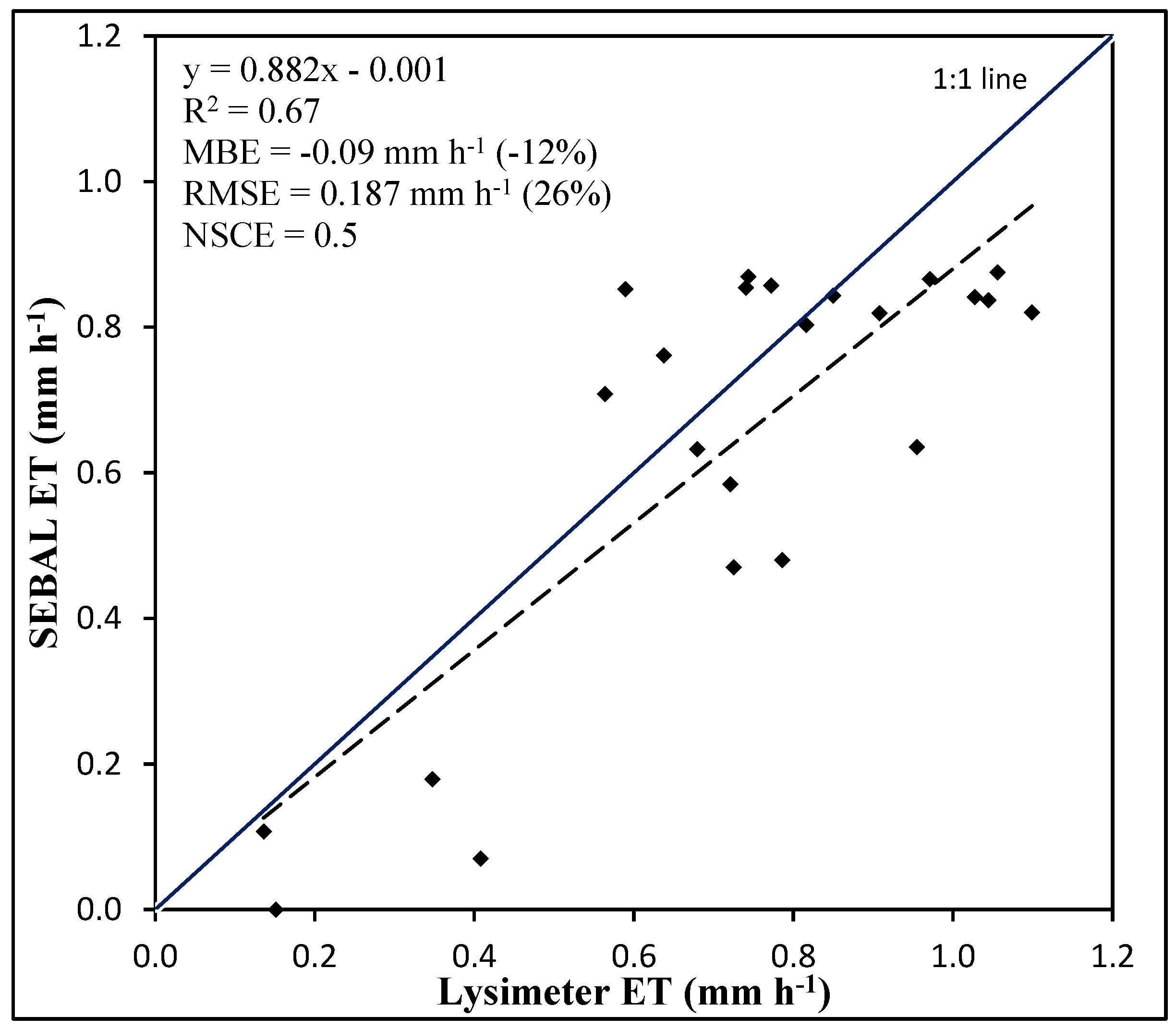
3.1. Evaluation of SEBAL under Advective and Non-Advective Conditions

When the hourly alfalfa ET estimated using SEBAL was compared with measured ET using the large monolithic weighing lysimeter, the resulting MBE was −0.09 mm·h−1 (−12%), which on average showed only a slight underestimation of ET. The comparison is illustrated graphically in Figure 2. The RMSE was 0.187 mm·h−1 (26%), and the NSCE was 0.5, which was within the acceptable range of model performance.
Figure 3 shows results for the daily ET from the original SEBAL compared to lysimeter daily ET values. Figure 3 has three fewer data points as in three of the days of analysis, there was activity (e.g., irrigation, harvesting) in the lysimeter or field after time of satellite overpass, and therefore the daily data could not be used for analysis. The results indicate that there was a significant underestimation of daily ET, with MBE of −2.6 mm·d−1 (−32%) and RMSE of 3.18 mm·d−1 (39%). The NSCE was −0.07, which indicates an unacceptable performance of the model in estimating daily alfalfa ET for irrigated alfalfa under standard surface conditions in southeastern CO. While the original SEBAL model seems appropriate in estimating hourly ET (NSCE = 0.5), during the time of satellite overpass (which was between 10.20 and 10.30 am MST), it was found to be unsuitable for estimating daily ET (NSCE = −0.07). The reason SEBAL would be suitable to estimate ET on hourly basis and not suitable on daily basis could be due to the use of EF in extrapolating instantaneous ET to daily values. The extrapolation assumes that the EF at the time of satellite overpass remains constant throughout the day, which is sometimes not the case with occurrence of afternoon advection, which was usually the case in most summer afternoons in the semi-arid area around Rocky Ford, CO. A similar observation was made, that on advective days SEBAL may underestimate ET [9]. Gowda et al. [36] reported an average SEBAL accuracy of 85% for a single day, while Trezza [11] found the error for SEBAL to range from 2.7% to 35%, with 18.2% being the overall average error.
Figure 2. Comparing SEBAL-modeled and Lysimeter-measured hourly alfalfa ET at time of satellite overpass.
Remotesensing 07 15046 g002
It was also noticed that there was some discrepancy between modeled and measured ET on both hourly and daily ET with low ET, mostly when the fields had low vegetation cover. This could indicate that the original SEBAL model may not be appropriate for ET estimation in less vegetated surfaces because of surface heterogeneity. SEBAL is a one-source model, i.e., the heterogeneous surface is represented as a single layer [37], and the energy balance components are determined as coming from one source. Hipps and Kustas [38] mentioned that there is a problem when a heterogeneous surface is represented as a single source as soil has a significant influence on the surface energy balance. Also, with less cover the H and G components of the energy balance are large and, therefore, play a significant role in the final ET. Thus, if H and G are inaccurately estimated, errors will be transferred onto the final estimation of ET values. However, with vegetated, well-irrigated areas, H and G are closer to zero and, therefore, are of limited significance.
Figure 3. Comparing the original SEBAL and Lysimeter-measured daily alfalfa ET in southeastern Colorado.
Remotesensing 07 15046 g003

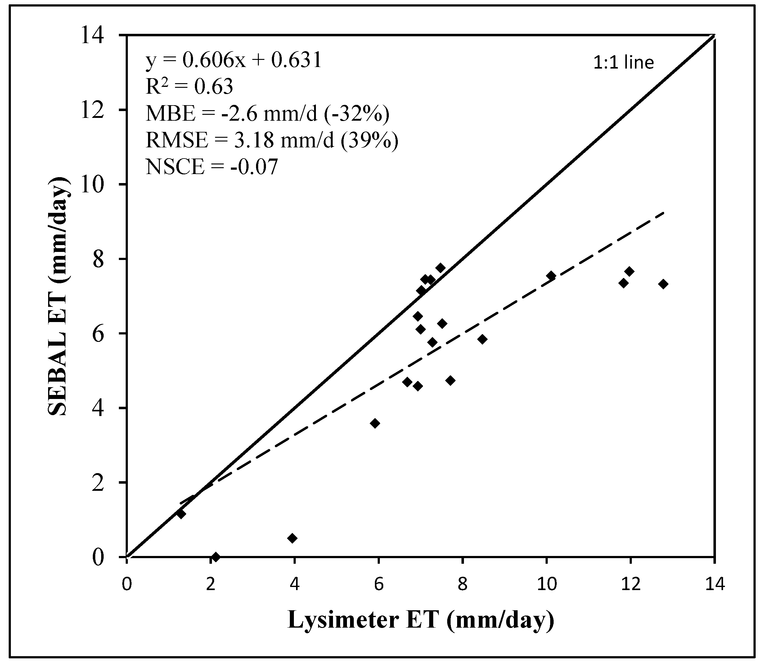
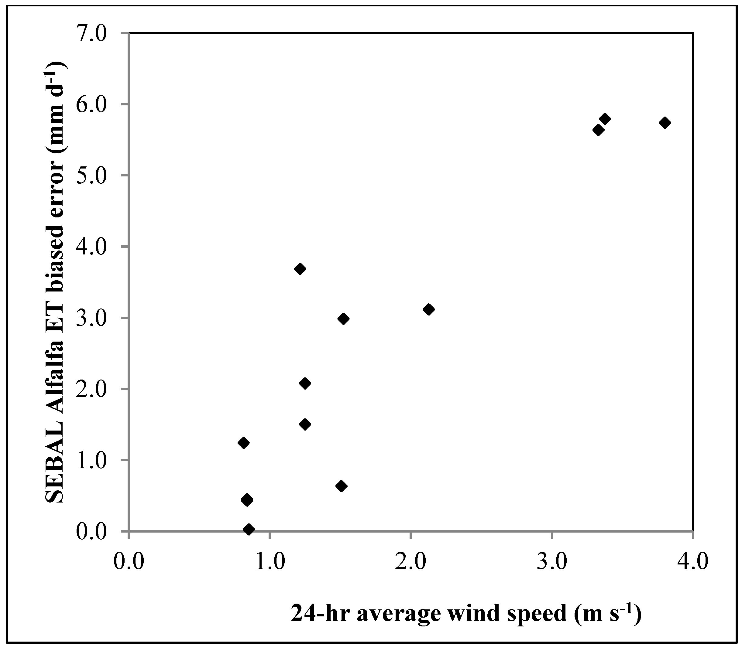
3.2. The Advective Effects of Wind, Humidity and Air Temperature

High wind speed, high air temperature and low humidity signal the occurrence of advection. These parameters have been termed advection indicators [39]. Brakke et al. [40] mentioned wind speed as one of the conditions that contribute to regional advection. In this paper, 2010 alfalfa data from the Colorado State University (CSU) Arkansas Valley Research Center (AVRC) near Rocky Ford was used to illustrate the relationship between wind speed and error incurred by the SEBAL model in estimating daily alfalfa ET, and the results are as shown in Figure 4 and Figure 5. Figure 4 used average wind speed over a 24-hr day, while Figure 5 used the afternoon average wind speed (between noon and when Rn decreases to 0), when the air is warmer and drier, hence more advected energy. There seemed to be a stronger correlation with the latter, suggesting that the errors in the original SEBAL model were mostly due to the afternoon advection occurrence, which the SEBAL model could not account for.
Figure 4. Relationship between 24-hr average wind speed and SEBAL model alfalfa ET error.
Remotesensing 07 15046 g004
Figure 5. Relationship between afternoon wind speed averages and SEBAL alfalfa ET model error.
Remotesensing 07 15046 g005
The shape of the curve is also worth noting, especially in Figure 5, where at low wind speeds (<1.5 m·s−1), the errors seem to be independent of wind speed, but for winds greater than 1.5 m·s−1, there was an obvious relationship between wind speed and SEBAL ET estimation errors, with the error increasing with increasing wind speed until around 4 m·s−1 when increasing wind speed did not result in increased error. The presence of error for wind speed less than 1.5 m·s−1 may have been a result of local rather than regional advection. Usually, local advection is a small portion of the total advection in cases where both forms occur, or about a fifth of the total advection effect on ET, and the local advection is usually unrelated to wind speed [40]. It may be for that reason, therefore, that at low wind speeds with drier and warm air there could still be some error observed on estimated ET.
The leveling off of errors in the estimation of ET at about 4 m·s−1 in Figure 5 could be due to the fact that the higher wind speed may result in a higher evaporative demand which the alfalfa cannot cope with, and therefore resulting in a response by alfalfa in the form of reduced stomatal conductance. There is an inverse relationship between canopy moisture conductance and saturation deficit at the canopy surface [41]. This may explain the plateau (asymptote) of SEBAL ET error at high wind speeds.
Table 1 shows results from the SEBAL model, indicating that there was less error on days when the average relative humidity was close to and above 70%. On days 15 June 2010, 10 August 2010 and 5 August 2011, when the humidity was high, the absolute errors on ET were less than 10%. This is in agreement with Gentine et al. [7] that under conditions of higher relative humidity, the evaporative fraction is more likely to be constant, and, therefore, the extrapolation of instantaneous ET to daily ET would be more accurate. However, on days with low humidity (e.g., 22 May 2010, 20 June 2012 and 22 July 2012) when the average relative humidity was less than 45%, for example, the error was consistently above 30% and reaching up to 40%, when low humidity was accompanied by higher wind speed.
Table 1. Average weather conditions, field measurements and SEBAL model performance on days of satellite overpass.
DateTa (°C)RH (%)U (m·s−1)h (cm)Model error (%)Night ET (mm)
24-hrAfternoon
6/15/2010 (A)19.266.71.43.2309.30.4
7/1/2010 (A)24.847.73.33.766−35.51.1
8/18/2010 (A)24.355.50.80.955−2.70.4
5/6/2010 (A)16.240.74.38.443−15.00.7
5/22/2010 (A)23.2283.85.360−35.61.4
8/10/2010 (A)23.069.10.91.0500.60.0
8/26/2010 (A)22.146.61.82.612−34.10.4
6/15/2010 (B)18.870.11.42.5104−14.70.2
5/6/2010 (B)15.742.93.66.860−28.21.0
5/22/2010 (B)22.132.33.04.092−40.32.1
8/10/2010 (B)23.763.51.01.0*2.10.2
6/18/2011 (A)22.1502.43.725−14.70.5
7/4/2011 (A)24.449.81.12.770−21.00.1
8/21/2011 (A)23.762.91.31.770−11.70.3
6/18/2011 (B)22.250.32.43.518−32.20.7
8/5/2011 (B)23.964.30.90.948−3.70.6
6/4/2012 (B)22.646.62.75.225−22.40.4
6/4/2012 (A)22.447.72.85.632−26.20.6
6/20/2012 (A)23.143.63.43.576−32.21.7
7/22/2012 (A)27.036.41.62.853−39.81.1
Note: Ta is air temperature, U is the wind speed, RH is relative humidity and h is the crop height. The A and B after the dates indicate the field from which the data was obtained, either Field A or B.
There is some complexity as to how these advection indicators interact with each other and also with the evaporating surface in order to determine how much latent heat flux will result from the advected energy. For instance, 22 May 2010 was the day with the highest ET underestimation observed. From analysis of the weather data, also shown in Table 1, this was due to the high wind speed of 3–4 m·s−1 and a low relative humidity of about 30%. This resulted in SEBAL underestimating ET by about 40%. The opposite occurs on 10 August 2010, where there was minimal error in ET estimation, and the conditions prevailing were non-advective, with the average wind speed being 0.9 m·s−1 and a relative humidity of 69%.
On 4 July 2011, the 24-hour average wind speed was low (1.1 m·s−1) and RH of about 50%, but the SEBAL model underestimated ET by 21%. However, Table 1 also shows that the afternoon average wind speed was 2.7 m·s−1, and therefore the wind was capable of transporting substantial sensible heat from surrounding areas, hence the large error. This observation shows that the afternoon wind speed is the more appropriate indicator of advection than the 24-hour average wind speed as was earlier discussed. A similar observation was made on 22 July 2012, where a 40% underestimation of ET by SEBAL was observed, with a 24-hour average wind speed of 1.6 m·s−1. However, the afternoon average wind speed was 2.8 m·s−1, and afternoon average temperature and RH were 34 °C and 24%, respectively (not shown in table), which suggest advective conditions.
The day of 6 May 2010 was a windy day, especially in the afternoon with an average wind speed of about 7 m·s−1, but the ET error was less than 30%, which was less than other days with lower wind speed and higher RH. This could have been due to the lower temperatures on the day compared to the other days, with mean temperature being 16 °C, thus the air brought onto the field was cool and therefore had less sensible heat energy.

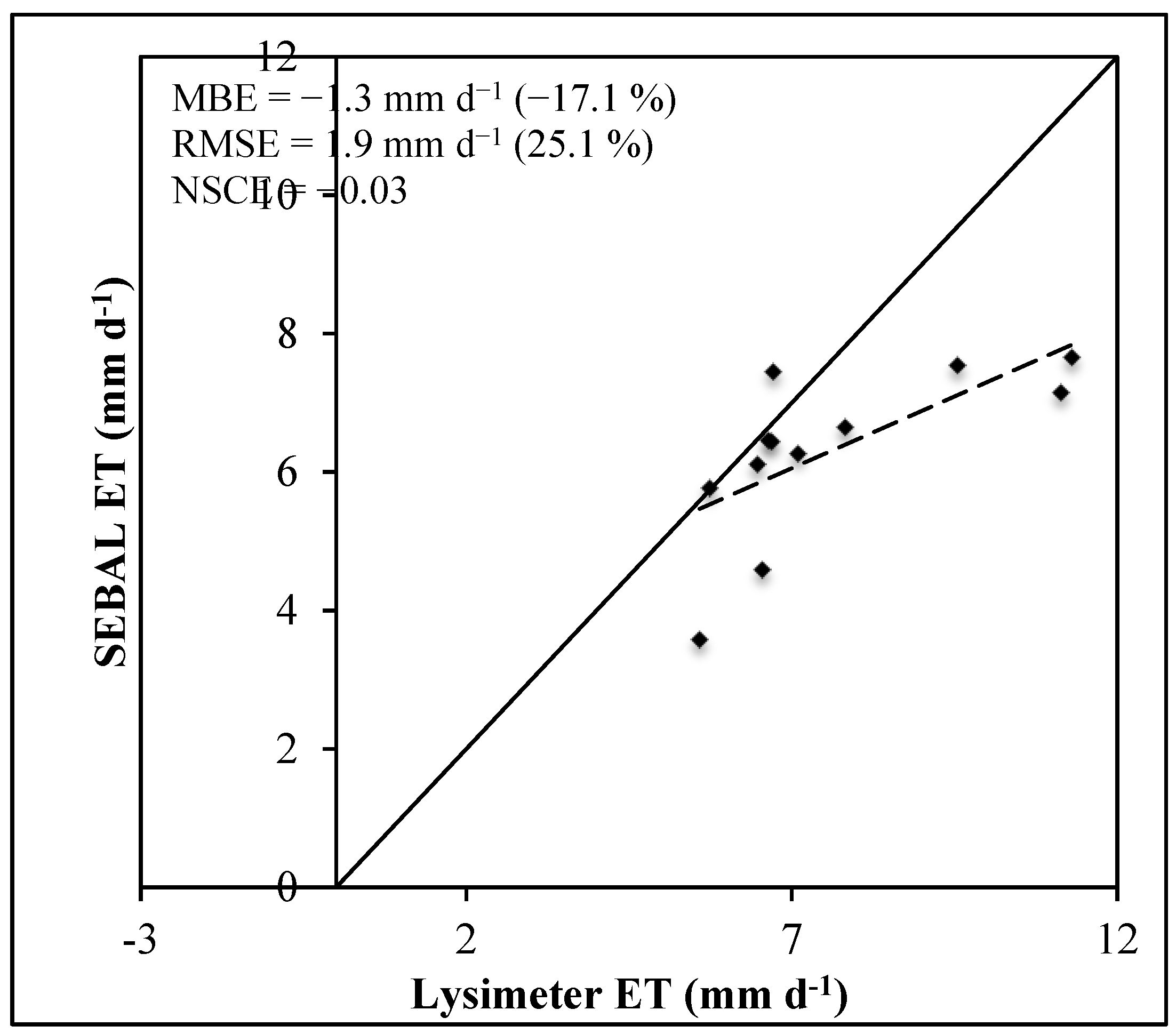
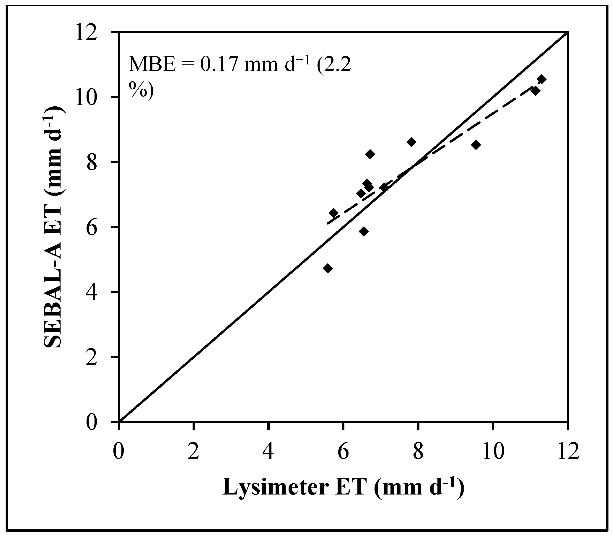
3.3. Development and Validation of SEBAL-A

After the SEBAL-A model was developed, as earlier described, it was tested using Landsat 5 and 7 images for overpass days under standard conditions. Using Equation (18) to determine the wind function, the drying power of the air (Ea) was determined and subsequently the advected energy (Ead). The Ead was then included in the ET24 sub-model, as given in Equation (19).
Table 2 shows the results of the modification, and compares the errors in the modified SEBAL (SEBAL-A) model with the original SEBAL. On average, the original SEBAL underestimated Alfalfa ET by 17%, with underestimations of up to 38%, while SEBAL-A resulted in an average overestimation of about 2.2%, with errors less than 20% except on 5 August 2010 which had an ET error of 24%. Table 2 shows statistics for both the original and SEBAL-A, with the latter showing significant improvement over the original SEBAL. The Mean Bias Error of −1.3 mm·d−1 (−17.1%) in the original SEBAL was reduced to 0.17 mm·d−1 (2.2%) with SEBAL-A. The Root Mean Square Error was reduced from 1.9 mm·d−1 (25.1%) to 0.83 mm·d−1 (10.9%). An NSCE of −0.03, which suggested that the SEBAL model was unsuitable to estimate daily ET, was improved to a good value of 0.81 with SEBAL-A.
Figure 6 and Figure 7 show graphs of alfalfa ET estimated using the original SEBAL and SEBAL-A, respectively, compared to lysimeter-measured alfalfa ET. SEBAL-A ET estimates compared very well with the lysimeter ET values, whilst the original SEBAL significantly underestimated ET. The underestimation was largest for higher ET values, where there was more advection. For SEBAL-A, most of the points were close to the 1:1 line. The ability of SEBAL-A to reduce the MBE to close to zero is an important quality as it mostly eliminates the bias. The use of SEBAL-A will potentially result in a more accurate seasonal ET as opposed to the original SEBAL, which would underestimate seasonal ET due to cumulative ET errors.
Table 2. Performance of models on overpass days, and calculated statistics.
DateLysimeter ET (mm·d−1)SEBAL ET (mm·d−1)SEBAL-A ET (mm·d−1)
08/18/2010 (A)6.66.5 (−2.7)7.4 (12.2)
09/19/2010 (A)6.54.6 (−29.9)6.0 (−8.9)
10/05/2010 (A)5.63.6 (−38.9)4.8 (−13.6)
08/05/2011(A)6.77.5 (10.9)8.3 (24.1)
05/06/2010 (A)7.86.7 (−15.0)8.7 (11.8)
05/22/2010 (A)11.17.2 (−35.6)10.4 (−6.5)
08/10/2010 (A)5.75.8 (0.6)6.5 (13.5)
08/05/2011(B)6.76.4 (−3.7)7.3 (9.4)
07/04/2011(A)9.57.5 (−21.0)8.6 (−9.5)
08/21/2011(A)7.16.3 (−11.7)7.3 (3.3)
06/20/2012 (A)11.37.7 (−32.2)10.8 (−4.7)
08/21/2011(B)6.56.1 (−5.6)7.1 (10.3)
Statistics
MBE −1.3 (−17.1)0.17 (2.2)
RMSE 1.9 (25.1)0.83 (10.9)
NSCE −0.030.81
Note: The A and B after the dates indicate the field from which the data was obtained, either Field A or B. Values in parenthesis are errors in percent.
Figure 6. Comparing SEBAL-modeled and Lysimeter-measured daily alfalfa ET under standard conditions.
Remotesensing 07 15046 g006
Figure 7. Comparing SEBAL-A and Lysimeter-measured daily alfalfa ET under standard conditions.
Remotesensing 07 15046 g007

4. Conclusions

From the results obtained from the study, it can be concluded that the SEBAL model usually underestimates ET mostly due to advection, with bias errors of up to 40% being observed for alfalfa in southeastern Colorado, U.S. The daily ET estimation resulted in larger errors than for hourly ET when SEBAL estimates were compared to lysimeter measurements. This result could be due to the occurrence of advection near Rocky Ford, Colorado, mostly in the afternoons, while hourly ET is estimated around the satellite overpass time, which is between 10:20 a.m. and 10:30 a.m. Mountain Standard Time (MST).
Another observation was that the original SEBAL model incurred more error in estimating ET when there was less vegetation cover. There are several possible explanations to this observation. One of them being that the SEBAL model is a single-source model, assuming that all the fluxes are from a single uniform source (big leaf approach). However, with low vegetation cover, where the soil is exposed, a two-source approach is theoretically more accurate and appropriate. Another reason for higher accuracy with full vegetation cover is that H is usually small, and, therefore, even if H is inaccurately estimated, it will have less impact on the final LE value. However, with low vegetation cover, and/or water stressed vegetation, both G and H may be large and errors in their determination may significantly affect the accuracy of LE as a residual of the surface energy balance. The estimation of H involves the selection of extreme pixels, which is a subjective exercise, and depends on several factors, which include the presence of appropriate pixels.
When the ET24 sub-model for SEBAL was modified by including modeled advection (SEBAL-A model), the ET estimation was significantly improved for advective conditions. Advective conditions are a common occurrence in arid and semi-arid regions, and the modification of the SEBAL model improves the estimation of ET in regions where there is advection.
However, the significant characteristic of SEBAL-A is its ability to account for advection by using minimum weather data. This means the model can be used under advective conditions even where hourly weather data may not be available. Most models require weather data at least on a hourly basis to be able to account for advection; SEBAL-A, on the other hand, only uses minimum and maximum temperatures, daily wind run and vapor pressure to achieve that.

Acknowledgements

We would like to extend our appreciation to CSU-AVRC Director Michael Bartolo, and staff; Lane Simmons, Jeff Davidson and Kevin Tanabe, for their assistance with field activities and data collection. We would also like to thank students in the Civil and Environmental Engineering Department at CSU who were involved in collecting data used in this work; Evan Rambikur, Abhinaya Subedi and Stuart Joy (who were funded by Colorado Agricultural Experiment Station and USDA NIFA). We also thank Tom Trout and Jay Ham as well as anonymous reviewers, for their comments to improve the quality of this work and journal article, respectively. Last but not least, we thank the Institute of International Education (IIE) through the Fulbright Science and Technology Program for funding part of this work, including publishing costs.

Author contributions

Mcebisi Mkhwanazi and José L. Chávez set out the experimental plan. Mcebisi also processed remote sensing data, analyzed them together with lysimeter data. José Chávez provided guidance and review on the progress of the study. José Chávez and Allan Andales provided quality controlled large weighing lysimeter data from CSU-AVRC. Mcebisi Mkhwanazi wrote the manuscript and all co-authors were involved in its review.

Conflicts of Interest

The authors declare no conflict of interest.

Appendix

Table A1. Equations relating NDVI and radiometric surface temperature.
DateEquationRMSE/σ
05/06/2010y = −29.580x + 318.510.27
05/22/2010y = −23.452x + 319.050.19
06/15/2010y = −17.154x + 311.000.11
06/18/2010y = −25.140x + 324.610.35
07/01/2010y = −23.876x + 319.450.26
07/04/2010y = −26.751x + 319.720.11
08/10/2010y = −19.177x + 314.490.18
08/18/2010y = −22.060x + 317.920.28
08/26/2010y = −32.753x + 323.800.36
08/05/2011y = −20.854x + 315.940.19
08/21/2011y = −21.436x + 315.840.15
06/20/2012y = −23.061x + 311.510.17
07/22/2012y = −31.111x + 317.430.29

References

  1. Bastiaanssen, W.G.M.; Menenti, M.; Feddes, R.A.; Holtslag, A.A.M. A remote sensing surface energy balance algorithm for land (SEBAL). 1. Formulation. J. Hydrol. 1998, 212–213, 198–212. [Google Scholar] [CrossRef]
  2. Allen, R.G.; Tasumi, M.; Trezza, R. Satellite-based energy balance for mapping evapotranspiration with internalized calibration (METRIC) model. ASCE J. Irrig. Drain. Eng. 2007, 133, 380–394. [Google Scholar] [CrossRef]
  3. Bastiaanssen, W.G.M.; Noordman, E.J.M.; Pelgrum, H.; Davids, G.; Thoreson, B.P.; Allen, R.G. SEBAL Model with remotely sensed data to improve water resources management under actual field conditions. J. Irrig. Drain. Eng. 2005, 131, 85–93. [Google Scholar] [CrossRef]
  4. Allen, R.G.; Tasumi, M.; Morse, A. Satellite-based evapotranspiration by energy balance for western states water management. In Proceedings of the World Water and Environmental Resources Congress, Anchorage, AL, USA, 15–19 May 2005; pp. 1–18.
  5. Allen, R.; Irmak, A.; Trezza, R.; Hendrickx, J.M.H.; Bastiaanssen, W.; Kjaersgaard, J. Satellite-based ET estimation in agriculture using SEBAL and METRIC. Hydrol. Process. 2011, 25, 4011–4027. [Google Scholar] [CrossRef]
  6. Hoedjes, J.C.B.; Chehbouni, A.; Jacob, F.; Ezzahar, J.; Boulet, G. Deriving daily evapotranspiration from remotely sensed instantaneous evaporative fraction over olive orchard in semi-arid Morocco. J. Hydrol. 2008, 354, 53–64. [Google Scholar] [CrossRef]
  7. Gentine, P.; Entekhabi, D.; Polcher, J. The diurnal behaviour of evaporative fraction in the soil-vegetation-atmospheric boundary layer continuum. J. Hydrometeorol. 2011, 12, 1530–1546. [Google Scholar] [CrossRef]
  8. Gowda, P.H.; Howell, T.A.; Paul, G.; Colaizzi, P.D.; Marek, T.H. SEBAL for estimating hourly ET fluxes over irrigated and dryland cotton during BEAREX08. In Proceedings of the World Environmental and Water Resources Congress, Palm Springs, CA, USA, 22–26 May 2011; pp. 2787–2795.
  9. Singh, R.K.; Irmak, A.; Irmak, S.; Martin, D.L. Application of SEBAL Model for mapping evapotranspiration and estimating surface energy fluxes in South-Central Nebraska. J. Irrig. Drain. Eng. 2008, 134, 273–285. [Google Scholar] [CrossRef]
  10. Bastiaanssen, W.G.M. Regionalization of Surface Flux Densities and Moisture Indicators in Composite Terrain: A Remote Sensing Approach under Clear Skies in Mediterranean Climates. Ph.D. Dissertation, CIP Data Koninklijke Bibliotheek, Den Haag, The Netherlands, 1995. [Google Scholar]
  11. Trezza, R. Evapotranspiration Using a Satellite-Based Surface Energy Balance with Standardized Ground Control. Ph.D. Dissertation, Biological and Irrigation Engineering Department, Utah State University, Logan, UT, USA, 2002. [Google Scholar]
  12. Brutsaert, W.; Sugita, M. Application of self-preservation in the diurnal evolution of the surface energy budget to determine daily evaporation. J. Geophys. Res. 1992. [Google Scholar] [CrossRef]
  13. Crago, R.D.; Brutsaert, W. Daytime evaporation and the self-preservation of the evaporative fraction and the Bowen ratio. J. Hydrol. 1996, 178, 241–255. [Google Scholar] [CrossRef]
  14. Stewart, J.B. Extrapolation of evaporation at time of satellite overpass to daily totals. In Scaling up in Hydrology Using Remote Sensing; Stewart, J.B., Engman, E.T., Feddes, R.A., Kerr, Y., Eds.; Wiley: Chichester, UK, 1996; pp. 245–255. [Google Scholar]
  15. Lhomme, J.P.; Elguero, E. Examination of evaporative fraction diurnal behavior using a soil-vegetation model coupled with a mixed-layer model. Hydrol. Earth Syst. Sci. 1999, 3, 259–270. [Google Scholar] [CrossRef]
  16. Irmak, A.; Allen, R.G.; Kjaersgaard, J.; Huntington, J.; Kamble, B.; Trezza, R.; Ratcliffe, I. Operational remote sensing of ET and challenges. In Evapotranspiration—Remote Sensing and Modeling; Irmak, A., Ed.; InTech: Rijeka, Croatia, 2012; Available online: http://www.intechopen.com/books/evapotranspiration-remote-sensing-and-modeling/operational-remote-sensing-of-et-and-challenges (accessed on 28 September 2015). [CrossRef]
  17. Marek, T.; Piccinni, G.; Schneider, A.; Howell, T.; Jett, M.; Dusek, D. Weighing lysimeters for the determination of crop water requirements and crop coefficients. Appl. Eng. Agric. 2006, 22, 851–856. [Google Scholar] [CrossRef]
  18. Badeck, F.W.; Bondeau, A.; Bottcher, K.; Doktor, D.; Lucht, W.; Schaber, J.; Sitch, S. Responses of spring phenology to climate change. New Phytol. 2004, 162, 295–309. [Google Scholar] [CrossRef]
  19. Woonsook, H.; Gowda, P.H.; Howell, T.A.; Paul, G.; Hernandez, J.E.; Basu, S. Downscaling surface temperature image with TsHARP. In Proceedings of the 5th National Decennial Irrigation Conference, Phoenix Convention Center, Phoenix, AZ, USA, 5–8 December 2010. [CrossRef]
  20. Allen, R.G.; Robison, C.W.; Garcia, M.; Kjaersgaard, J. Enhanced resolution of evapotranspiration by sharpening the Landsat thermal band. In Proceedings of the ASPRS-Pecora 17 Fall 2008 Conference, Denver, CO, USA, 18–20 November 2008; Available online: http://www.researchgate.net/publication/255665728 (accessed on 28 September 2015).
  21. Agam, N.; Kustas, W.P.; Anderson, M.C.; Li, F.; Colaizzi, P.D. Utility of thermal image sharpening for monitoring field-scale evapotranspiration over rainfed and irrigated agricultural regions. Geophys. Res. Lett. 2008. [Google Scholar] [CrossRef]
  22. Karnieli, A.; Bayasgalan, M.; Bayarjargal, Y.; Agam, N.; Khudulmur, S.; Tucker, C.J. Comments on the use of the vegetation health index over Mongolia. Int. J. Remote Sens. 2006, 27, 2017–2024. [Google Scholar] [CrossRef]
  23. Kustas, W.P.; Norman, J.M. Evaluating the effects of sub-pixel heterogeneity on pixel average fluxes. Remote Sens. Environ. 2000, 74, 327–342. [Google Scholar] [CrossRef]
  24. Wilmott, C.J. Some comments on the evaluation of model performance. Bull. Am. Meteorol. Soc. 1982, 63, 1309–1313. [Google Scholar] [CrossRef]
  25. Katiyar, A.K.; Kumar, A.; Pandey, C.K.; Das, B. A comparative study of monthly mean daily clear sky radiation over India. In. J. Energy Environ. 2010, 1, 177–182. [Google Scholar]
  26. Moriasi, D.N.; Arnold, J.G.; Van Liew, M.W.; Bingner, R.L.; Harmel, R.D.; Veith, T.L. Model evaluation guidelines for systematic quantification of accuracy in watershed simulations. Trans. ASABE 2007, 50, 885–900. [Google Scholar] [CrossRef]
  27. Nash, J.E.; Sutcliffe, J.V. River flow forecasting through conceptual models part 1—A discussion of principles. J. Hydrol. 1970, 10, 282–290. [Google Scholar] [CrossRef]
  28. Mkhwanazi, M.; Chávez, J.L.; Andales, A.A.; DeJonge, K. SEBAL-A: A remote sensing ET algorithm that accounts for advection with limited data. Part II: Test for transferability. Remote Sens. 2015, 7, 15068–15081. [Google Scholar] [CrossRef]
  29. McNaughton, K.G. Evaporation and advection I: Evaporation from extensive homogenous surfaces. Quart. J. R. Met. Soc. 1976, 102, 181–191. [Google Scholar] [CrossRef]
  30. Hobbins, M.T.; Ramirez, J.A.; Brown, T.C. The complementary relationship in estimation of regional evapotranspiration: An enhanced Advection-Aridity model. Water Resour. Res. 2001, 37, 1389–1403. [Google Scholar] [CrossRef]
  31. Tolk, J.A.; Evett, S.R.; Howell, T.A. Advection influences on evaporation of alfalfa in a semiarid climate. Agron. J. 2006, 98, 1646–1654. [Google Scholar] [CrossRef]
  32. Penman, H.L. Natural evaporation from open water, bare soil and grass. Proc. R. Soc. Lond. A 1948, 193, 120–146. [Google Scholar] [CrossRef]
  33. Brutsaert, W.; Stricker, H. An advection-aridity approach to estimate actual regional evapotranspiration. Water Resour. Res. 1979, 15, 443–450. [Google Scholar] [CrossRef]
  34. Stigter, C.J. Assessment of the quality of generalized wind functions in Penman’s equations. J. Hydrol. 1980, 45, 321–331. [Google Scholar] [CrossRef]
  35. Wright, J.L. Derivation of alfalfa and grass reference evapotranspiration. In Evapotranspiration and Irrigation Scheduling, Proceedings of the International Conference, ASAE, San Antonio, TX, USA, 3–6 November 1996; Camp, C.R., Sadler, E.J., Yoder, R.E., Eds.; pp. 133–140.
  36. Gowda, P.H.; Chavez, J.L.; Colaizzi, P.D.; Evett, S.R.; Howell, T.A.; Tolk, A.T. ET mapping for agricultural water management: Present status and challenges. Irrig. Sci. 2008, 26, 223–237. [Google Scholar] [CrossRef]
  37. Chávez, J.L.; Gowda, P.H.; Howell, T.A.; Neale, C.M.U.; Copeland, K.S. Estimating hourly crop ET using a two-source energy balance model and multispectral airborne imagery. Irrig. Sci. 2009, 38, 79–91. [Google Scholar] [CrossRef]
  38. Hipps, L.; Kustas, W. Patterns and organisation in evaporation. In Spatial Patterns in Hydrological Processes: Observations and Modelling; Grayson, R.B., Biöschl, G., Eds.; Cambridge University Press: New York, NY, USA, 2000; pp. 105–122. [Google Scholar]
  39. De Bruin, H.A.R.; Hartogensis, O.K.; Allen, R.G.; Kramer, J.W.J.L. Regional Advection Pertubations in an Irrigated Desert (RAPID) experiment. Theor. Appl. Climatol. 2005, 80, 143–152. [Google Scholar] [CrossRef]
  40. Brakke, T.W.; Verma, S.B.; Rosenberg, N.J. Local and Regional Components of Sensible Heat Advection. J. Appl. Meteor. 1978, 17, 955–963. [Google Scholar] [CrossRef]
  41. Zermeño-Gonzalez, A.; Hipps, L.E. Downwind evolution of surface fluxes over a vegetated surface during local advection of heat and saturation deficit. J. Hydrol. 1997, 192, 189–210. [Google Scholar] [CrossRef]

