SEBAL-A: A Remote Sensing ET Algorithm that Accounts for Advection with Limited Data. Part II: Test for Transferability

Abstract

Because the Surface Energy Balance Algorithm for Land (SEBAL) tends to underestimate ET when there is advection, the model was modified by incorporating an advection component as part of the energy usable for crop evapotranspiration (ET). The modification involved the estimation of advected energy, which required the development of a wind function. In Part I, the modified SEBAL model (SEBAL-A) was developed and validated on well-watered alfalfa of a standard height of 40–60 cm. In this Part II, SEBAL-A was tested on different crops and irrigation treatments in order to determine its performance under varying conditions. The crops used for the transferability test were beans (Phaseolus vulgaris L.), wheat (Triticum aestivum L.) and corn (Zea mays L.). The estimated ET using SEBAL-A was compared to actual ET measured using a Bowen Ratio Energy Balance (BREB) system. Results indicated that SEBAL-A estimated ET fairly well for beans and wheat, only showing some slight underestimation of a Mean Bias Error (MBE) of −0.7 mm·d⁻¹ (−11.3%), a Root Mean Square Error (RMSE) of 0.82 mm·d⁻¹ (13.9%) and a Nash Sutcliffe Coefficient of Efficiency (NSCE) of 0.64. On corn, SEBAL-A resulted in an ET estimation error MBE of −0.7 mm·d⁻¹ (−9.9%), a RMSE of 1.59 mm·d⁻¹ (23.1%) and NSCE = 0.24. This result shows an improvement on the original SEBAL model, which for the same data resulted in an ET MBE of −1.4 mm·d⁻¹ (−20.4%), a RMSE of 1.97 mm·d⁻¹ (28.8%) and a NSCE of −0.18. When SEBAL-A was tested on only fully irrigated corn, it performed well, resulting in no bias, i.e., MBE of 0.0 mm·d⁻¹; RMSE of 0.78 mm·d⁻¹ (10.7%) and NSCE of 0.82. The SEBAL-A model showed less or no improvement on corn that was either water-stressed or at early stages of growth. The errors incurred under these conditions were not due to advection not accounted for but rather were due to the nature of SEBAL and SEBAL-A being single-source energy balance models and, therefore, not performing well over heterogeneous surfaces. Therefore, it was concluded that SEBAL-A could be used on a wide range of crops if they are not water stressed. It is recommended that the SEBAL-A model be further studied to be able to accurately estimate ET under dry and sparse surface conditions.

1. Introduction

In the article Part I [1], daily actual crop evapotranspiration (ET) estimated using the SEBAL model was compared to ET measured using a large weighing lysimeter on an alfalfa field near Rocky Ford in southeast Colorado. It was observed that SEBAL underestimated ET when there was heat advection, here defined as the horizontal transport of heat resulting from surface inhomogeneity [2], with errors of up to 40%. In arid and semi-arid areas such as Rocky Ford, where dry areas surround irrigated crops, advection and the subsequent ET underestimations from SEBAL are a common occurrence. A modification was therefore made on SEBAL by introducing an advection component into the 24-h evapotranspiration (ET₂₄) sub-model of the SEBAL ET algorithm (compare Equations (1) and (2)). The resulting modified model was named SEBAL-Advection or SEBAL-A for short. In Equation (1), the net radiation is the only source of energy that is assumed to be available for ET.

$${\text{ET }}_{24}=\frac{86,400 \times EF \times R{n}_{24}}{\lambda \times {\rho }_w}$$

(1)

In SEBAL-A, the equation was modified to include the advection component as shown below:

$${\text{ET }}_{24}=\frac{86,400\times EF\times \left(R{n}_{24}+\lambda Ead\right)}{\lambda \times {\rho }_w}$$

(2)

where 86,400 is the conversion from energy per second to per day, Rn₂₄ is the average net radiation (W·m⁻²) for the day, λ is the latent heat of vaporization used to convert the energy from W·m⁻² to mm of evaporation or vice-versa and is a function of temperature (in SEBAL, the radiometric surface temperature is used), ρ_w is the density of water in kg·m⁻³, and E_ad is the advected energy that is also available for evaporation. In Part 1, E_ad was determined as the product of a wind function and the vapor pressure deficit (e_s – e_a). A semi-empirical wind function as shown in Equation (3) was developed. The wind function includes wind and temperature parameters. Instead of using the daily average temperature as a surrogate for heat content of the transported air, minimum and maximum temperatures were used. The argument was that the average temperature masks the extent of temperature influence on afternoon advection, so the maximum temperature was used instead, and the minimum temperature indicates how the air temperature in the evening may contribute to evening/night ET.

$$f\left(u\right)=\frac{8\left(\frac{T_{max}}{20 °C}\right)\left(\frac{T_{min}}{10 °C}\right)\left(1+\frac{U}{100}\right)}{{\left[ln\frac{\left(z_2-d\right)}{z_{om}}\right]}^2}$$

(3)

where T_max and T_min are the maximum and minimum daily temperatures (°C), respectively, U is the afternoon representation of wind run in km d⁻¹, z₂ is the height of wind measurement, d (m) is the zero-plane displacement height (m) and z_om (m) is the roughness length for momentum transfer.

The weather data used in the model were basic data that would likely be available in most weather stations, which include maximum air temperature (T_max), minimum air temperature (T_min), wind run (u) and relative humidity (RH). The use of basic weather data is an important aspect of this model, as it is developed to be useable even in areas where weather data at more frequent time-steps (e.g., hourly) would be unavailable. There are other remote sensing ET models that account for advection, but require more frequent (i.e., at least hourly) data. An example is the Mapping Evapotranspiration with Internalized Calibration (METRIC) [3], which is a widely used model.

It is worth mentioning that the developed model does not estimate advection, but rather the portion of advected energy that is captured and converted to latent heat. That portion is referred to as effective advection in this study. Since effective advection depends on surface conditions, it was necessary to describe the conditions under which the model was developed, referred to here as standard conditions.

The criteria for standard conditions were alfalfa with canopy height of 40–60 cm, completely covering the ground, and not short of water. The absence of water stress was assumed to be indicated by the instantaneous evaporative fraction (EF_inst.) being approximately 1.0 (EF > 0.96). The EF is the ratio of latent heat to available energy, and an EF of 1 means all the energy available has been used for evapotranspiration, which is only likely to take place where water is readily available. In SEBAL, a pixel with an EF value of significantly less than 1 would indicate that evapotranspiration is not at its maximum, either due to the portion of the field represented in the pixel having water-stressed plants or due to the presence of dry patches of soil exposed or both. Other explanations for EF < 1 could be plant disease, lack of adequate nutrients available for the plant, high soil salinity, pest infestation, or lack of adequate gas exchange conditions in the root zone (e.g., waterlogging, compaction, etc.).

In Part 1, SEBAL-A was developed and validated using data obtained under standard conditions. For validation, the daily alfalfa ET estimated using SEBAL-A was compared with lysimeter-measured alfalfa ET. Results showed that SEBAL-A performed well with the following statistics: 2.2% MBE, 10.9% RMSE and 0.81 NSCE. In this Part II, SEBAL-A was tested for transferability across different crop types, growth stages and soil moisture conditions. The wind function (Equation (3)), which is the significant component of the modification, includes roughness parameters, which enable the model to accommodate variation in surface roughness. SEBAL-A, similar to SEBAL, includes the EF term in the 24-hour ET sub-model (Equation (2)), which accounts for differences in soil and surface moisture conditions. To determine the model’s transferability, the crop ET modeled using SEBAL-A was compared to ET measured using a Bowen Ratio Energy Balance (BREB) system under the varying surface scenarios.

As earlier indicated, the transferability of SEBAL-A to conditions other than standard would depend on the model’s ability to account for surface roughness and soil moisture characteristics. Below is a discussion on how surface roughness and soil moisture conditions may influence effective advection.

1.1. Surface Roughness and Effective Advection

A specific vegetated surface is able to capture a certain amount of advected sensible heat from the atmosphere, and then convert some of that captured sensible heat to latent heat. Not all of the advected heat in the atmosphere or above the canopy is extracted, and how much of it is extracted depends on the surface roughness of the vegetation. Rough surfaces are more efficient in extracting sensible heat from the atmosphere [4]. Surface roughness affects the aerodynamic mixing of water vapor and heat over a canopy. When the sensible heat has been extracted from horizontal advection by plants, some of it is converted to latent heat depending on the surface (or plant root zone) moisture conditions. This amount of sensible heat from horizontal advection that is converted to latent heat (effective advection) is the energy equivalent of advection-enhanced evapotranspiration.

Surface roughness is a function of several factors, which include: average height of roughness elements, their areal density, dynamic response characteristics, shape, etc. [5]. When we begin from a low plant density, as the density increases the roughness of the surface will also increase, up to a point where the increase in density will result in the surface being smoothened [6]. Dynamic response can be exemplified by plant flexibility, which is a factor in surface roughness, with rigid roughness elements (e.g., corn plants) more likely to result in larger surface roughness than more flexible elements (e.g., alfalfa plants) which bend in response to wind forces.

Surface roughness is mainly characterized by roughness length and displacement height [5,7]. The roughness length (z_o) is related to the efficiency of exchange of heat fluxes at the surface [7], but is not to be understood as a measurable physical length [6]. The zero-plane displacement height (d_o) can be defined as the height at which momentum is absorbed within the roughness elements, these elements being plants when the surfaces are agricultural fields.

It is difficult to accurately estimate these roughness parameters [8], yet these parameters have a role in the estimation of sensible heat flux (H) and latent heat flux (LE) for remote sensing models that are based on the concept of energy balance, e.g., SEBAL. However, the internal calibration of SEBAL and also METRIC reduces the impacts of inaccurate estimation of, among other parameters, surface roughness [3].

Singh et al. [9] agree that the value of z_o is not critical in the estimation of ET when using SEBAL. However, when the roughness parameter is used in the estimation of advection (as in SEBAL-A), its accuracy or lack thereof may be consequential. Roughness parameters can be estimated from measurable properties of the surface, for example the mean height of plants [5,6,8], with roughness length for momentum transport (z_om) having been found to range between 0.10 and 0.15 of mean height and d_o at two-thirds of the height of homogeneous plant surfaces.

It is more difficult to estimate z_o and d_o when the surface has sparse vegetation, or for young row crops [7]. Simply using a fraction of height to estimate z_o and d_o might be erroneous for surfaces that are partly covered, as in sparse conditions [10]. With row crops, the direction of the wind with respect to the rows might also affect the roughness length [6]. In general, roughness length is expected to increase as the crop grows, and as plant density increases. However, completely closed canopies, which are very dense, are expected to have lower roughness than some level of sparse vegetation or row structured crops [11] due to a phenomena referred to as “over-sheltering” [12] where elements shelter one another and the air flow within canopy is separated from the air flow above the canopy.

In SEBAL, the surface roughness length for momentum transport is determined by using a calibrated model based on the Normalized Difference Vegetation Index (NDVI). The relationship is given as:

Z_om = exp [a + (b × NDVI)]

(4)

where “a” and “b” are constants that depend on local field conditions [13]. These constants are obtained by relating NDVI and z_om for sample pixels that represent various vegetation types [14].

NDVI saturates at high biomass conditions [15] and therefore concurs with the tendency for roughness to increase with plant density up to a certain point where the surface is thereafter made smooth. This makes NDVI an appropriate index for roughness.

1.2. Surface Moisture Availability and Effective Advection

When advected sensible heat interacts with a drier vegetated surface as in non-standard conditions, the effective advection will be less than what it would be if the interaction were with a wet soil. In that case, the advection component in the ET₂₄ sub-model would need to be adjusted. Equation (2) adjusts the advection component using the same evaporative fraction that is used to adjust Rn₂₄. However, it should be noted that net radiation and advection have different “flow directions”, as net radiation can be assumed to be vertical while advection is mostly horizontal, and therefore may have different angles of interaction with the surface. The result of the interaction of advected energy with partly dry surfaces in row crops may also depend on wind direction in relation to the field row orientation, which adds complexity to the estimation of effective advection on drier surfaces. It should be noted that the drier the surface, the less significant the effect of advection would be on ET. Under such dry surface conditions, advection enhances sensible heat flux instead of latent heat flux or ET.

1.3. Description of BREB Method

In this study, the modeled ET using SEBAL-A was compared to ET measured using the Bowen Ratio and Energy Balance (BREB) method. As the name suggests, BREB is based on the energy balance, and uses the ratio of sensible heat flux to latent heat flux (H/LE), also known as the Bowen Ratio (β) [16]. Using the energy balance equation and the Bowen Ratio, LE and H can be written as:

$$LE= \frac{R_n-G}{1+\beta }$$

(5)

$$H= \frac{\beta }{1+\beta }\left(R_n-G\right)$$

(6)

where LE is the latent heat flux, H is the sensible heat flux, R_n is the net radiation, and G is the soil heat flux. When using the gradient equations for the two fluxes (LE and H), the Bowen Ratio is given as:

$$\beta =\frac{H}{LE}=\frac{-{\rho }_a{C}_p{K}_H\left(\frac{\Delta T}{\Delta z}\right)}{-\frac{{\rho }_a}{\gamma }{C}_p{K}_W\left(\frac{\Delta e}{\Delta z}\right)}$$

(7)

This simplifies to:

$$\beta =\gamma \frac{K_H}{K_W}\frac{\Delta T}{\Delta e}$$

(8)

where ρ_a is the density of air (kg·m⁻³), C_p is the specific heat capacity of air (J·kg⁻¹·K⁻¹), γ is the psychrometric constant (J·kg⁻¹·°C), K_H and K_W are eddy diffusivities for sensible heat and water vapor, respectively (m²·s⁻¹). Eddy exchange coefficients, K_H and K_W, are assumed to be equal, based on the fact that both heat and water vapor may be originating from the same source and are carried by the same turbulent eddies, so they remain correlated throughout the flow [17], and this is especially true for homogenous surfaces with adequate fetch. Assuming K_H = K_W, the Bowen Ratio is simplified to:

$$\beta =\gamma \frac{\Delta T}{\Delta e}$$

(9)

The ΔT and Δe are air temperature (°C) and vapor pressure differences (kPa) respectively, between two levels (above the canopy) at which these are measured.

1.4. Objectives

This study sought to test the transferability of the modified SEBAL model (SEBAL-A). As SEBAL-A was developed under standard surface conditions, this study evaluated the model performance under non-standard surface conditions, which included different crops (beans, wheat, and corn) and different irrigation treatments (full and limited irrigation). The estimated ET was compared to ET measured using the Bowen Ratio Energy Balance method.

2. Methods and Materials

2.1. Study Area

The area of study was the Limited Irrigation Research Farm (LIRF) near Greeley, CO, managed by the United States Department of Agriculture-Agricultural Research Service (USDA-ARS) Water Management Research Unit, Fort Collins, CO, U.S.A. The farm is located at coordinates 40°26'55''N and 104°38'17''W, 1426 m above mean sea level (a.m.s.l.). The area receives an average of 360 mm of precipitation in a year. The warm season in this area lasts from mid-June to mid-September, with an average daily maximum temperature of 31.7 °C. The average relative humidity during the warm season in the mid-afternoon is 25% in the warm season, and the average wind speed is 3.0 m·s⁻¹. Data from two research fields were used in this study: one field referred to as the East field (E) and the other West (W). Both fields were under surface drip irrigation.

In each field, a BREB system was installed, with the mast and sensors installed close to the center of each field. Both systems were of the automatic exchange mechanism (AEM) type, with air temperature/relative humidity sensors (THP-1, Radiation and Energy Balance Systems, Seattle, WA, USA) on the arms switching positions every 15 minutes to avoid instrument bias [18]. After switching, the sensors were allowed to equilibrate for 5 minutes, and then took measurements for 10 minutes before switching again. As the crops grew, the Bowen system was raised such that the lower arm was just above the canopy, and the upper arm was 1 meter higher.

The fields were also equipped with infrared thermometers (IRT, model S1-121, Apogee Instruments, Inc., Logan, UT, USA), oriented at an oblique 45° angle from a hypothetical horizontal line and 45° east from north, placed on poles, north and south of the Bowen Ratio mast to measure the canopy temperature. These IRTs were initially at 2 m above the canopy until full canopy, then adjusted to be 1 m above the canopy, as long as the height of the pole allowed. Net radiometers, Q7.1 (REBS, CSI, Logan, UT, USA) were installed to measure net radiation, and cup anemometers (G113, RM Young) for wind speed, both at 2 m above the canopy at all times. Soil heat flux plates (REBS model, HFT3, CSI, Logan, UT, USA) were buried 8 cm below the ground surface. One plate was in the crop row and another was between rows and soil heat flux values were averaged. Thermocouples were buried 4 cm below the soil surface to measure soil temperature. Soil water content (SWC) was measured using Hydra Probe 11 sensors, which were installed horizontally with the middle prongs 4 cm below the surface. These too were in pairs: one in the crop row and the other between rows, and the SWC values were averaged.

The BREB method used in this study involved direct measurements of R_n and G [19]. Gradients of temperature and water vapor were used to determine the Bowen ratio, which was then used to estimate LE using Equation (4). The accuracy of the BREB method is therefore contingent on how accurately R_n and G are measured. On surfaces, which are part bare and part vegetation, the measurements should be a representation of both, and this is not easy to achieve under such heterogeneous conditions. Burying the soil heat flux plates, one in the crop row and the other between rows, and then averaging the two was an attempt to have a representative average G. In the case of R_n, the sensor was initially at 2 m height, which was adequate to provide a wide footprint that captured bare and vegetated surfaces. When the Bowen ratio approached −1, as would be the case normally around sunrise and sunset, those data were excluded from the calculations. When the Bowen ratio nears −1, the denominators in the calculation of both LE and H tend to zero (see Equations (5) and (6)). ET as determined on a half-hour basis was summed into daily values of ET. Missing data were infrequent and omitted from analysis when present. All sensors were calibrated on an annual basis, between field seasons.

More details on the accuracy of BREB systems can be found in articles [18] and [20], among others.

2.2. Satellite Data Requirements and Image Processing

SEBAL-A was tested on a fully irrigated corn crop and also on corn under limited (deficit) irrigation for the cropping seasons 2010 and 2012. Landsat 5 Thematic Mapper (TM) and Landsat 7 Enhanced Thematic Mapper Plus (ETM+) satellite images were downloaded from the USGS Earth Explorer site. In cases where the strips of missing data for Landsat 7 were over the fields of interest, the scenes were discarded. The SEBAL-A model was tested for a wide ground cover range (10%–94% for fully irrigated corn, and 2%–78% for deficit irrigated corn). The corn height reached 280 cm for the fully irrigated corn and 220 cm for the deficit irrigated corn. The model was also tested on fully irrigated wheat during the 2009 and 2011 cropping seasons. It was also tested on beans grown in 2008 and 2010. Table 1 shows the crops on which SEBAL-A was tested.

The Landsat images were processed using the SEBAL-A model as described in the accompanying paper [1], and the final output was daily evapotranspiration (ET₂₄), which was compared to actual ET measured using the BREB system. Model statistical performance indicators such as coefficient of determination (R²), Mean Bias Error (MBE) [21,22], Root Mean Square Error (RMSE) [21] and the Nash-Sutcliffe Coefficient of Efficiency (NSCE) [23,24] were used to determine how the estimated crop ET compared to the measured crop ET.

Table 1. Crops grown at LIRF and used to test SEBAL-A.

Year	Crop	Treatment	Field
2008	Beans	Full irrigation	East
2009	Wheat	Full irrigation	West
2010	Beans	Full irrigation	East
2010	Corn	Full irrigation	West
2011	Wheat	Full irrigation	East
2012	Corn	Full irrigation	West
2012	Corn	Limited irrigation	East

Table 1. Crops grown at LIRF and used to test SEBAL-A.

Year	Crop	Treatment	Field
2008	Beans	Full irrigation	East
2009	Wheat	Full irrigation	West
2010	Beans	Full irrigation	East
2010	Corn	Full irrigation	West
2011	Wheat	Full irrigation	East
2012	Corn	Full irrigation	West
2012	Corn	Limited irrigation	East

3. Results and Discussions

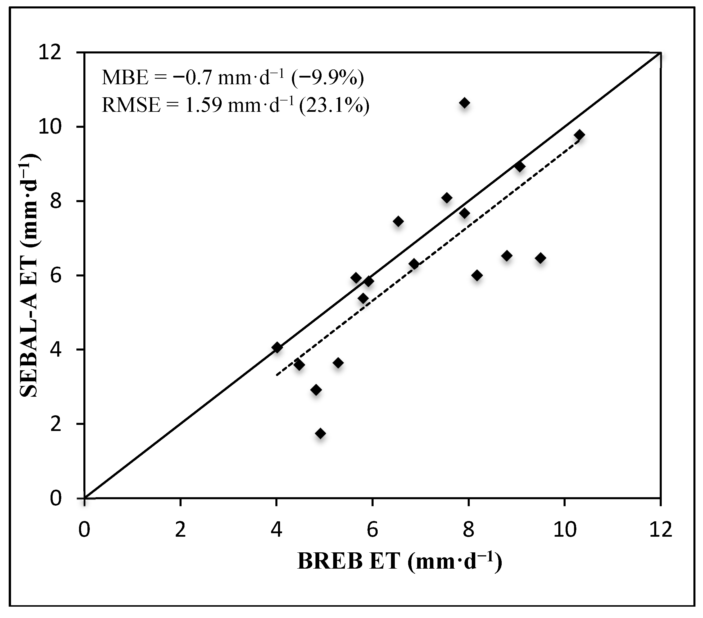
Results from SEBAL-A estimations were compared with BREB results for corn (i.e., both fully irrigated and with limited irrigation) and the comparison is shown in Table 2. The table includes the ET values and corresponding instantaneous evaporative fraction as obtained from SEBAL-A processed images, as well as heights of the corn plants. Figure 1, which includes all corn data (i.e., full and limited irrigation), shows that there was more error incurred when estimating ET when the crops were at early stages of growth. The statistics for all corn data were MBE of −0.7 mm·d⁻¹ (−9.9%), RMSE of 1.59 mm·d⁻¹ (23.1%) and NSCE of 0.24. These indicated that the model was appropriate for ET estimation. This shows an improvement when compared to the original SEBAL model (Figure 2).

In most cases there was an underestimation of ET for smaller EF values (mostly for EF<0.8). Table 2 shows the ET estimation using SEBAL-A on 18 June 2012, when the field was fully irrigated, the corn was 0.31 m tall, and had EF_inst of 0.3. The ET error when compared to BREB was −3.2 mm·d⁻¹ (−64.2%), which was the largest underestimation observed. Other examples were on 30 June 2010 and 16 July 2010, when the EF_inst was 0.69 and 0.78, respectively. For these cases, the ET errors were −3.0 mm·d⁻¹ (−31.7%) and −2.3 mm·d⁻¹ (−25.6%), respectively.

Figure 1. SEBAL-A crop ET compared to measured-ET for corn (from limited and fully irrigated fields).

Figure 1. SEBAL-A crop ET compared to measured-ET for corn (from limited and fully irrigated fields).

Figure 2. Original SEBAL crop ET compared to measured-ET for corn (from limited and fully irrigated fields).

Figure 2. Original SEBAL crop ET compared to measured-ET for corn (from limited and fully irrigated fields).

Table 2. Comparison of SEBAL-A estimated corn ET with BREB ET measured at the USDA ARS LIRF site.

Date	Irrigation Regime *	Crop Height (m)	EF	BREB ET (mm)	SEBAL-A ET (mm)	% Error
24-Jun-08	F	0.25	0.51	5.3	6.1	15
10-Jul-08	F	0.51	0.86	8.2	6.0	−26
11-Aug-08	F	2.29	0.96	5.9	5.8	−1
27-Aug-08	F	2.29	0.98	4.0	4.1	2
2-Jul-08	F	0.36	0.65	4.5	3.6	−19
18-Jul-08	F	1.02	0.91	7.9	9.5	20
30-Jun-10	F	0.80	0.69	9.5	6.5	−32
16-Jul-10	F	1.90	0.78	8.8	6.5	−26
17-Aug-10	F	2.60	0.96	5.8	5.4	−7
24-Jul-10	F	2.10	0.97	7.5	8.1	7
18-Jun-12	F	0.31	0.30	4.9	1.8	−64
18-Jun-12	L	0.47	0.44	4.8	2.9	−39
13-Jul-12	F	1.50	0.97	9.1	8.9	−1
13-Jul-12	L	1.51	0.94	7.9	7.7	−3
20-Jul-12	F	2.12	0.97	10.3	9.8	−5
20-Jul-12	L	1.88	0.87	6.5	7.5	14
5-Aug-12	F	2.60	0.95	6.9	6.3	−8
5-Aug-12	L	2.40	0.90	5.7	5.9	5

* F = full irrigation, L = Limited irrigation.

Table 2. Comparison of SEBAL-A estimated corn ET with BREB ET measured at the USDA ARS LIRF site.

Date	Irrigation Regime *	Crop Height (m)	EF	BREB ET (mm)	SEBAL-A ET (mm)	% Error
24-Jun-08	F	0.25	0.51	5.3	6.1	15
10-Jul-08	F	0.51	0.86	8.2	6.0	−26
11-Aug-08	F	2.29	0.96	5.9	5.8	−1
27-Aug-08	F	2.29	0.98	4.0	4.1	2
2-Jul-08	F	0.36	0.65	4.5	3.6	−19
18-Jul-08	F	1.02	0.91	7.9	9.5	20
30-Jun-10	F	0.80	0.69	9.5	6.5	−32
16-Jul-10	F	1.90	0.78	8.8	6.5	−26
17-Aug-10	F	2.60	0.96	5.8	5.4	−7
24-Jul-10	F	2.10	0.97	7.5	8.1	7
18-Jun-12	F	0.31	0.30	4.9	1.8	−64
18-Jun-12	L	0.47	0.44	4.8	2.9	−39
13-Jul-12	F	1.50	0.97	9.1	8.9	−1
13-Jul-12	L	1.51	0.94	7.9	7.7	−3
20-Jul-12	F	2.12	0.97	10.3	9.8	−5
20-Jul-12	L	1.88	0.87	6.5	7.5	14
5-Aug-12	F	2.60	0.95	6.9	6.3	−8
5-Aug-12	L	2.40	0.90	5.7	5.9	5

* F = full irrigation, L = Limited irrigation.

The errors observed on estimated ET for small EF values were discussed in Part I, and are due to the fact that SEBAL and SEBAL-A are single-source models and, therefore, not fully suitable for heterogeneous surfaces as a result of sparse vegetation cover conditions. The adjustment made on SEBAL was not meant to correct for such errors and, therefore, are still expected to occur. However, it is worth pointing out that some work is being done by other researchers to increase the accuracy of remote sensing models when there is no full cover.

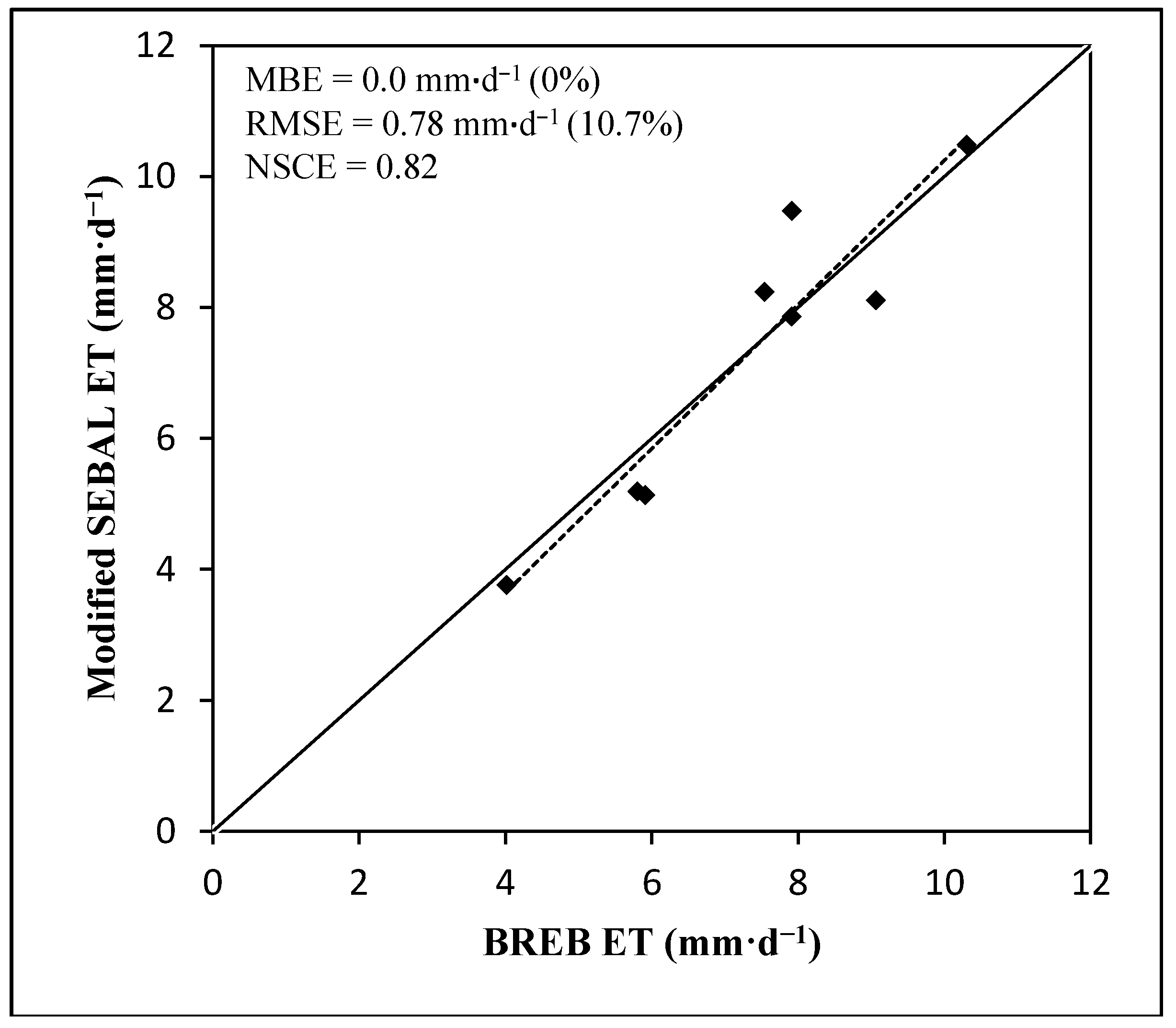
When SEBAL-A was used on only non-stressed irrigated corn fully covering the ground (EF approximately 1), the results were as shown in Figure 3. Most of the points were along the 1:1 line, indicating higher accuracy of the estimated ET when compared to BREB ET. The MBE was 0.0 mm·d⁻¹, which suggests no bias; and RMSE was 0.78 mm·d⁻¹ (10.7%) and the NSCE was 0.82. All ET errors were less than 15% except on 18 July 2008 when the ET was overestimated by 1.6 mm (19.7%). During that day, advective conditions prevailed, with afternoon average wind speeds of 3.3 m s⁻¹, maximum air temperature of 30.7 °C, and minimum air temperature of 14.5 °C.

The overestimation mentioned above may indicate a possible flaw in the model. The stomatal resistance is assumed to be embedded in the EF_inst. In that case, any increase in evaporative demand due to wind and warm air in the afternoon is assumed to have no effect on the stomatal resistance. However, that may not be the case as there seems to be an inverse relationship between canopy moisture conductance and vapor pressure deficit at the canopy surface [2], and different crops may respond differently to the severity of advection. Severe advection may have reduced stomatal conductance, which then resulted in the overestimation of ET by SEBAL-A when compared to BREB ET.

Figure 3. SEBAL-A crop ET compared to measured BREB ET for corn for non-stress full cover corn.

Figure 3. SEBAL-A crop ET compared to measured BREB ET for corn for non-stress full cover corn.

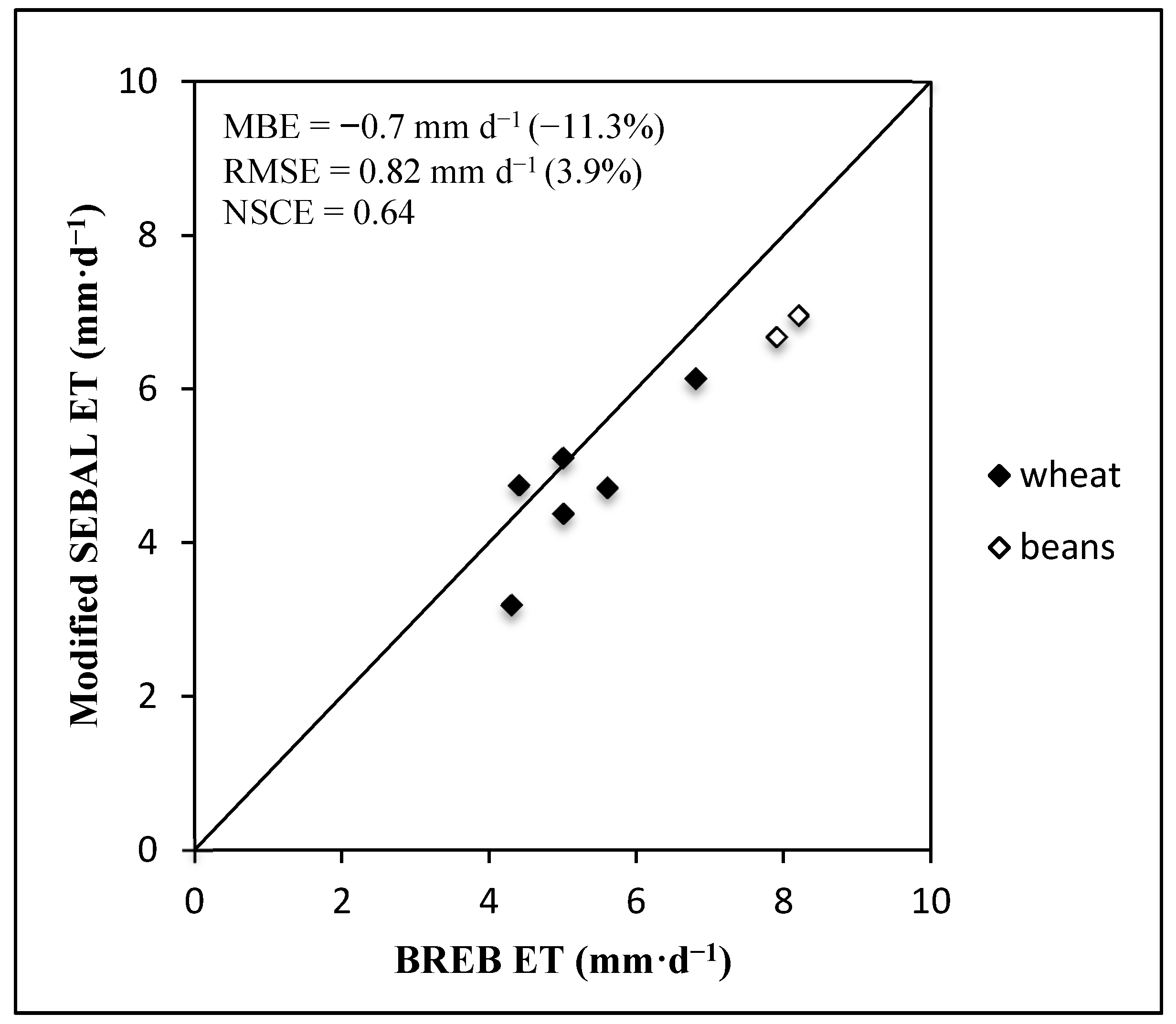
The SEBAL-A model was then used on wheat and beans (Figure 4). Most of the points were below the 1:1 line suggesting that the model slightly underestimated ET for these crops. The MBE was −0.7 mm·d⁻¹ (−11.3%), and the RMSE was 0.82 mm·d⁻¹ (13.9%) and the NSCE was 0.64. While the RMSE was reasonably low at 13.9%, a bias of −11.3% may have a significant impact on the seasonal estimation of ET. In most cases, the beans and wheat had a low EF (i.e., significantly lower than 1), which affects the accuracy as earlier alluded to. However, there were not enough remote sensing images to analyze and conclude on the performance of SEBAL-A model on beans and wheat at various stages of growth. This situation arose because, for the available crop seasons for wheat and beans, the BREB was only installed for a short period; hence, fewer satellite images coincided with the BREB measurement dates.

Figure 4. Comparison of SEBAL-A ET and BREB ET for beans and wheat.

Figure 4. Comparison of SEBAL-A ET and BREB ET for beans and wheat.

The results observed here are comparable to what has been reported in research literature. Generally, researchers report SEBAL errors on daily ET estimation to range between 2% and about 35%. Gowda et al. [25] reported an average accuracy of 85%, while Trezza [26] found the error to range from 2.7% to 35%, with 18.2% being the average error. Singh et al. [9] found that ET_c estimated using SEBAL could be within 5% of measured ET_c. However, he also observed that on certain advective days, SEBAL underestimated ET, pointing out one advective day, where estimated ET_c was 28% lower than measured ET_c. For well-irrigated homogenous surfaces, SEBAL-A, as shown in Figure 3, has its errors random and all but one within 15%, and with MBE of 0 mm·d⁻¹. Errors as high as 10%–20% are tolerable, as long as they are random [3].

The SEBAL-A model, as a single-source model, still has the limitation of not being able to accurately estimate energy heat fluxes on heterogeneous surfaces. Another limitation is that, similar to original SEBAL, the stomatal conductance is embedded in the instantaneous evaporative fraction (EF_inst.). If the stomatal conductance was reduced due to increased atmospheric evaporative demand, as it may happen for some crops on days with severe advection, the model would not be able to account for that, and may then overestimate ET.

4. Conclusions

The modified SEBAL (SEBAL-A) model was tested for transferability on crops and soil moisture conditions different from the standard conditions (i.e., alfalfa crop, 40–60 cm tall and not short of water). The crops evaluated were corn, beans and wheat. When the SEBAL-A model was tested on wheat and beans, there was an average ET underestimation of 11%. This result could have been due to EF values that were significantly below 1, as the crops did not fully cover the ground. The model seems not to perform well under such conditions.

The SEBAL-A model was tested on fully irrigated corn and corn treated to limited irrigation. For the fully irrigated corn, the model performed reasonably well, the MBE was 0.0 mm·d⁻¹, RMSE was 0.78 mm·d⁻¹ (10.7%), and NSCE of 0.82. Since the advection sub-model has a roughness parameter embedded, it can sufficiently estimate advection and, therefore, ET for a range of crop heights. When the model was used on corn with EF significantly less than 1, which included corn at early stages of growth or corn under water stress due to limited irrigation, there were noticeable errors. The largest error observed in this study was 64% when the EF was 0.3. However, it must be noted that these large errors occurred on drier surfaces and early in the growing season when the ET was small.

From the study, it can be concluded that incorporating effective advection in the SEBAL model (SEBAL-A) can improve estimates of ET in semi-arid and arid regions where advection is common. The unique aspect of this model is that it requires basic weather data to achieve accurate estimation of ET. Such weather data consists of daily maximum air temperature (T_max), minimum air temperature (T_min), daily wind run (u) and relative humidity (RH). This is significant as it makes it possible to accurately estimate ET under advective conditions, using remote sensing ET models, even in areas where there are limited weather data, e.g., daily averages.

5. Recommendations

(1)

The modified SEBAL (SEBAL-A) was found to be suitable for use on various crops in arid and semi-arid areas that are well irrigated, fully covering the ground, and are affected by advection. SEBAL-A can be used where there may not be enough weather data to use models such as METRIC.

(2)

Further research should be pursued to evaluate the appropriateness of applying the evaporative fraction (EF) on the advection component in the modified ET₂₄ sub-model.

(3)

As some research is being done to improve the performance of remote sensing models when there is no full cover, such improvements should also be incorporated in this modified version of SEBAL.