
Detection and Delineation of Localized Flooding from WorldView-2 Multispectral Data


Abstract
:
1. Introduction
2. Materials and Methods
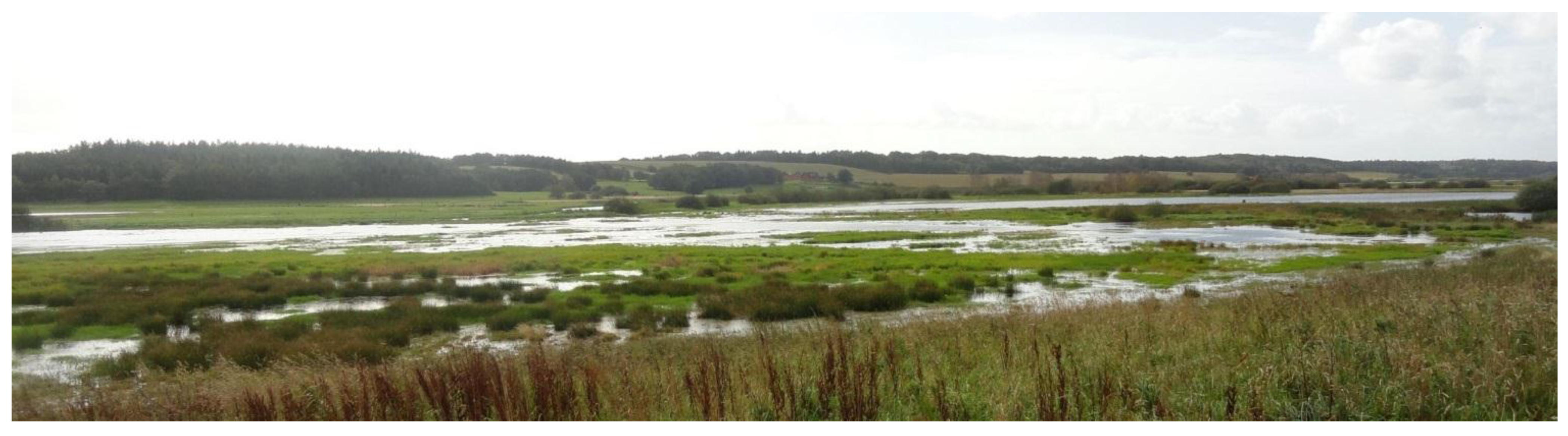
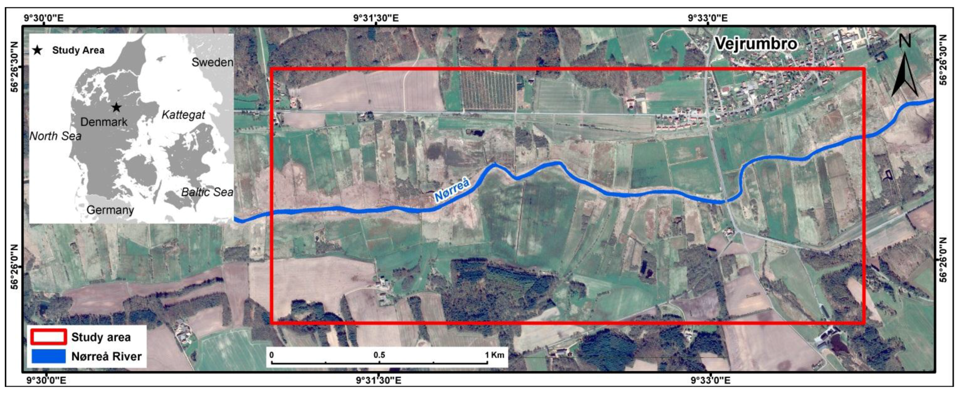
2.1. Study Area

2.2. Remote Sensing Data

| Band | Ground Sample Distance (GSD) (m) | Spectral Range (nm) |
|---|---|---|
| Panchromatic (PAN) | 0.5 | 447–808 |
| Coastal Blue | 2 | 396–458 |
| Blue | 2 | 442–515 |
| Green | 2 | 506–586 |
| Yellow | 2 | 584–632 |
| Red | 2 | 624–694 |
| Red Edge | 2 | 699–749 |
| Near-infrared 1 (NIR-1) | 2 | 765–901 |
| Near-infrared 2 (NIR-2) | 2 | 856–1043 |

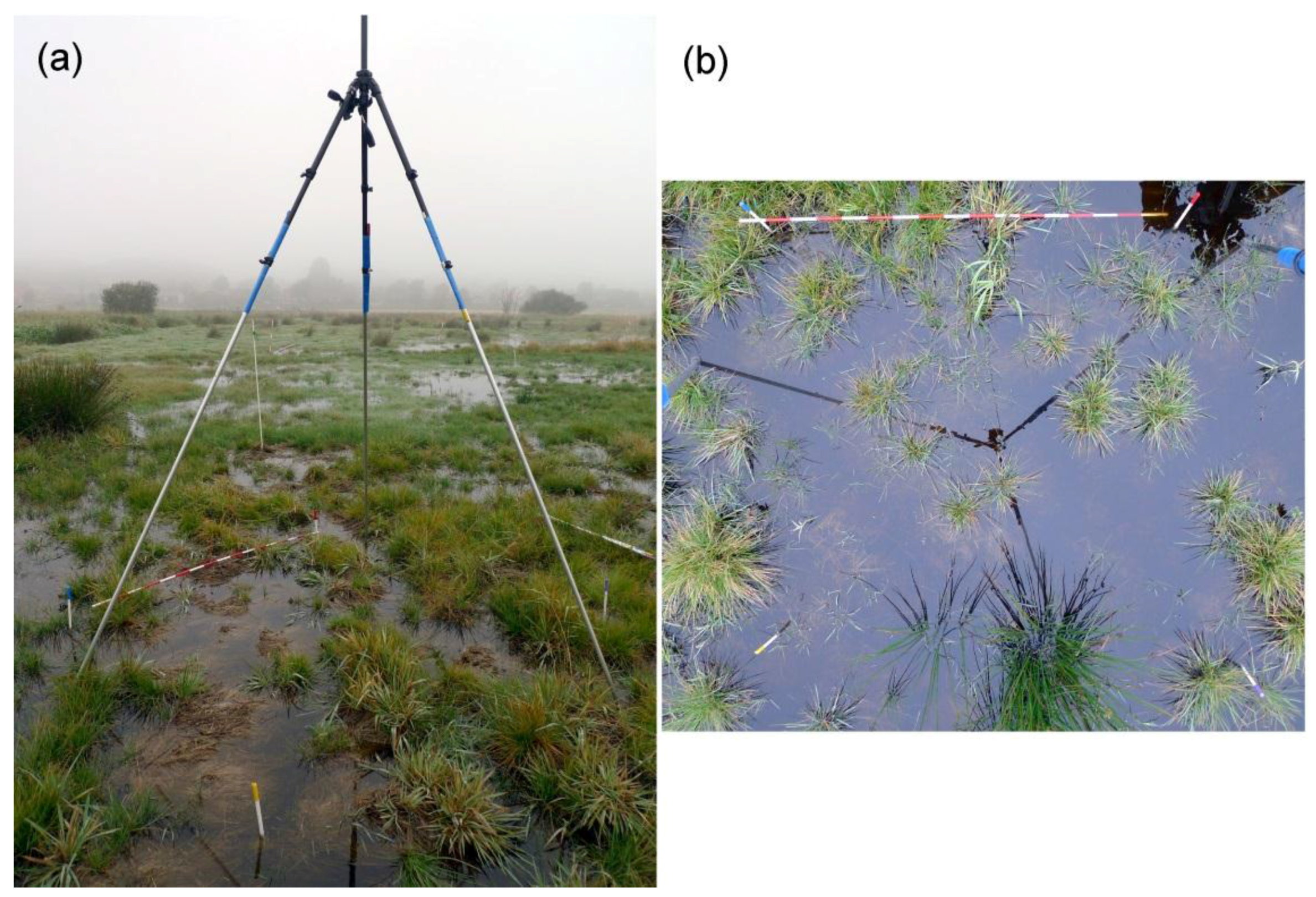
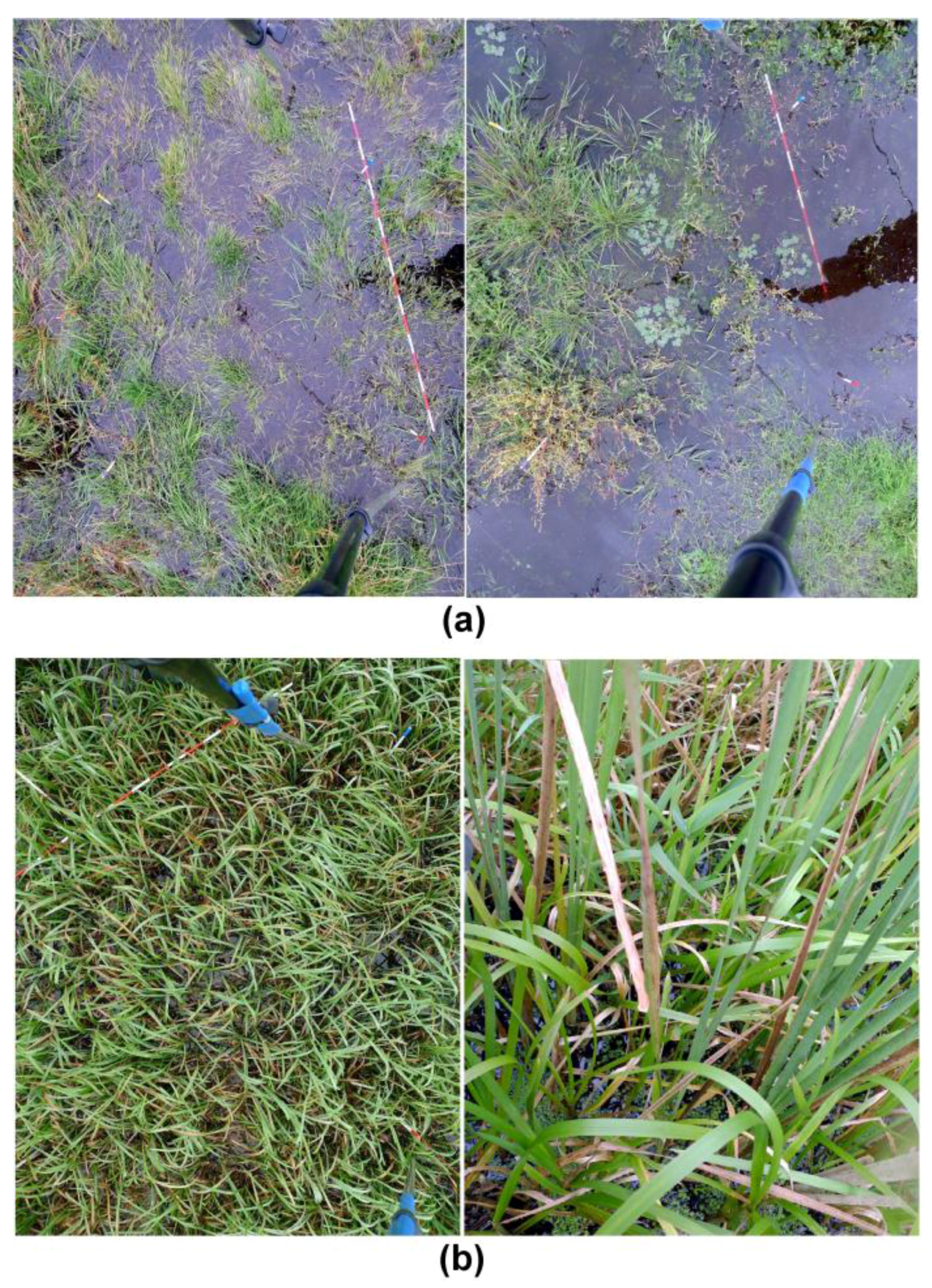
2.3. Field Data Collection
2.4. Image Pre-Processing
2.5. Training Data


2.6. Spectral Indices and Additional Classification Inputs
| Indices | Formula | References |
|---|---|---|
| DVI*—differential vegetation index | NIR – RED | Richardson and Everitt [34] |
| DVW**—difference between vegetation and water | NDVI – NDWI | Gond et al. [35] |
| IFW*—index of free water | NIR – GREEN | Adell and Puech [36] |
| NDWI*—normalized difference water index | (GREEN – NIR)/(GREEN + NIR) | McFeeters [32] |
| NDWI-G—normalized difference water index of Gao | (NIR1 – NIR2)/(NIR1 + NIR2) | Gao [26] |
| NDVI*—normalized difference vegetation index | (NIR – RED)/( NIR + RED) | Tucker [37] |
| OSAVI*—optimized SAVI | (NIR − RED)/(NIR + RED + 0.16) | Rondeaux et al. [38] |
| SAVI*—soil adjusted vegetation index | 1.5 (NIR − RED)/(NIR + RED + 0.5) | Huete [39] |
| SR*—simple ratio | RED/NIR | Pearson and Miller [40] |
| WI*—water index | NIR2/BLUE | Davranche et al. [13] |
| WII*—water impoundment index | NIR2/RED | Caillaud et al. [41] |
| VI*—vegetation index | NIR/RED | Lillesand and Kiefer [42] |
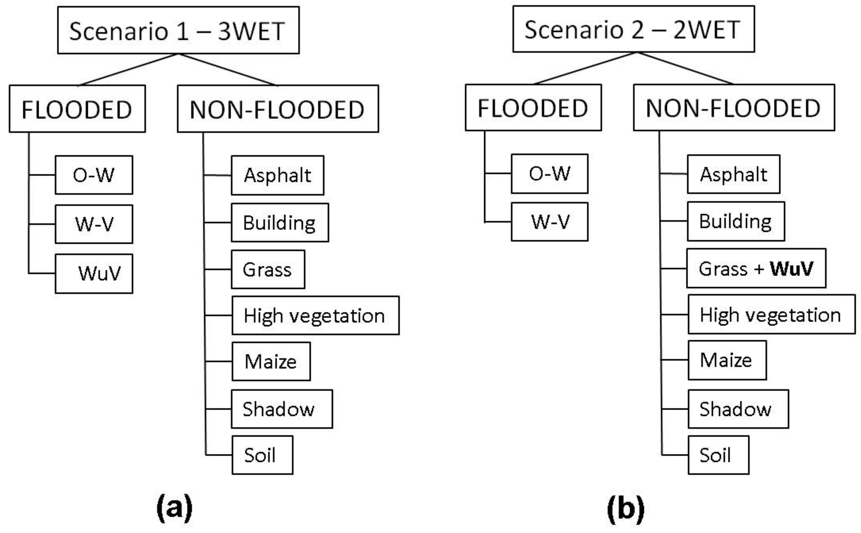
2.7. Classification
| Method # | Analysis Approach | Data Used | Pre-Classification of High Vegetation and Shadows | Training Data | |||
|---|---|---|---|---|---|---|---|
| WV2 Spectral Bands | Spectral Indices | PCA | DTM and SLOPE Raster | ||||
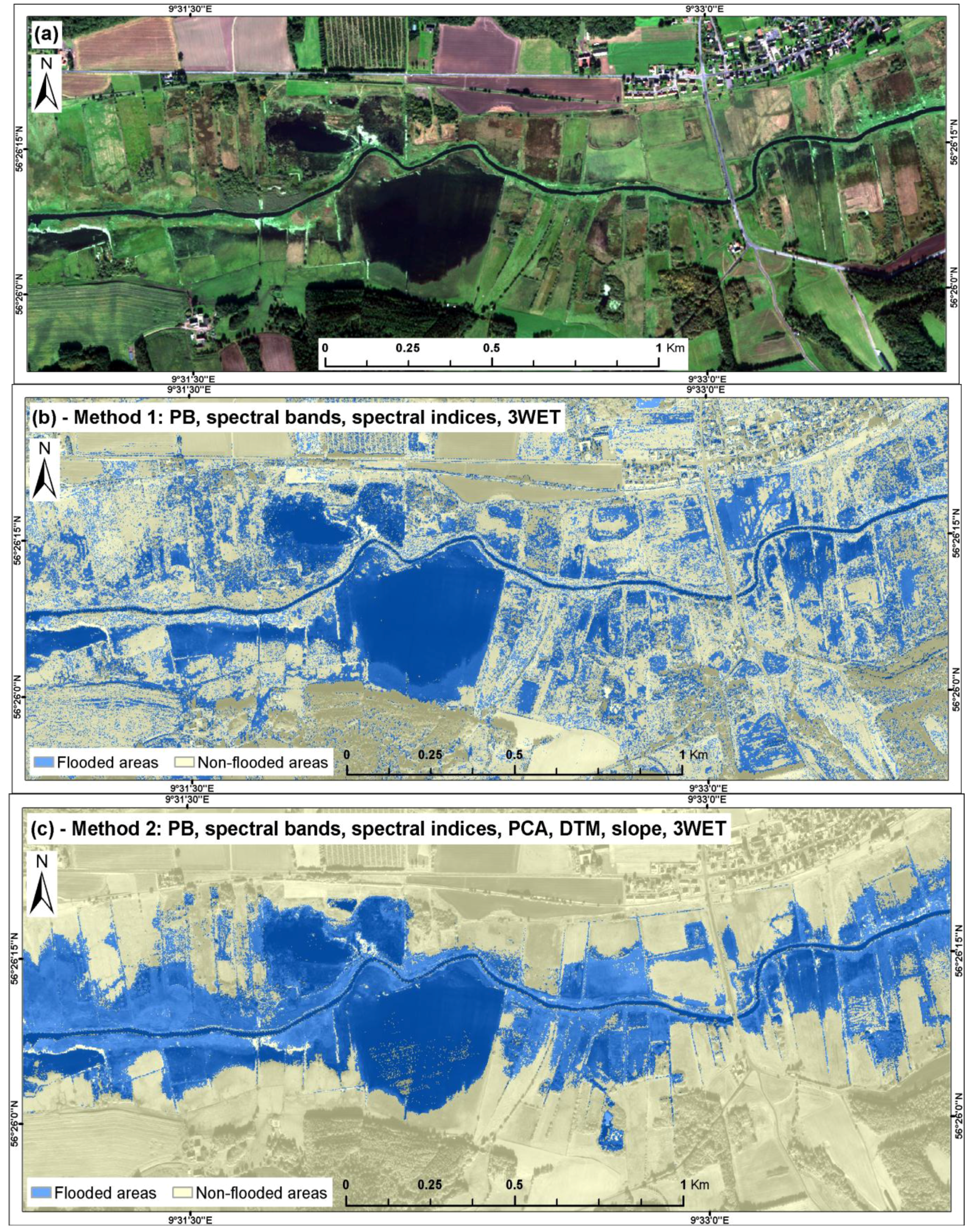
| Method 1 | PB | + | + | 3WET | |||
| Method 2 | PB | + | + | + | + | 3WET | |
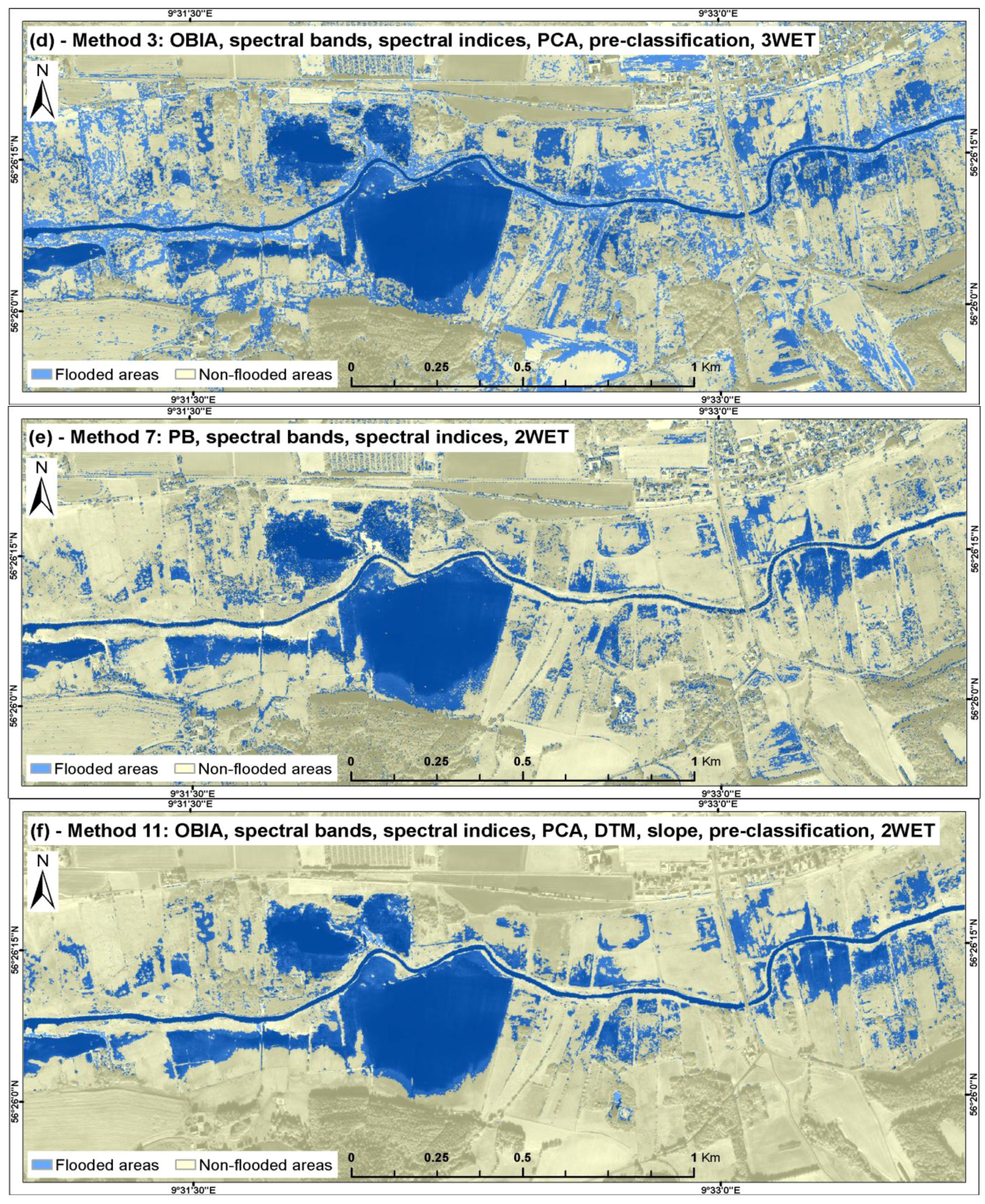
| Method 3 | OBIA | + | + | + | + | 3WET | |
| Method 4 | OBIA | + | + | + | 3WET | ||
| Method 5 | OBIA | + | + | + | + | + | 3WET |
| Method 6 | OBIA | + | + | + | + | 3WET | |
| Method 7 | PB | + | + | 2WET | |||
| Method 8 | PB | + | + | + | + | 2WET | |
| Method 9 | OBIA | + | + | + | + | 2WET | |
| Method 10 | OBIA | + | + | + | 2WET | ||
| Method 11 | OBIA | + | + | + | + | + | 2WET |
| Method 12 | OBIA | + | + | + | + | 2WET | |
2.8. Accuracy Assessment
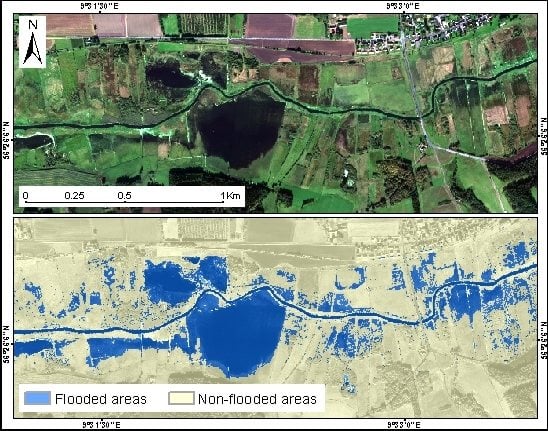
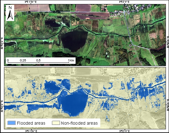
3. Results
| Method # | Reference Data | Total | OA (%) | Flooded Class | QD (%) | AD (%) | ||||
|---|---|---|---|---|---|---|---|---|---|---|
| F | N-F | Comp. (%) | Corr. (%) | |||||||
| 1 | Classification data | F | 107 | 41 | 148 | 77 | 79 | 72 | 4.3 | 18.7 |
| N-F | 28 | 124 | 152 | |||||||
| Total | 135 | 165 | 300 | |||||||
| 2 | Classification data | F | 123 | 17 | 140 | 90 | 91 | 88 | 1.7 | 8.0 |
| N-F | 12 | 148 | 160 | |||||||
| Total | 135 | 165 | 300 | |||||||
| 3 | Classification data | F | 114 | 29 | 143 | 83 | 84 | 80 | 2.7 | 14.0 |
| N-F | 21 | 136 | 157 | |||||||
| Total | 135 | 165 | 300 | |||||||
| 4 | Classification data | F | 110 | 33 | 143 | 81 | 81 | 77 | 2.7 | 16.7 |
| N-F | 25 | 132 | 157 | |||||||
| Total | 135 | 165 | 300 | |||||||
| 5 | Classification data | F | 127 | 16 | 143 | 92 | 94 | 89 | 2.7 | 5.3 |
| N-F | 8 | 149 | 157 | |||||||
| Total | 135 | 165 | 300 | |||||||
| 6 | Classification data | F | 127 | 19 | 146 | 91 | 94 | 87 | 3.7 | 5.3 |
| N-F | 8 | 146 | 154 | |||||||
| Total | 135 | 165 | 300 | |||||||
| 7 | Classification data | F | 97 | 24 | 121 | 88 | 88 | 80 | 3.7 | 8.7 |
| N-F | 13 | 166 | 179 | |||||||
| Total | 110 | 190 | 300 | |||||||
| 8 | Classification data | F | 97 | 18 | 115 | 90 | 88 | 84 | 1.7 | 8.7 |
| N-F | 13 | 172 | 185 | |||||||
| Total | 110 | 190 | 300 | |||||||
| 9 | Classification data | F | 94 | 6 | 100 | 93 | 85 | 94 | 3.3 | 4.0 |
| N-F | 16 | 184 | 200 | |||||||
| Total | 110 | 190 | 300 | |||||||
| 10 | Classification data | F | 91 | 18 | 109 | 88 | 83 | 83 | 0.3 | 12.0 |
| N-F | 19 | 172 | 191 | |||||||
| Total | 110 | 190 | 300 | |||||||
| 11 | Classification data | F | 100 | 5 | 105 | 95 | 91 | 95 | 1.7 | 3.3 |
| N-F | 10 | 185 | 195 | |||||||
| Total | 110 | 190 | 300 | |||||||
| 12 | Classification data | F | 97 | 7 | 104 | 93 | 88 | 93 | 2.0 | 4.7 |
| N-F | 13 | 183 | 196 | |||||||
| Total | 110 | 190 | 300 | |||||||


4. Discussion
4.1. Major Misclassification Issues
4.2. Application of SWIR Data
4.3. Application of Topographic Data
5. Conclusions
Acknowledgments
Author Contributions
Conflicts of Interest
References
- Chignell, S.; Anderson, R.; Evangelista, P.; Laituri, M.; Merritt, D. Multi-temporal independent component analysis and Landsat 8 for delineating maximum extent of the 2013 Colorado front range flood. Remote Sens. 2015, 7, 9822–9843. [Google Scholar] [CrossRef]
- Pierdicca, N.; Pulvirenti, L.; Chini, M.; Guerriero, L.; Candela, L. Observing floods from space: Experience gained from COSMO-SkyMed observations. Acta Astronaut. 2013, 84, 122–133. [Google Scholar] [CrossRef]
- Thomas, R.F.; Kingsford, R.T.; Lu, Y.; Hunter, S.J. Landsat mapping of annual inundation (1979–2006) of the Macquarie Marshes in semi-arid Australia. Int. J. Remote Sens. 2011, 32, 4545–4569. [Google Scholar] [CrossRef]
- Smith, L.C. Satellite remote sensing of river inundation area, stage, and discharge: A review. Hydrol. Process. 1997, 11, 1427–1439. [Google Scholar] [CrossRef]
- Ward, D.P.; Petty, A.; Setterfield, S.A.; Douglas, M.M.; Ferdinands, K.; Hamilton, S.K.; Phinn, S. Floodplain inundation and vegetation dynamics in the Alligator Rivers region (Kakadu) of northern Australia assessed using optical and radar remote sensing. Remote Sens. Environ. 2014, 147, 43–55. [Google Scholar] [CrossRef]
- Jensen, J.R. Remote Sensing of the Environment: An Earth Resource Perspective., 2nd ed.; Pearson Prentice Hall: Upper Saddle River, NJ, USA, 2007; p. 592. [Google Scholar]
- Lillesand, T.M.; Kiefer, R.W.; Chipman, J.W. Remote Sensing and Image Interpretation, 6th ed.; John Wiley & Sons: Hoboken, NJ, USA.
- Silva, T.F.; Costa, M.F.; Melack, J.; Novo, E.L.M. Remote sensing of aquatic vegetation: Theory and applications. Environ. Monit. Assess. 2008, 140, 131–145. [Google Scholar] [CrossRef] [PubMed]
- European Communities (EC). Directive 2007/60/EC of the European Parliament and of the Council of 23 October 2007 on the assessment and management of flood risks. Off. J. European Communities 2007, 1, L288/27. [Google Scholar]
- European Communities (EC). COUNCIL REGULATION (EC) No 73/2009 of 19 January 2009 establishing common rules for direct support schemes for farmers under the common agricultural policy and establishing certain support schemes for farmers, amending Regulations (EC) No 1290/2005, (EC) No 247/2006, (EC) No 378/2007 and repealing Regulation (EC) No 1782/2003. Off. J. European Communities 2009, L 30, 16–19. [Google Scholar]
- Jones, K.; Lanthier, Y.; van der Voet, P.; van Valkengoed, E.; Taylor, D.; Fernández-Prieto, D. Monitoring and assessment of wetlands using Earth Observation: The GlobWetland project. J. Environ. Manage. 2009, 90, 2154–2169. [Google Scholar] [CrossRef] [PubMed]
- Matthews, G.V.T. The Ramsar Convention on Wetlands: Its History and Development; Ramsar Convention Bureau: Gland, Switzerland, 1993. [Google Scholar]
- Davranche, A.; Poulin, B.; Lefebvre, G. Mapping flooding regimes in Camargue wetlands using seasonal multispectral data. Remote Sens. Environ. 2013, 138, 165–171. [Google Scholar] [CrossRef]
- Davranche, A.; Lefebvre, G.; Poulin, B. Wetland monitoring using classification trees and SPOT-5 seasonal time series. Remote Sens. Environ. 2010, 114, 552–562. [Google Scholar] [CrossRef]
- Huang, C.; Peng, Y.; Lang, M.; Yeo, I.-Y.; McCarty, G. Wetland inundation mapping and change monitoring using Landsat and airborne LiDAR data. Remote Sens. Environ. 2014, 141, 231–242. [Google Scholar] [CrossRef]
- Zhao, X.; Stein, A.; Chen, X.-L. Monitoring the dynamics of wetland inundation by random sets on multi-temporal images. Remote Sens. Environ. 2011, 115, 2390–2401. [Google Scholar] [CrossRef]
- Klemas, V. Using remote sensing to select and monitor wetland restoration sites: An overview. J. Coast. Res. 2013, 29, 958–970. [Google Scholar] [CrossRef]
- Ozesmi, S.L.; Bauer, M.E. Satellite remote sensing of wetlands. Wetl. Ecol. Manag. 2002, 10, 381–402. [Google Scholar] [CrossRef]
- Mallinis, G.; Gitas, I.Z.; Giannakopoulos, V.; Maris, F.; Tsakiri-Strati, M. An object-based approach for flood area delineation in a transboundary area using ENVISAT ASAR and LANDSAT TM data. Int. J. Digit. Earth 2013, 6, 124–136. [Google Scholar] [CrossRef]
- Robertson, L.D.; Douglas, J.K.; Davies, C. Spatial analysis of wetlands at multiple scales in Eastern Ontario using remote sensing and GIS. In Proceedings of 32nd Canadian Symposium on Remote Sensing, Sherbrooke, QC, Canada, 13–16 June 2011.
- Schumann, G.J.P.; Neal, J.C.; Mason, D.C.; Bates, P.D. The accuracy of sequential aerial photography and SAR data for observing urban flood dynamics, a case study of the UK summer 2007 floods. Remote Sens. Environ. 2011, 115, 2536–2546. [Google Scholar] [CrossRef]
- Frazier, P.S.; Page, K.J. Water body detection and delineation with Landsat TM data. Photogramm. Eng. Remote Sens. 2000, 66, 1461–1467. [Google Scholar]
- Feyisa, G.L.; Meilby, H.; Fensholt, R.; Proud, S.R. Automated Water Extraction Index: A new technique for surface water mapping using Landsat imagery. Remote Sens. Environ. 2014, 140, 23–35. [Google Scholar] [CrossRef]
- Li, W.; Du, Z.; Ling, F.; Zhou, D.; Wang, H.; Gui, Y.; Sun, B.; Zhang, X. A Comparison of land surface water mapping using the normalized difference water index from TM, ETM+ and ALI. Remote Sens. 2013, 5, 5530–5549. [Google Scholar] [CrossRef]
- Xu, H.Q. Modification of normalised difference water index (NDWI) to enhance open water features in remotely sensed imagery. Int. J. Remote Sens. 2006, 27, 3025–3033. [Google Scholar] [CrossRef]
- Gao, B.-C. NDWI—A normalized difference water index for remote sensing of vegetation liquid water from space. Remote Sens. Environ. 1996, 58, 257–266. [Google Scholar] [CrossRef]
- Tucker, C.J. Remote sensing of leaf water content in the near infrared. Remote Sens. Environ. 1980, 10, 23–32. [Google Scholar] [CrossRef]
- DigitalGlobe. DigitalGlobe Core Imagery Product Guide; DigitalGlobe Inc.: Longmont, CO, USA, 2014. [Google Scholar]
- KMS. Produktspecification. Danmarks Højdemodel, DHM/Terræn. Data Version 1.0; National Survey and Cadastre: Copenhagen, Denamrk, 2012. [Google Scholar]
- Richter, R.; Schläpfer, D. Atmospheric/Topographic Correction for Satellite Imagery; DLR: Wessling, Germany, 2014. [Google Scholar]
- Davis, S.M.; Landgrebe, D.A.; Phillips, T.L.; Swain, P.H.; Hoffer, R.M.; Lindenlaub, J.C.; Silva, L.F. Remote Sensing: The Quantitative Approach; McGraw-Hill International Book Co.: New York, NY, USA, 1978. [Google Scholar]
- McFeeters, S.K. The use of the Normalized Difference Water Index (NDWI) in the delineation of open water features. Int. J. Remote Sens. 1996, 17, 1425–1432. [Google Scholar] [CrossRef]
- Updike, T.; Comp, C. Radiometric Use of WorldView-2 Imagery; Digital Globe Inc.: Longmont, CO, USA, 2010; pp. 1–17. [Google Scholar]
- Richardson, A.J.; Everitt, J.H. Using spectral vegetation indices to estimate rangeland productivity. Geocarto Int. 1992, 7, 63–69. [Google Scholar] [CrossRef]
- Gond, V.; Bartholomé, E.; Ouattara, F.; Nonguierma, A.; Bado, L. Surveillance et cartographie des plans d’eau et des zones humides et inondables en régions arides avec l’instrument VEGETATION embarqué sur SPOT-4. Int. J. Remote Sens. 2004, 25, 987–1004. [Google Scholar] [CrossRef]
- Adell, C.; Puech, C. Will the spatial analysis of water maps extracted by remote satellite detection allow locating the footprints of hunting activity in the Camargue? Bull. Soc. Fr. Photogramm. Teledetec. 2003, 76–86. [Google Scholar]
- Tucker, C.J. Red and photographic infrared linear combinations for monitoring vegetation. Remote Sens. Environ. 1979, 8, 127–150. [Google Scholar] [CrossRef]
- Rondeaux, G.; Steven, M.; Baret, F. Optimization of soil-adjusted vegetation indices. Remote Sens. Environ. 1996, 55, 95–107. [Google Scholar] [CrossRef]
- Huete, A.R. A soil-adjusted vegetation index (SAVI). Remote Sens. Environ. 1988, 25, 295–309. [Google Scholar] [CrossRef]
- Pearson, R.L.; Miller, L.D. Remote mapping of standing crop biomass for estimation of the productivity of the short-grass Prairie, Pawnee National Grasslands, Colorado. In Proceedings of the Eighth International Symposium on Remote Sensing of Environment, Ann Arbor, MI, USA, 2–6 October 1972; pp. 1357–1381.
- Caillaud, L.; Guillaumont, B.; Manaud, F. Essai de discrimination des modes d’utilisation des marais maritimes par analyse multitemporelle d’images SPOT, application aux marais maritimes du Centre Ouest; IFREMER: Brest, France, 1991; p. 45. [Google Scholar]
- Lillesand, T.M.; Kiefer, R.W. Remote Sensing and Image Interpretation, 2nd ed.; John Wiley and Sons: New York, NY, USA, 1987. [Google Scholar]
- Friedl, M.A.; Brodley, C.E. Decision tree classification of land cover from remotely sensed data. Remote Sens. Environ. 1997, 61, 399–409. [Google Scholar] [CrossRef]
- Breiman, L.; Friedman, J.; Stone, C.J.; Olshen, R.A. Classification and Regression Trees; Wadsworth International Group: Belmont, CA, USA, 1984. [Google Scholar]
- Trimble. eCognition Developer 9.0 - Reference Book; Trimble Germany GmbH: Munich, Germany, 2014. [Google Scholar]
- Blaschke, T. Object based image analysis for remote sensing. ISPRS J. Photogramm. Remote Sens. 2010, 65, 2–16. [Google Scholar] [CrossRef]
- Blaschke, T.; Hay, G.J.; Kelly, M.; Lang, S.; Hofmann, P.; Addink, E.; Queiroz Feitosa, R.; van der Meer, F.; van der Werff, H.; van Coillie, F.; et al. Geographic Object-Based Image Analysis—Towards a new paradigm. ISPRS J. Photogramm. Remote Sens. 2014, 87, 180–191. [Google Scholar] [CrossRef] [PubMed]
- Blaschke, T.; Strobl, J. What’s wrong with pixels? Some recent developments interfacing remote sensing and GIS. Was ist mit den Pixeln los? Neue Entwicklungen zur Integration von Fernerkundung und GIS 2001, 14, 12–17. [Google Scholar]
- Baatz, M.; Schäpe, A. Multiresolution segmentation: an optimization approach for high quality multi-scale image segmentation. Angew. Geogr. Inf. 2000, 12, 12–23. [Google Scholar]
- Laben, C.A.; Brower, B.V. Process for enhancing the spatial resolution of multispectral imagery using pan-sharpening. U.S. Patent No. 6,011,875, 4 January 2000. [Google Scholar]
- Herrera-Cruz, V.; Koudogbo, F.; Herrera, V. TerraSAR-X Rapid Mapping for Flood Events. In Proceedings of the International Society for Photogrammetry and Remote Sensing (Earth Imaging for Geospatial Information), Hannover, Germany, 2009; pp. 170–175.
- Jain, S.K.; Singh, R.D.; Jain, M.K.; Lohani, A.K. Delineation of flood-prone areas using remote sensing techniques. Water Resour. Manag. 2005, 19, 333–347. [Google Scholar] [CrossRef]
- Lu, S.L.; Wu, B.F.; Yan, N.N.; Wang, H. Water body mapping method with HJ-1A/B satellite imagery. Int. J. Appl. Earth Obs. 2011, 13, 428–434. [Google Scholar] [CrossRef]
- ERDAS. IMAGINE Subpixel Classifier User’s Guide; ERDAS, Inc.: Norcross, GA, USA, 2009. [Google Scholar]
- Pontius, R.G.; Millones, M. Death to Kappa: Birth of quantity disagreement and allocation disagreement for accuracy assessment. Int. J. Remote Sens. 2011, 32, 4407–4429. [Google Scholar] [CrossRef]
- Pontius, R.G.; Santacruz, A. Quantity, exchange, and shift components of difference in a square contingency table. Int. J. Remote Sens. 2014, 35, 7543–7554. [Google Scholar] [CrossRef]
- Arroyo, L.A.; Johansen, K.; Armston, J.; Phinn, S. Integration of LiDAR and QuickBird imagery for mapping riparian biophysical parameters and land cover types in Australian tropical savannas. For. Ecol. Manag. 2010, 259, 598–606. [Google Scholar] [CrossRef]
- Grenier, M.; Demers, A.M.; Labrecque, S.; Benoit, M.; Fournier, R.A.; Drolet, B. An object-based method to map wetland using RADARSAT-1 and Landsat ETM images: Test case on two sites in Quebec, Canada. Can. J. Remote Sens. 2007, 33, S28–S45. [Google Scholar] [CrossRef]
- Byrd, K.B.; O’Connell, J.L.; Di Tommaso, S.; Kelly, M. Evaluation of sensor types and environmental controls on mapping biomass of coastal marsh emergent vegetation. Remote Sens. Environ. 2014, 149, 166–180. [Google Scholar] [CrossRef]
- Beget, M.E.; Di Bella, C.M. Flooding: The effect of water depth on the spectral response of grass canopies. J. Hydrol. 2007, 335, 285–294. [Google Scholar] [CrossRef]
- Jakubauskas, M.; Kindscher, K.; Fraser, A.; Debinski, D.; Price, K.P. Close-range remote sensing of aquatic macrophyte vegetation cover. Int. J. Remote Sens. 2000, 21, 3533–3538. [Google Scholar] [CrossRef]
- Baret, F.; Guyot, G.; Begue, A.; Maurel, P.; Podaire, A. Complementarity of middle-infrared with visible and near-infrared reflectance for monitoring wheat canopies. Remote Sens. Environ. 1988, 26, 213–225. [Google Scholar] [CrossRef]
- Brivio, P.A.; Colombo, R.; Maggi, M.; Tomasoni, R. Integration of remote sensing data and GIS for accurate mapping of flooded areas. Int. J. Remote Sens. 2002, 23, 429–441. [Google Scholar] [CrossRef]
- Pierdicca, N.; Chini, M.; Pulvirenti, L.; Macina, F. Integrating physical and topographic information into a fuzzy scheme to map flooded area by SAR. Sensors 2008, 8, 4151–4164. [Google Scholar] [CrossRef]
- Pulvirenti, L.; Pierdicca, N.; Chini, M.; Guerriero, L. An algorithm for operational flood mapping from Synthetic Aperture Radar (SAR) data using fuzzy logic. Nat. Hazards Earth Syst. Sci. 2011, 11, 529–540. [Google Scholar] [CrossRef]
- Zwenzner, H.; Voigt, S. Improved estimation of flood parameters by combining space based SAR data with very high resolution digital elevation data. Hydrol. Earth Syst. Sci. 2009, 13, 567–576. [Google Scholar] [CrossRef]
© 2015 by the authors; licensee MDPI, Basel, Switzerland. This article is an open access article distributed under the terms and conditions of the Creative Commons Attribution license (http://creativecommons.org/licenses/by/4.0/).
Share and Cite
Malinowski, R.; Groom, G.; Schwanghart, W.; Heckrath, G. Detection and Delineation of Localized Flooding from WorldView-2 Multispectral Data. Remote Sens. 2015, 7, 14853-14875. https://doi.org/10.3390/rs71114853
Malinowski R, Groom G, Schwanghart W, Heckrath G. Detection and Delineation of Localized Flooding from WorldView-2 Multispectral Data. Remote Sensing. 2015; 7(11):14853-14875. https://doi.org/10.3390/rs71114853
Chicago/Turabian StyleMalinowski, Radosław, Geoff Groom, Wolfgang Schwanghart, and Goswin Heckrath. 2015. "Detection and Delineation of Localized Flooding from WorldView-2 Multispectral Data" Remote Sensing 7, no. 11: 14853-14875. https://doi.org/10.3390/rs71114853
APA StyleMalinowski, R., Groom, G., Schwanghart, W., & Heckrath, G. (2015). Detection and Delineation of Localized Flooding from WorldView-2 Multispectral Data. Remote Sensing, 7(11), 14853-14875. https://doi.org/10.3390/rs71114853