
A Remote Sensing Approach to Estimate Vertical Profile Classes of Phytoplankton in a Eutrophic Lake


 ,
,  and
and
Abstract
:
1. Introduction
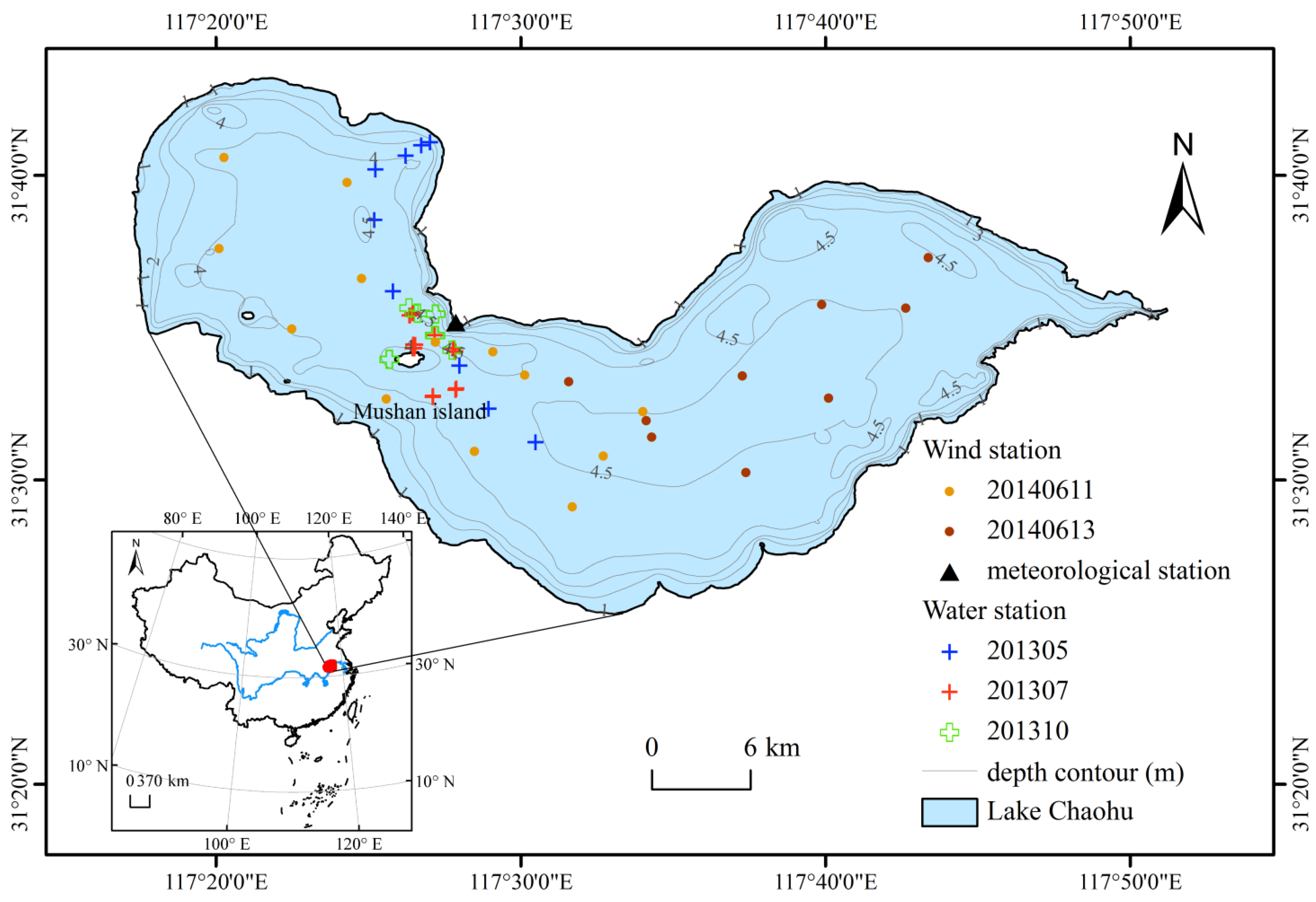
2. Study Region
3. Methods
3.1. Field Measurements
3.2. MODIS Satellite Data
3.3. Parameterization of Vertical Chla Profiles
3.4. Algal Bloom Indexes
3.5. Classification and Regression Tree (CART)
4. Results
4.1. Vertical Characteristics of Optically Active Substances

| Water Surface Value | CV of Vertical Profile | |||||||||
|---|---|---|---|---|---|---|---|---|---|---|
| N | Mean | SD | Min | Max | N | Mean (%) | SD (%) | Min (%) | Max (%) | |
| Chla | 64 | 352.68 | 922.32 | 26.00 | 6988.29 | 64 | 67 | 68 | 4 | 239 |
| SPIM | 64 | 31.33 | 17.47 | 10.00 | 88.00 | 41 | 28 | 14 | 8 | 64 |
| DOC | 64 | 27.27 | 23.21 | 3.23 | 126.32 | 9 | 14 | 9 | 6 | 34 |
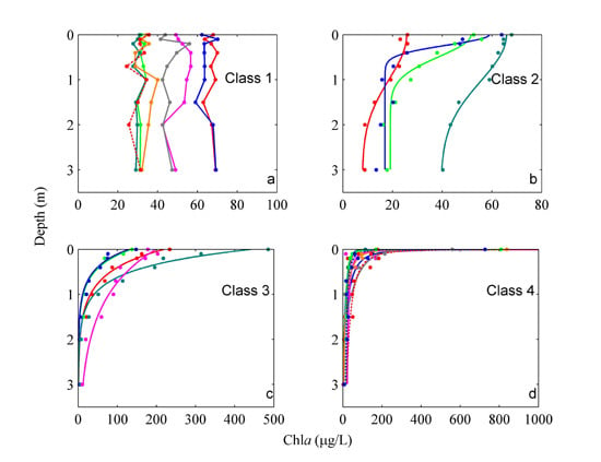
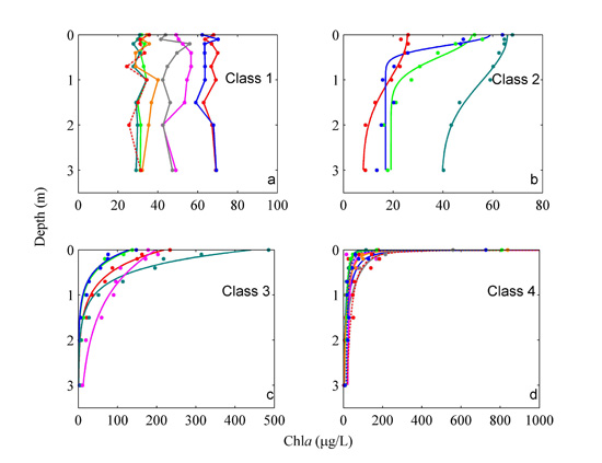
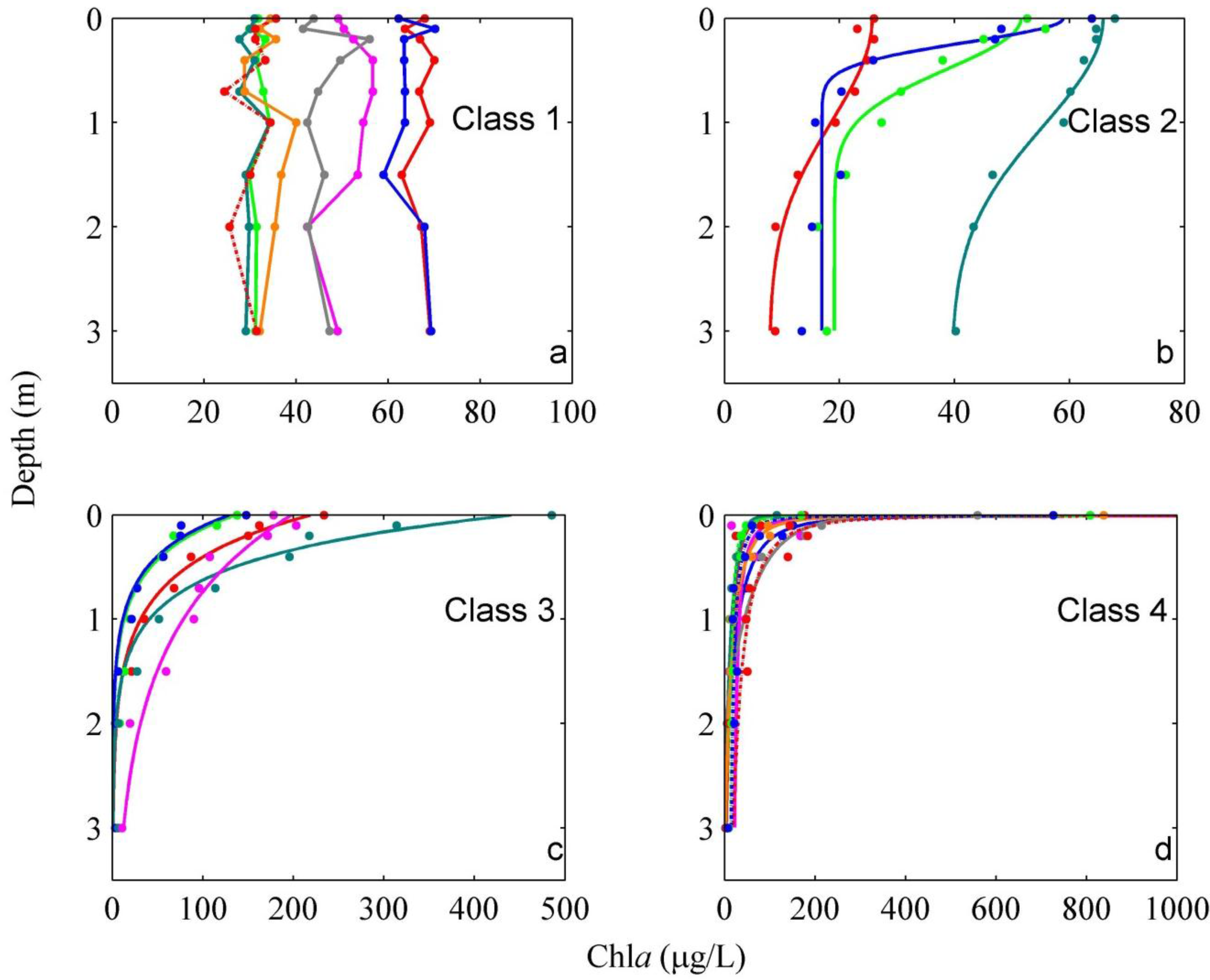
| Class | N | Average CV | Chla Vertical Profile Class | Fitted Function | R2 | RMSE |
|---|---|---|---|---|---|---|
| Class 1 | 27 | 19.53% | uniform | – | 9.57 | |
| Class 2 | 9 | 29.25% | Gaussian | 0.85 | 3.36 | |
| Class 3 | 12 | 97.73% | exponential | 0.91 | 23.29 | |
| Class 4 | 16 | 163.60% | hyperbolic | 0.86 | 20.15 |

| Class | Parameters | Min | Max | Mean | Sd |
|---|---|---|---|---|---|
| Class 2 | C0 | 7.76 | 39.81 | 22.42 | 10.85 |
| σ | 0.02 | 0.41 | 0.20 | 0.15 | |
| h | 1.48 | 75.59 | 34.08 | 26.94 | |
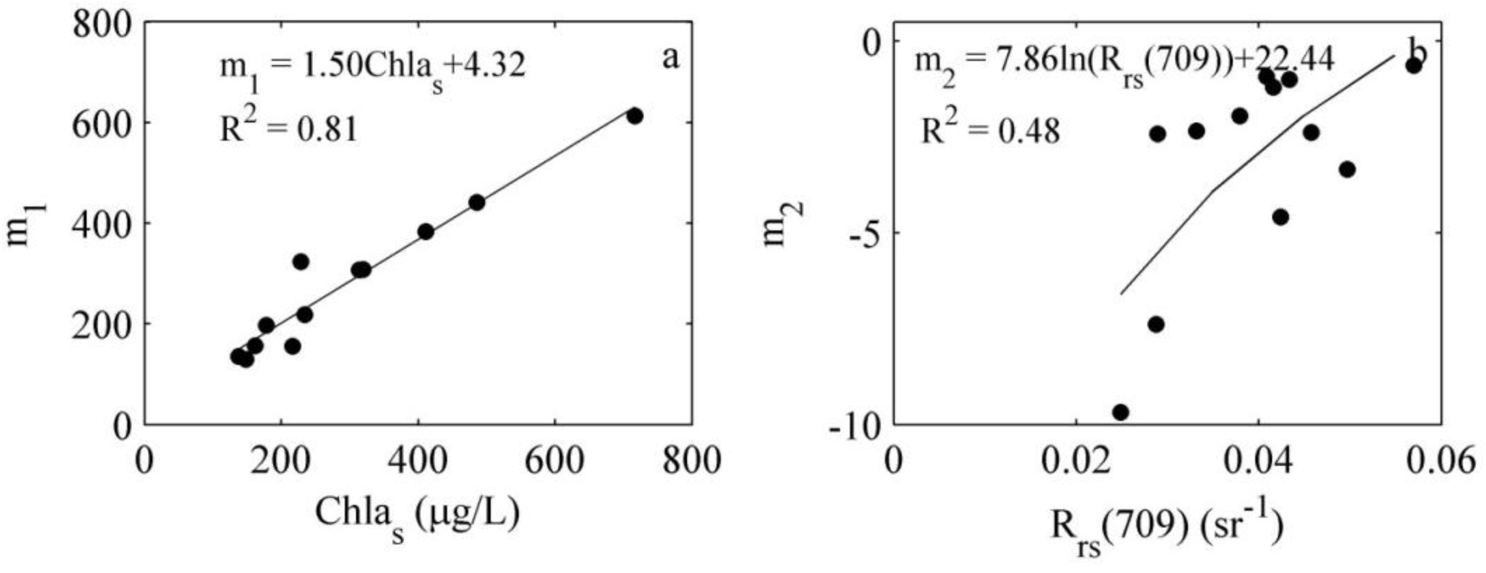
| Class 3 | m1 | 129.4 | 613.30 | 280.98 | 146.54 |
| m2 | −9.67 | −0.64 | −3.15 | 2.79 | |
| Class 4 | n1 | 12.46 | 80.63 | 29.01 | 19.82 |
| n2 | −1.10 | −0.28 | −0.71 | 0.26 |
4.2. Identification of Chla Vertical Profile Classes Using in situ Rrs
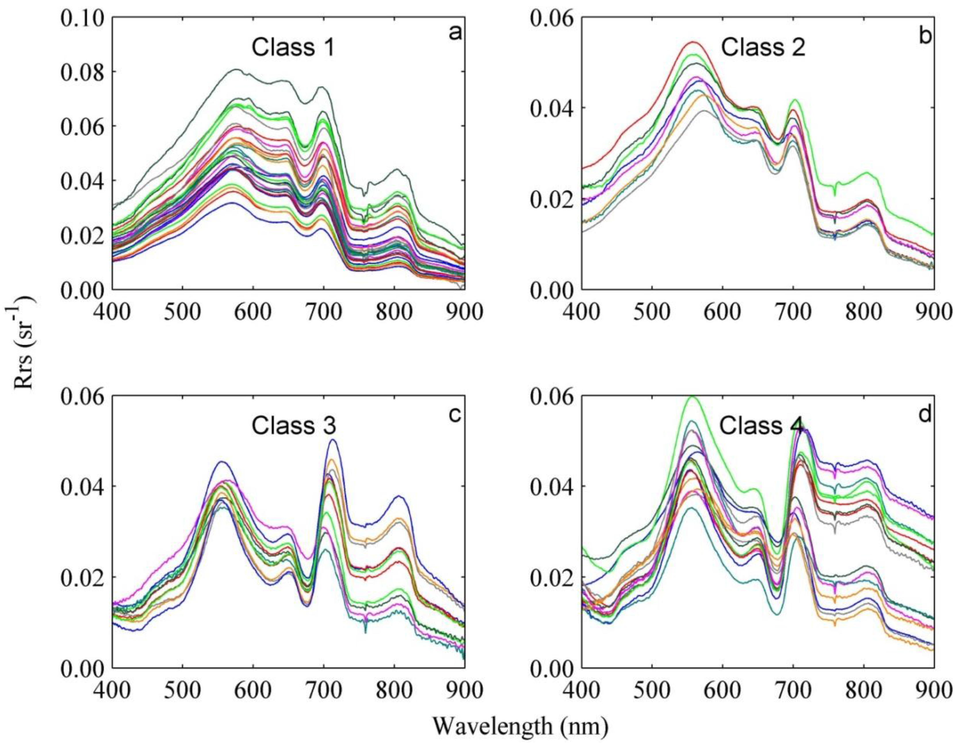
4.2.1. Rrs Response to Algae Vertical Profile Classes
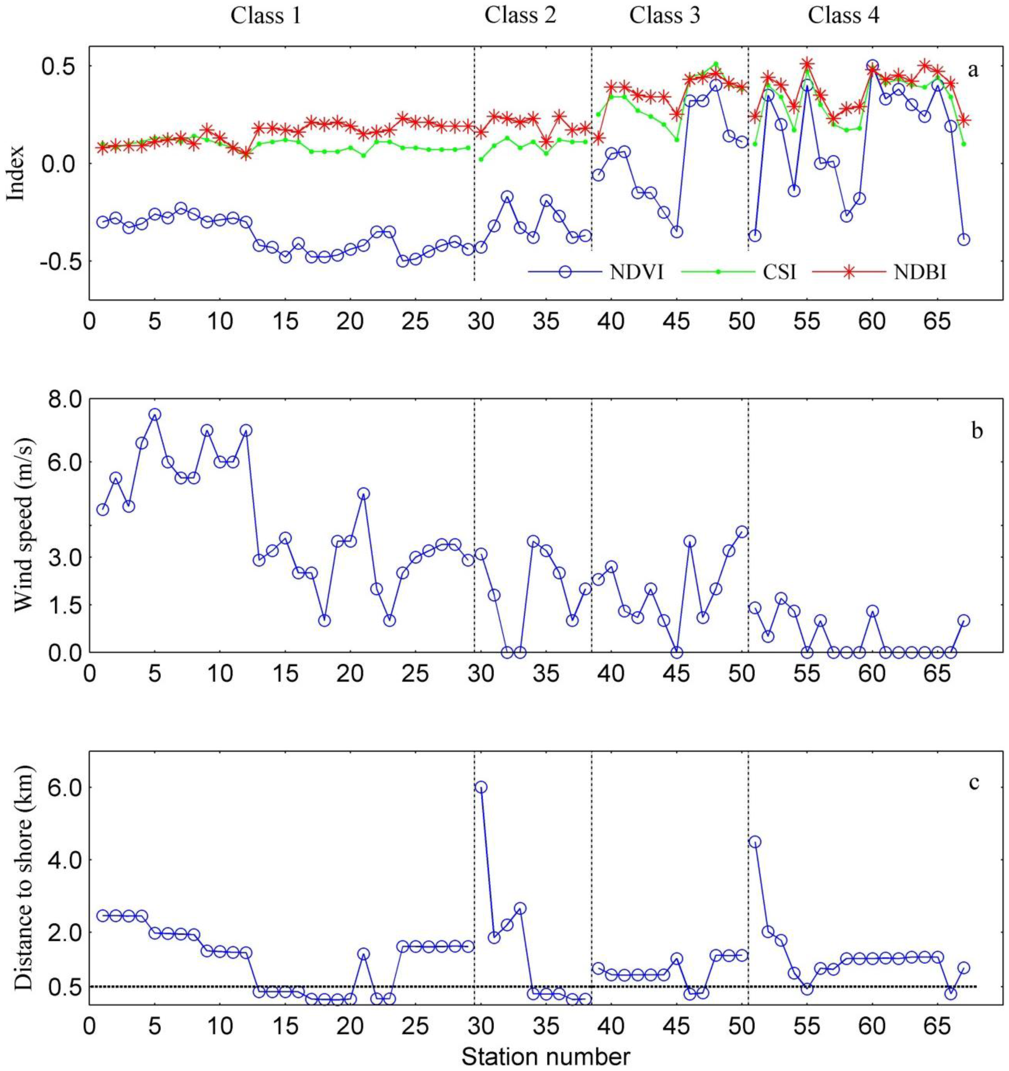
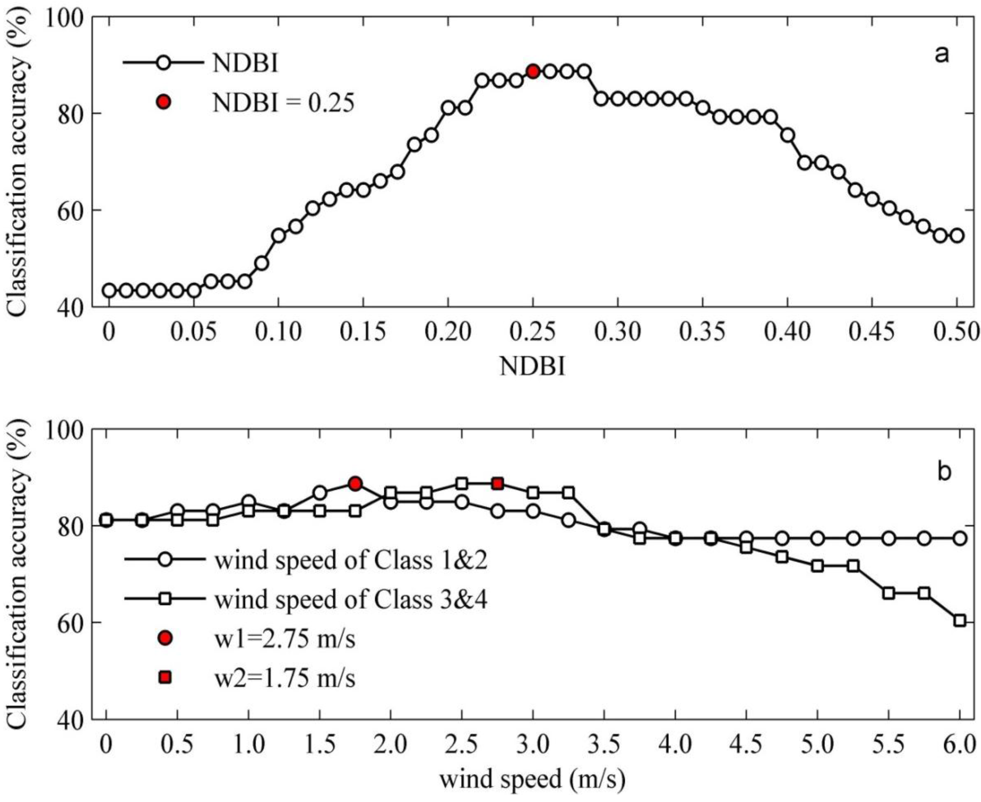
4.2.2. Wind Speed of Different Chla Vertical Profile Classes
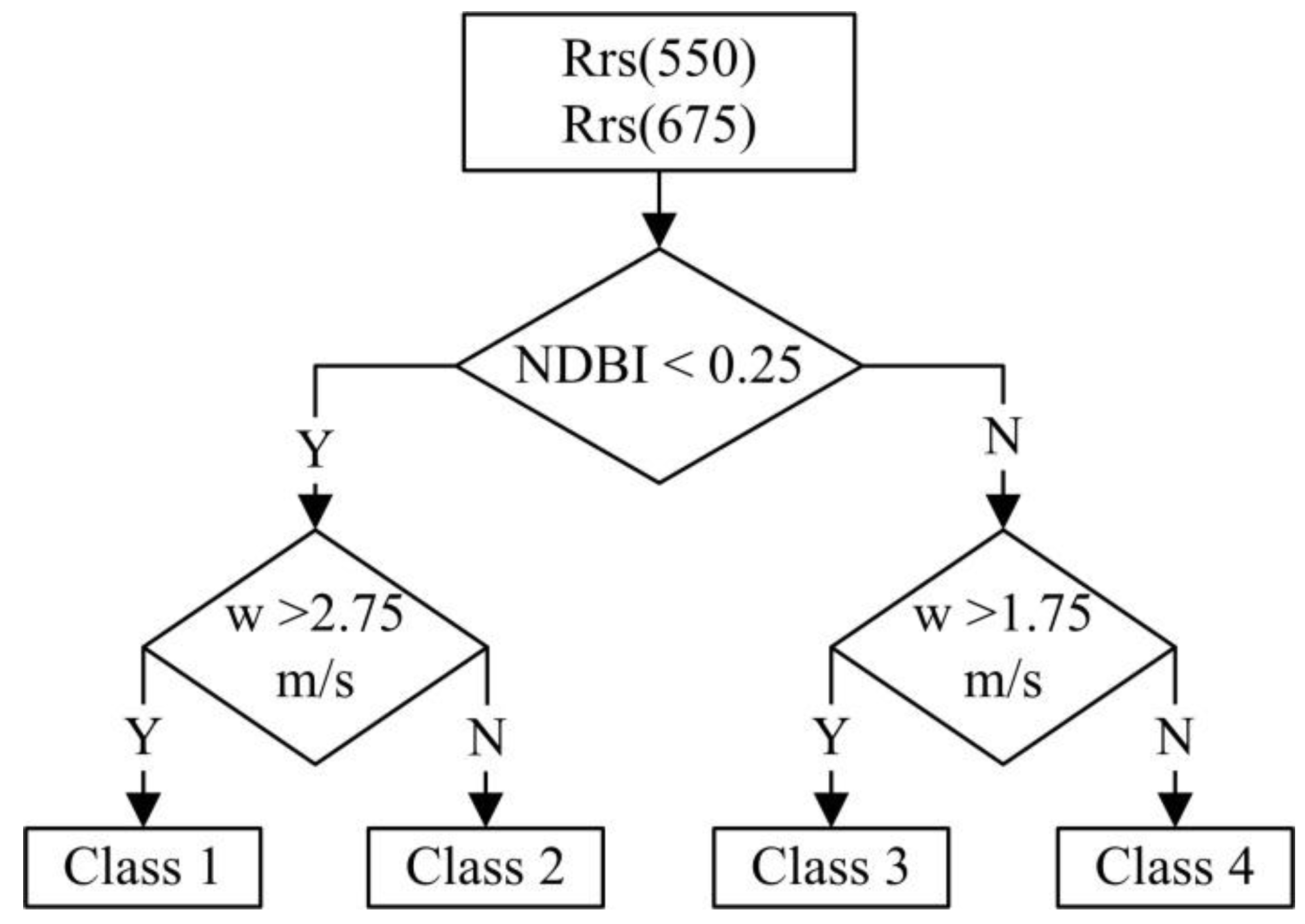
4.2.3. Decision Tree
| Actual | User’s Accuracy | ||||||
|---|---|---|---|---|---|---|---|
| Class 1 | Class 2 | Class 3 | Class 4 | Totals | |||
| Predicted | Class 1 | 19 | 3 | 0 | 0 | 22 | 86% |
| Class 2 | 2 | 4 | 1 | 2 | 9 | 44% | |
| Class 3 | 0 | 0 | 6 | 1 | 7 | 86% | |
| Class 4 | 0 | 1 | 1 | 13 | 15 | 87% | |
| Totals | 21 | 8 | 8 | 16 | 53 | ||
| Producer’s Accuracy | 90% | 50% | 75% | 81% | Overall Acc. | 79% | |
| F1-measure | 88% | 47% | 80% | 84% | Kappa | 0.71 | |
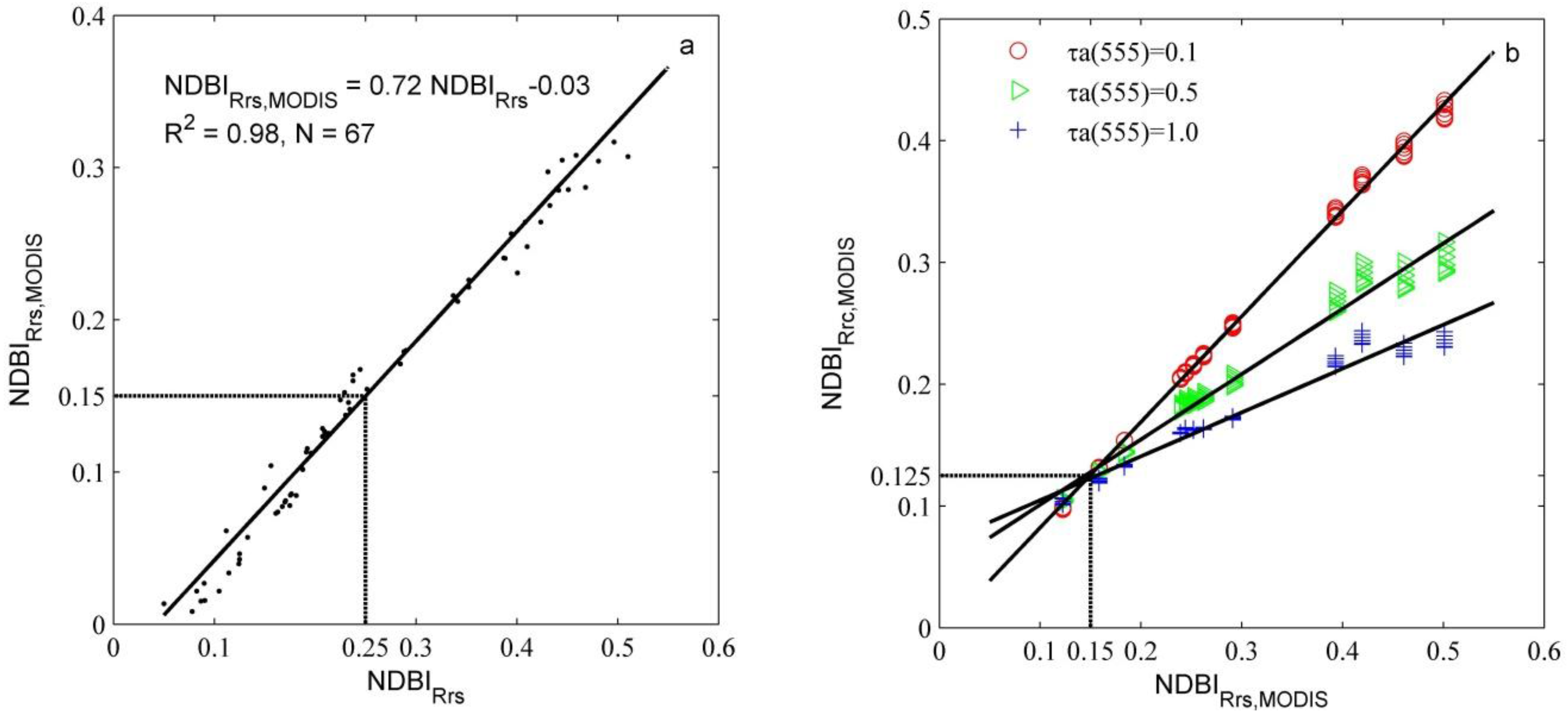
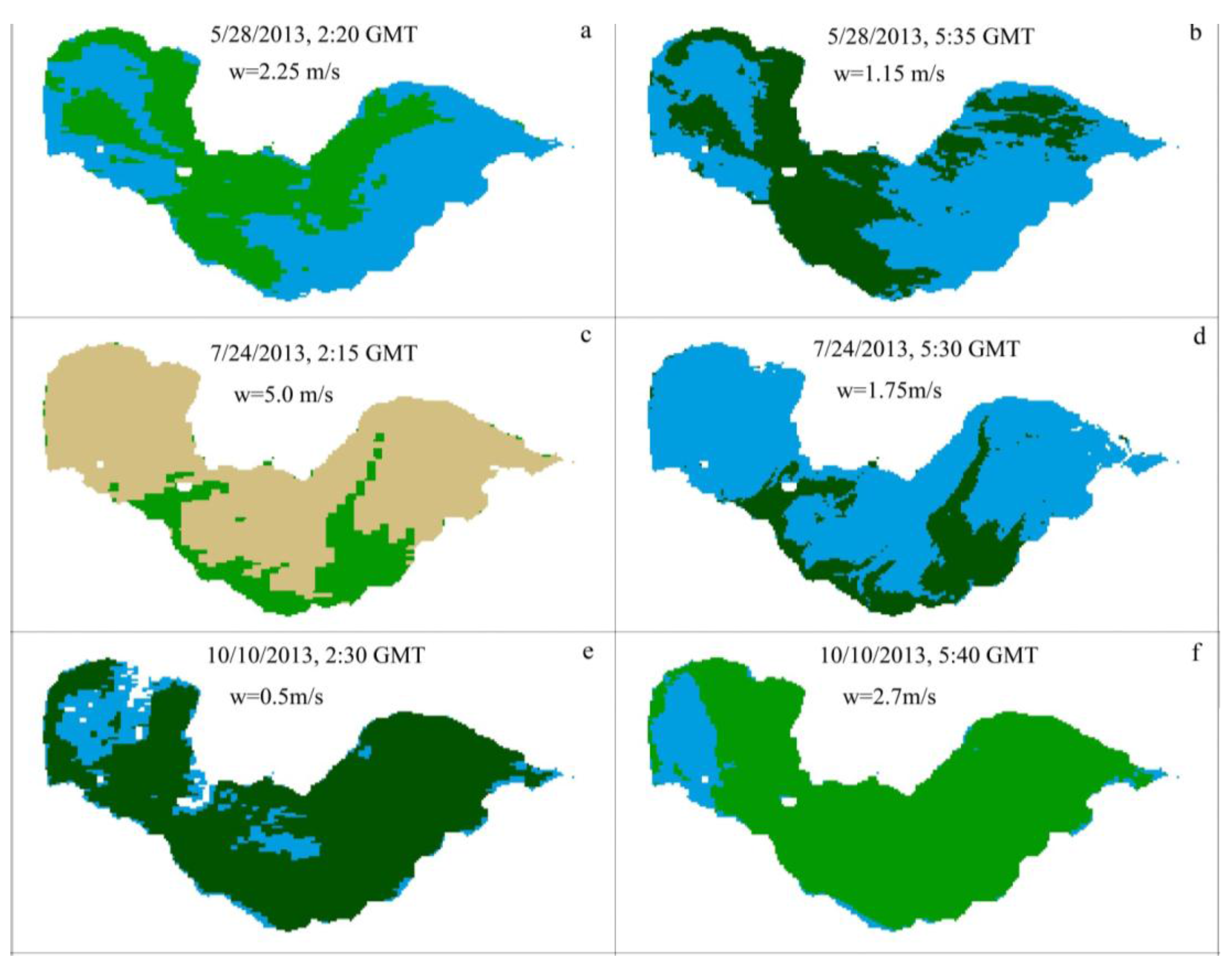
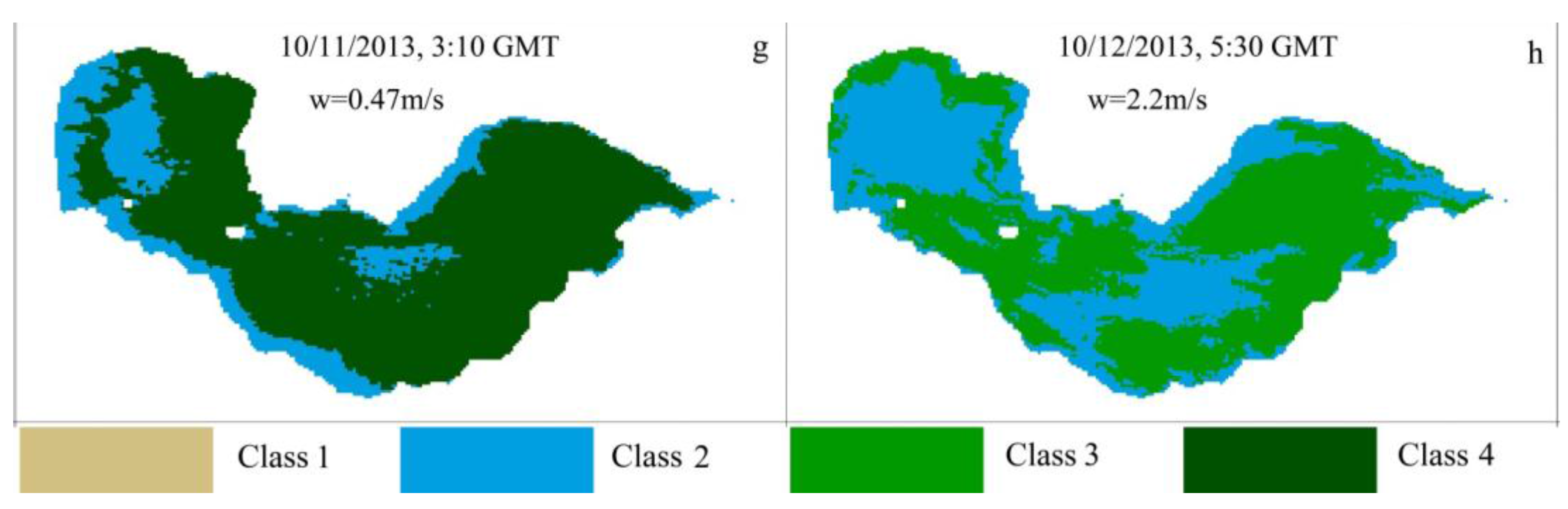
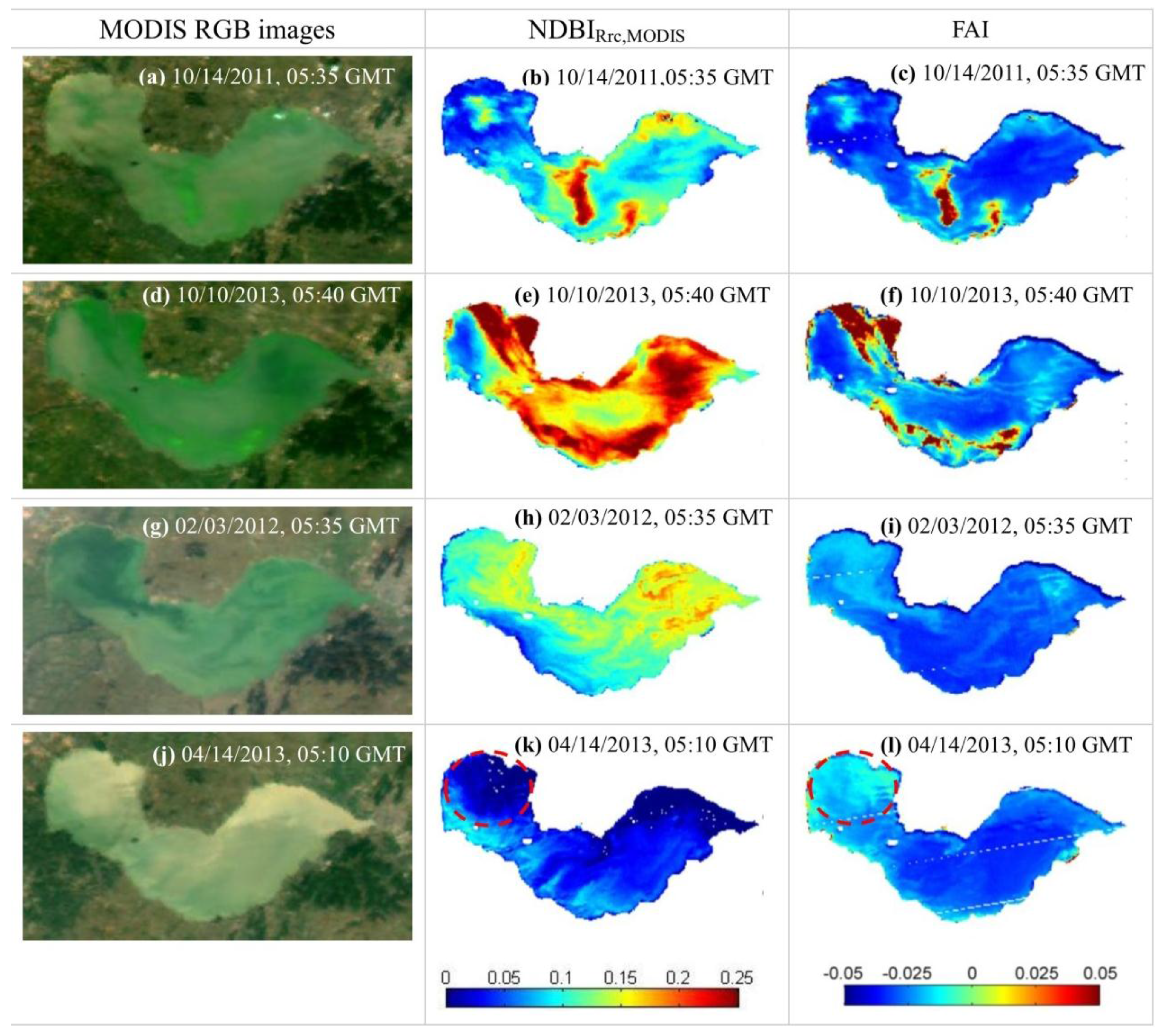
4.3. Identification of Chla Vertical Profile Classes Using MODIS Rrc Data


| Day | GMT Time | Wind Speed (m/s) | NDBIRRC,MODIS | Chla Vertical Class | |
|---|---|---|---|---|---|
| in situ Class | Estimated Class | ||||
| 28 May 2013 | 1:00 | 2.25 | 0.118 | 2 | 2 |
| 28 May 2013 | 2:25 | 2.25 | 0.159 | 4 | 4 |
| 28 May 2013 | 3:25 | 2.25 | 0.160 | 4 | 4 |
| 24 July 2013 | 1:55 | 5.00 | 0.101 | 2 | 1 |
| 24 July 2013 | 2:25 | 5.00 | 0.101 | 2 | 1 |
| 24 July 2013 | 2:55 | 5.00 | 0.101 | 1 | 1 |
| 11 October 2013 | 2:30 | 0.43 | 0.135 | 4 | 4 |
| 11 October 2013 | 3:10 | 0.43 | 0.135 | 4 | 4 |
| 11 October 2013 | 3:50 | 0.43 | 0.135 | 4 | 4 |
| 12 October 2013 | 1:30 | 2.20 | 0.101 | 2 | 2 |
| 12 October 2013 | 2:05 | 2.20 | 0.101 | 2 | 2 |
| 12 October 2013 | 2:40 | 2.20 | 0.101 | 2 | 2 |
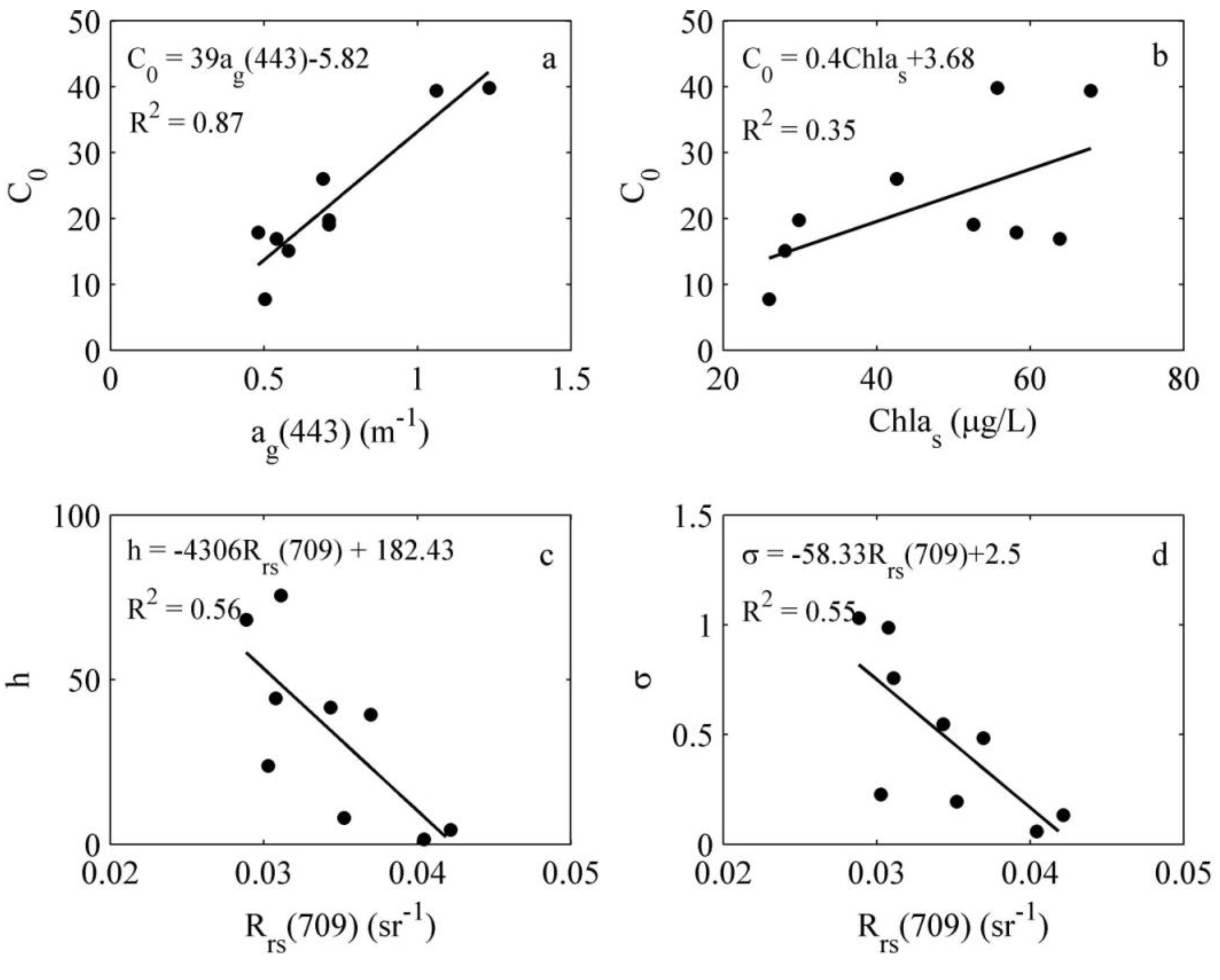
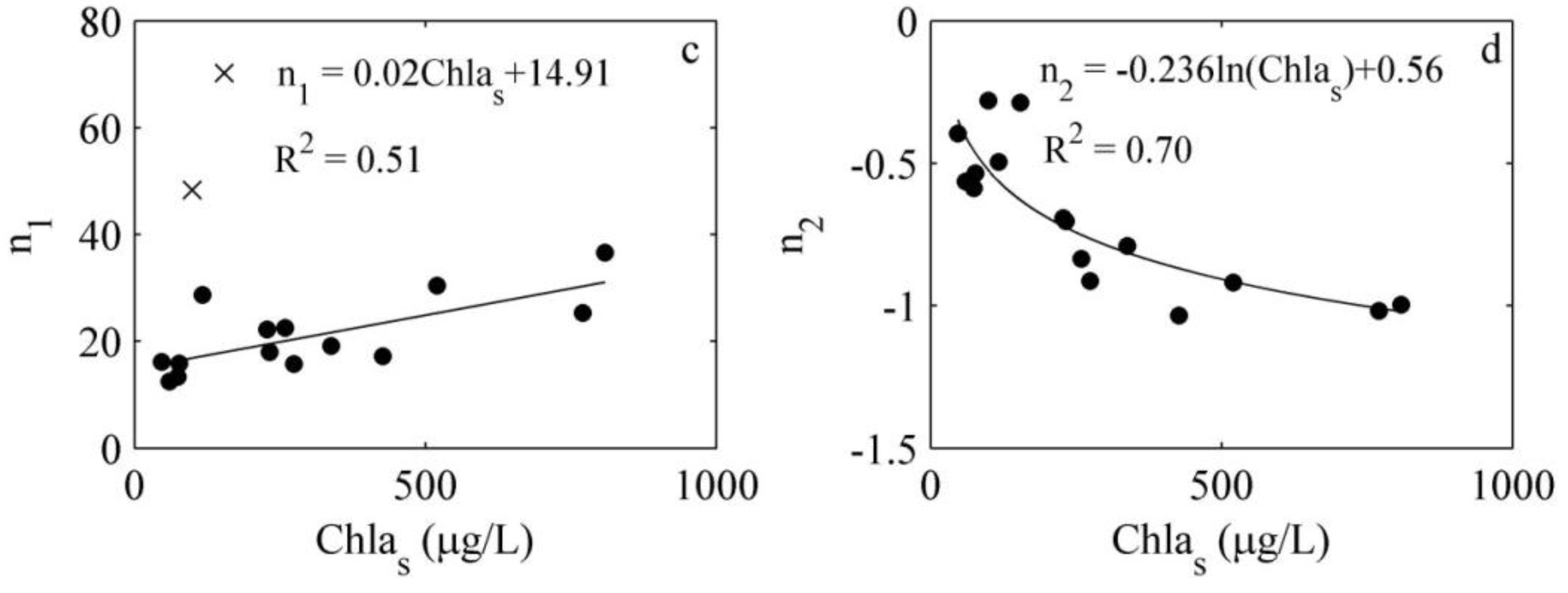
4.4. Relationships of Structure Parameters to Remotely Sensed Data

5. Discussion

6. Conclusion
Acknowledgments
Author Contributions
Conflicts of Interest
References
- Duan, H.; Ma, R.; Xu, X.; Kong, F.; Zhang, S.; Kong, W.; Hao, J.; Shang, L. Two-decade reconstruction of algal blooms in China’s Lake Taihu. Environ. Sci. Technol. 2009, 43, 3522–3528. [Google Scholar] [CrossRef] [PubMed]
- Kahru, M.; Savchuk, O.P.; Elmgren, R. Satellite measurements of cyanobacterial bloom frequency in the Baltic Sea: Interannual and spatial variability. Mar. Ecol. Prog. Ser. 2007, 343, 15–23. [Google Scholar] [CrossRef]
- Siswanto, E.; Ishizaka, J.; Tripathy, S.C.; Miyamura, K. Detection of harmful algal blooms of Karenia mikimotoi using MODIS measurements: A case study of Seto-Inland Sea, Japan. Remote Sens. Environ. 2013, 129, 185–196. [Google Scholar] [CrossRef]
- Tomlinson, M.C.; Stumpf, R.P.; Ransibrahmanakul, V.; Truby, E.W.; Kirkpatrick, G.J.; Pederson, B.A.; Vargo, G.A.; Heil, C.A. Evaluation of the use of SeaWiFS imagery for detecting Karenia brevis harmful algal blooms in the eastern Gulf of Mexico. Remote Sens. Environ. 2004, 91, 293–303. [Google Scholar] [CrossRef]
- Jia, X.; Shi, D.; Shi, M.; Li, R.; Song, L.; Fang, H.; Yu, G. Formation of cyanobacterial blooms in Lake Chaohu and the photosynthesis of dominant species hypothesis. Acta Ecol. Sin. 2011, 31, 2968–2977. [Google Scholar]
- Kutser, T.; Metsamaa, L.; Strömbeck, N.; Vahtmäe, E. Monitoring cyanobacterial blooms by satellite remote sensing. Estuar. Coast. Shelf Sci. 2006, 67, 303–312. [Google Scholar] [CrossRef]
- Odermatt, D.; Pomati, F.; Pitarch, J.; Carpenter, J.; Kawka, M.; Schaepman, M.; Wüest, A. MERIS observations of phytoplankton blooms in a stratified eutrophic lake. Remote Sens. Environ. 2012, 126, 232–239. [Google Scholar] [CrossRef]
- Bresciani, M.; Adamo, M.; De Carolis, G.; Matta, E.; Pasquariello, G.; Vaičiūtė, D.; Giardino, C. Monitoring blooms and surface accumulation of cyanobacteria in the Curonian Lagoon by combining MERIS and ASAR data. Remote Sens. Environ. 2014, 146, 124–135. [Google Scholar] [CrossRef]
- Duan, H.; Ma, R.; Zhang, Y.; Loiselle, S.A.; Xu, J.; Zhao, C.; Zhou, L.; Shang, L. A new three-band algorithm for estimating chlorophyll concentrations in turbid inland lakes. Environ. Res. Lett. 2010, 5. [Google Scholar] [CrossRef]
- Song, K.; Li, L.; Tedesco, L.P.; Li, S.; Duan, H.; Liu, D.; Hall, B.E.; Du, J.; Li, Z.; Shi, K.; et al. Remote estimation of chlorophyll-a in turbid inland waters: Three-band model versus GA-PLS model. Remote Sens. Environ. 2013, 136, 342–357. [Google Scholar] [CrossRef]
- Duan, H.; Ma, R.; Hu, C. Evaluation of remote sensing algorithms for cyanobacterial pigment retrievals during spring bloom formation in several lakes of East China. Remote Sens. Environ. 2012, 126, 126–135. [Google Scholar] [CrossRef]
- Lou, X.; Hu, C. Diurnal changes of a harmful algal bloom in the East China Sea: Observations from GOCI. Remote Sens. Environ. 2014, 140, 562–572. [Google Scholar] [CrossRef]
- Cao, H.; Kong, F.; Luo, L.; Shi, X.; Yang, Z.; Zhang, X.; Tao, Y. Effects of wind and wind-induced waves on vertical phytoplankton distribution and surface blooms of Microcystis aeruginosain Lake Taihu. J. Freshw. Ecol. 2006, 21, 231–238. [Google Scholar] [CrossRef]
- Silulwane, N.F.; Richardson, A.J.; Shillington, F.A.; Mitchell-Innes, B.A. Identification and classification of vertical chlorophyll patterns in the Benguela upwelling system and Angola-Benguela front using an artificial neural network. South Afr. J. Mar. Sci. 2010, 23, 37–51. [Google Scholar] [CrossRef]
- Ndong, M.; Bird, D.; Nguyen-Quang, T.; de Boutray, M.L.; Zamyadi, A.; Vincon-Leite, B.; Lemaire, B.J.; Prevost, M.; Dorner, S. Estimating the risk of cyanobacterial occurrence using an index integrating meteorological factors: Application to drinking water production. Water Res. 2014, 56, 98–108. [Google Scholar] [CrossRef] [PubMed]
- George, D.; Edwards, R. The effect of wind on the distribution of chlorophyll a and crustacean plankton in a shallow eutrophic reservoir. J. Appl. Ecol. 1976, 13, 667–690. [Google Scholar] [CrossRef]
- Webster, I.T.; Hutchinson, P.A. Effect of wind on the distribution of phytoplankton cells in lakes revisited. Limnol. Oceanogr. 1994, 39, 365–373. [Google Scholar] [CrossRef]
- Kanoshina, I.; Lips, U.; Leppänen, J.-M. The influence of weather conditions (temperature and wind) on cyanobacterial bloom development in the Gulf of Finland (Baltic Sea). Harmful Algae 2003, 2, 29–41. [Google Scholar] [CrossRef]
- Huang, C.; Li, Y.; Yang, H.; Sun, D.; Yu, Z.; Zhang, Z.; Chen, X.; Xu, L. Detection of algal bloom and factors influencing its formation in Taihu Lake from 2000 to 2011 by MODIS. Environ. Earth Sci. 2013, 71, 3705–3714. [Google Scholar] [CrossRef]
- Tsujimura, S.; Tsukada, H.; Nakahara, H.; Nakajima, T.; Nishino, M. Seasonal variations of Microcystis populations in sediments of Lake Biwa, Japan. Hydrobiologia 2000, 434, 183–192. [Google Scholar] [CrossRef]
- Walsby, A.; Booker, M. Changes in buoyancy of a planktonic blue-green alga in response to light intensity. Br. Phycol. J. 1980, 15, 311–319. [Google Scholar] [CrossRef]
- Kromkamp, J.; van den Heuvel, A.; Mur, L.R. Formation of gas vesicles in phosphorus-limited cultures of Microcystis aeruginosa. J. Gen. Microbiol. 1989, 135, 1933–1939. [Google Scholar] [CrossRef]
- Klemer, A.; Feuillade, J.; Feuillade, M. Cyanobacterial blooms: carbon and nitrogen limitation have opposite effects on the buoyancy of Oscillatoria. Science 1982, 215, 1629–1631. [Google Scholar] [CrossRef] [PubMed]
- Wynne, T.T.; Stumpf, R.P.; Tomlinson, M.C.; Dyble, J. Characterizing a cyanobacterial bloom in western Lake Erie using satellite imagery and meteorological data. Limnol. Oceanogr. 2010, 55, 2025–2036. [Google Scholar] [CrossRef]
- Morel, A.; Berthon, J.-F. Surface pigments, algal biomass profiles, and potential production of the euphotic layer: Relationships reinvestigated in view of remote-sensing applications. Limnol. Oceanogr. 1989, 34, 1545–1562. [Google Scholar] [CrossRef]
- Xiu, P.; Liu, Y.; Tang, J. Variations of ocean colour parameters with nonuniform vertical profiles of chlorophyll concentration. Int. J. Remote Sens. 2008, 29, 831–849. [Google Scholar] [CrossRef]
- Gordon, H.R.; Clark, D.K. Remote sensing optical properties of a stratified ocean: An improved interpretation. Appl. Opt. 1980, 19, 3428–3430. [Google Scholar] [CrossRef] [PubMed]
- Stramska, M.; Stramski, D. Effects of a nonuniform vertical profile of chlorophyll concentration on remote-sensing reflectance of the ocean. Appl. Opt. 2005, 44, 1735–1747. [Google Scholar] [CrossRef] [PubMed]
- Kutser, T.; Metsamaa, L.; Dekker, A.G. Influence of the vertical distribution of cyanobacteria in the water column on the remote sensing signal. Estuar. Coast. Shelf Sci. 2008, 78, 649–654. [Google Scholar] [CrossRef]
- Sathyendranath, S.; Platt, T.; Caverhill, C.M.; Warnock, R.E.; Lewis, M.R. Remote sensing of oceanic primary production: Computations using a spectral model. Deep Sea Res. Part A. Oceanogr. Res. Pap. 1989, 36, 431–453. [Google Scholar] [CrossRef]
- André, J.-M. Ocean color remote-sensing and the subsurface vertical structure of phytoplankton pigments. Deep Sea Res. Part A. Oceanogr. Res. Pap. 1992, 39, 763–779. [Google Scholar] [CrossRef]
- Millán-Núñez, R.; Alvarez-Borrego, S.; Trees, C.C. Modeling the vertical distribution of chlorophyll in the California Current System. J. Geophys. Res. 1997, 102. [Google Scholar] [CrossRef]
- Hidalgo-Gonzalez, R.M.; Alvarez-Borrego, S. Chlorophyll profiles and the water column structure in the Gulf of California. Oceanol. Acta 2001, 24, 19–28. [Google Scholar] [CrossRef]
- D’Alimonte, D.; Zibordi, G.; Kajiyama, T.; Berthon, J.-F. Comparison between MERIS and regional high-level products in European seas. Remote Sens. Environ. 2014, 140, 378–395. [Google Scholar] [CrossRef]
- Uitz, J.; Claustre, H.; Morel, A.; Hooker, S.B. Vertical distribution of phytoplankton communities in open ocean: An assessment based on surface chlorophyll. J. Geophys. Res. 2006, 111. [Google Scholar] [CrossRef]
- Chen, X.; Yang, X.; Dong, X.; Liu, E. Environmental changes in Chaohu Lake (Southeast, China) since the mid 20th century: The interactive impacts of nutrients, hydrology and climate. Limnol.—Ecol. Manag. Inland Waters 2013, 43, 10–17. [Google Scholar] [CrossRef]
- Lodhi, M.A.; Rundquist, D.C. A spectral analysis of bottom-induced variation in the colour of Sand Hills lakes, Nebraska, USA. Int. J. Remote Sens. 2001, 22, 1665–1682. [Google Scholar] [CrossRef]
- Ma, R.; Tang, J.; Dai, J. Bio-optical model with optimal parameter suitable for Taihu Lake in water colour remote sensing. Int. J. Remote Sens. 2006, 27, 4305–4327. [Google Scholar] [CrossRef]
- Shang, G.P.; Shang, J.C. Spatial and temporal variations of eutrophication in Western Chaohu Lake, China. Environ. Monit. Assess. 2007, 130, 99–109. [Google Scholar] [CrossRef] [PubMed]
- Chen, X.; Yang, X.; Dong, X.; Liu, Q. Nutrient dynamics linked to hydrological condition and anthropogenic nutrient loading in Chaohu Lake (Southeast China). Hydrobiologia 2010, 661, 223–234. [Google Scholar] [CrossRef]
- Liu, W.; Qiu, R. Water eutrophication in China and the combating strategies. J. Chem. Technol. Bio. Technol. 2007, 82, 781–786. [Google Scholar] [CrossRef]
- Yu, T. Phytoplankton Community Structure in Chaohu Lake. Master’s Thesis, Anhui University, Hefei, China, 10 June 2010. [Google Scholar]
- Chen, Z.; Li, Y.; Pan, J. Distributions of colored dissolved organic matter and dissolved organic carbon in the Pearl River Estuary, China. Cont. Shelf Res. 2004, 24, 1845–1856. [Google Scholar] [CrossRef]
- Jiang, G.; Ma, R.; Loiselle, S.A.; Duan, H. Optical approaches to examining the dynamics of dissolved organic carbon in optically complex inland waters. Environ. Res. Lett. 2012, 7. [Google Scholar] [CrossRef]
- Mueller, J.L.; McClain, G.S.F.C.R.; Mueller, J.; Bidigare, R.; Trees, C.; Balch, W.; Dore, J.; Drapeau, D.; Karl, D.; Van, L.H. Ocean optics protocols for satellite ocean color sensor validation, revision 5, volume V: Biogeochemical and bio-optical measurements and data analysis protocols. NASA Tech. Memo. 2003, 211621, 1–36. [Google Scholar]
- Mobley, C.D. Estimation of the remote-sensing reflectance from above-surface measurements. Appl. Opt. 1999, 38, 7442–7455. [Google Scholar] [CrossRef] [PubMed]
- Qi, L.; Hu, C.; Duan, H.; Barnes, B.; Ma, R. An EOF-Based algorithm to estimate chlorophyll a concentrations in Taihu Lake from MODIS land-band measurements: Implications for near real-time applications and forecasting models. Remote Sens. 2014, 6, 10694–10715. [Google Scholar] [CrossRef]
- Qi, L.; Hu, C.; Duan, H.; Cannizzaro, J.; Ma, R. A novel MERIS algorithm to derive cyanobacterial phycocyanin pigment concentrations in a eutrophic lake: Theoretical basis and practical considerations. Remote Sens. Environ. 2014, 154, 298–317. [Google Scholar] [CrossRef]
- Feng, L.; Hu, C.; Chen, X.; Tian, L.; Chen, L. Human induced turbidity changes in Poyang Lake between 2000 and 2010: Observations from MODIS. J. Geophys. Res. 2012. [Google Scholar] [CrossRef]
- Rouse, J.W.; Haas, R.H.; Schell, J.A.; Deering, D.W. Monitoring vegetation systems in the Great Plains with ERTS. NASA Spec. Publ. 1974, 351, 309. [Google Scholar]
- Li, J.; Wu, D.; Wu, Y.; Liu, H.; Shen, Q.; Zhang, H. Identification of algae-bloom and aquatic macrophytes in Lake Taihu from in situ measured spectra data. J. Lake Sci. 2009, 21, 215–222. [Google Scholar] [CrossRef]
- Hu, C. A novel ocean color index to detect floating algae in the global oceans. Remote Sens. Environ. 2009, 113, 2118–2129. [Google Scholar] [CrossRef]
- Breiman, L.; Friedman, J.; Stone, C.J.; Olshen, R.A. Classification and Regression Trees; CRC Press: Florida, FL, USA, 1984. [Google Scholar]
- Razi, M.A.; Athappilly, K. A comparative predictive analysis of neural networks (NNs), nonlinear regression and classification and regression tree (CART) models. Expert Syst. Appl. 2005, 29, 65–74. [Google Scholar] [CrossRef]
- Cózar, A.; Gálvez, J.A.; Hull, V.; García, C.M.; Loiselle, S.A. Sediment resuspension by wind in a shallow lake of Esteros del Iberá (Argentina): A model based on turbidimetry. Ecol. Model. 2005, 186, 63–76. [Google Scholar] [CrossRef]
- Bengio, Y.; Grandvalet, Y. No unbiased estimator of the variance of k-fold cross-validation. J. Mach. Learn. Res. 2003, 5, 1089–1105. [Google Scholar]
- Shi, K.; Li, Y.; Li, L.; Lu, H. Absorption characteristics of optically complex inland waters: Implications for water optical classification. J. Geophys. Res.: Biogeosci. 2013, 118, 860–874. [Google Scholar] [CrossRef]
- Gower, J.F.R.; Doerffer, R.; Borstad, G.A. Interpretation of the 685 nm peak in water-leaving radiance spectra in terms of fluorescence, absorption and scattering, and its observation by MERIS. Int. J. Remote Sens. 1999, 20, 1771–1786. [Google Scholar] [CrossRef]
- Gower, J.; King, S.; Wei, Y.; Borstad, G.; Brown, L. Use of the 709 nm band of MERIS to detect intense plankton blooms and other conditions in coastal waters. In Proceedings of the MERIS User Workshop, Frascati, Italy, 10–13 November 2003.
- Gitelson, A.A.; Dall’Olmo, G.; Moses, W.; Rundquist, D.C.; Barrow, T.; Fisher, T.R.; Gurlin, D.; Holz, J. A simple semi-analytical model for remote estimation of chlorophyll-a in turbid waters: Validation. Remote Sens. Environ. 2008, 112, 3582–3593. [Google Scholar] [CrossRef]
- Bailey, S.W.; Werdell, P.J. A multi-sensor approach for the on-orbit validation of ocean color satellite data products. Remote Sens. Environ. 2006, 102, 12–23. [Google Scholar] [CrossRef]
- Ma, R.; Jiang, G.; Duan, H.; Bracchini, L.; Loiselle, S. Effective upwelling irradiance depths in turbid waters: A spectral analysis of origins and fate. Opt. Express 2011, 19, 7127–7138. [Google Scholar] [CrossRef] [PubMed]
- Gordon, H.R. Atmospheric correction of ocean color imagery in the Earth Observing System era. J. Geophys. Res.: Atmos. (1984–2012) 1997, 102, 17081–17106. [Google Scholar] [CrossRef]
- Wang, M.; Shi, W. Estimation of ocean contribution at the MODIS near—Infrared wavelengths along the east coast of the US: Two case studies. Geophys. Res. Lett. 2005. [Google Scholar] [CrossRef]
- Carvalho, D.; Rocha, A.; Gómez-Gesteira, M.; Alvarez, I.; Silva Santos, C. Comparison between CCMP, QuikSCAT and buoy winds along the Iberian Peninsula coast. Remote Sens. Environ. 2013, 137, 173–183. [Google Scholar] [CrossRef]
- Lin, H.; Xu, Q.; Zheng, Q. An overview on SAR measurements of sea surface wind. Prog. Nat. Sci. 2008, 18, 913–919. [Google Scholar] [CrossRef]
- Hunter, P.; Tyler, A.; Willby, N.; Gilvear, D. The spatial dynamics of vertical migration by Microcystis aeruginosa in a eutrophic shallow lake: A case study using high spatial resolution time—Series airborne remote sensing. Limnol. Oceanogr. 2008, 53, 2391–2406. [Google Scholar] [CrossRef]
- Loiselle, S.; Cozar, A.; Adgo, E.; Ballatore, T.; Chavula, G.; Descy, J.P.; Harper, D.M.; Kansiime, F.; Kimirei, I.; Langenberg, V. Decadal trends and common dynamics of the bio-optical and thermal characteristics of the African Great Lakes. PloS One 2014, 9. [Google Scholar] [CrossRef] [PubMed]
© 2015 by the authors; licensee MDPI, Basel, Switzerland. This article is an open access article distributed under the terms and conditions of the Creative Commons Attribution license (http://creativecommons.org/licenses/by/4.0/).
Share and Cite
Xue, K.; Zhang, Y.; Duan, H.; Ma, R.; Loiselle, S.; Zhang, M. A Remote Sensing Approach to Estimate Vertical Profile Classes of Phytoplankton in a Eutrophic Lake. Remote Sens. 2015, 7, 14403-14427. https://doi.org/10.3390/rs71114403
Xue K, Zhang Y, Duan H, Ma R, Loiselle S, Zhang M. A Remote Sensing Approach to Estimate Vertical Profile Classes of Phytoplankton in a Eutrophic Lake. Remote Sensing. 2015; 7(11):14403-14427. https://doi.org/10.3390/rs71114403
Chicago/Turabian StyleXue, Kun, Yuchao Zhang, Hongtao Duan, Ronghua Ma, Steven Loiselle, and Minwei Zhang. 2015. "A Remote Sensing Approach to Estimate Vertical Profile Classes of Phytoplankton in a Eutrophic Lake" Remote Sensing 7, no. 11: 14403-14427. https://doi.org/10.3390/rs71114403
APA StyleXue, K., Zhang, Y., Duan, H., Ma, R., Loiselle, S., & Zhang, M. (2015). A Remote Sensing Approach to Estimate Vertical Profile Classes of Phytoplankton in a Eutrophic Lake. Remote Sensing, 7(11), 14403-14427. https://doi.org/10.3390/rs71114403