Classification of Several Optically Complex Waters in China Using in Situ Remote Sensing Reflectance

Abstract

Determining the dominant optically active substances in water bodies via classification can improve the accuracy of bio-optical and water quality parameters estimated by remote sensing. This study provides four robust centroid sets from in situ remote sensing reflectance (R_rs (λ)) data presenting typical optical types obtained by plugging different similarity measures into fuzzy c-means (FCM) clustering. Four typical types of waters were studied: (1) highly mixed eutrophic waters, with the proportion of absorption of colored dissolved organic matter (CDOM), phytoplankton, and non-living particulate matter at approximately 20%, 20%, and 60% respectively; (2) CDOM-dominated relatively clear waters, with approximately 45% by proportion of CDOM absorption; (3) nonliving solids-dominated waters, with approximately 88% by proportion of absorption of nonliving particulate matter; and (4) cyanobacteria-composed scum. We also simulated spectra from seven ocean color satellite sensors to assess their classification ability. POLarization and Directionality of the Earth's Reflectances (POLDER), Sentinel-2A, and MEdium Resolution Imaging Spectrometer (MERIS) were found to perform better than the rest. Further, a classification tree for MERIS, in which the characteristics of R_rs (709)/R_rs (681), R_rs (560)/R_rs (709), R_rs (560)/R_rs (620), and R_rs (709)/R_rs (761) are integrated, is also proposed in this paper. The overall accuracy and Kappa coefficient of the proposed classification tree are 76.2% and 0.632, respectively.

1. Introduction

Remote sensing reflectance from the surface of optically complex waters is comprised of the backscattering from optically active constituents, including pure water, phytoplankton, nonliving solids, and colored dissolved organic matter (CDOM). In addition to containing more than one type of constituent, optically complex waters are characterized by a high degree of spatiotemporal diversity in their optical properties. Using remote sensing to classify such waters according to their optical properties will help identify optically complex waters and understand biogeochemical processes therein. A number of recent works have developed optical pre-classification schemes aiming to select regional inversion algorithms for water constituents [1,2,3]. Several studies in the literature have focused on the development of such local or regional inversion algorithms for China’s waters [4,5,6,7,8,9,10,11]. These are limited, however, by their high dependency on the dataset used for algorithm development, and local or regional findings therefore tend not to be applicable elsewhere or to larger scales.

Early studies aiming to identify water types made use of their color. In the beginning, oceans were classified into two types: Case I was blue clear ocean waters and Case II was in different colors caused by increasing turbidity [12,13,14]. Case I comprised open ocean waters with all constituents co-varying with phytoplankton. Case II had been expanded to comprise all other natural waters. It was subsequently proposed that waters could be classified as optically shallow or optically deep, depending on whether or not bottom reflectance contributed to the water-leaving reflectance [15,16]. Most water constituent algorithms are intended for optically deep waters. In recent years, optically complex waters have been classified by remote sensing into several distinct types, such as phytoplankton-dominated, suspended solids-dominated, and other mixed waters [2,3].

Previous studies classified waters based on different types of parameters. Many [17,18] developed optical classification schemes based mainly on light penetration parameters, including euphotic zone depths (EZD), Secchi depth (SD), the spectral irradiance reflectance (R), the total attenuation coefficient (c), the diffuse attenuation coefficient for downwelling irradiance (Kd), and their ratio (Kd/c). Some studies classified waters using only water quality parameters (e.g., SD, turbidity, chlorophyll-a concentration (chl-a), yellow substance, and sea surface temperature) [19] or inherent optical properties (IOPs; e.g., absorption and scattering coefficients) [15,20,21,22]. Some studies used a combination of water quality parameters and optical properties [21,23,24]. Classification results tend to improve as more parameters of different types (i.e., water quality parameters, IOPs, and apparent optical parameters (AOPs)) are included as inputs. However, the extensive parameterization possible to achieve through in situ measurements is inefficient. An operational approach to surface water classification makes use of remote sensing reflectance (R_rs (λ)) or irradiance reflectance (R (λ)) [2,25,26,27,28,29], which can be obtained directly from satellite images.

Feature-based methods are often adopted when using R_rs (λ) to classify waters. The related research has used supervised classifiers, such as decision trees, maximum likelihood, supervised neural networks, or support vector machines [19,30] and unsupervised classification, based on K-means or fuzzy c-means (FCM) clustering [27,31,32,33,34], hierarchical algorithms [11,25], unsupervised neural networks [35], or eigenvector classifiers using variance analysis [2,36]. Unsupervised classification is based on the data alone and characterized by less human interference than supervised classification. Furthermore, many researchers have attempted to classify water types using R_rs (λ) alone [1,2,26,32,37], which has been associated with some algorithm improvement. Vantrepotte et al. [2] applied an unsupervised classification method developed by Ward [38] to divide data into homogeneous groups. Vantrepotte and Mélin [3] used the iterative self-organizing data analysis technique (ISODATA) clustering method. The above clustering methods could not provide class memberships simultaneously. Moore et al. [1,27] first determined the optimal number of classes using a suite of cluster validity functions, and then applied the FCM algorithm to return the centroid sets for a number of classes and a membership function matrix, which expressed the likelihood that a point, with its observed reflectance vector, belongs to a class with a known R_rs (λ) vector. The method in the current work is primarily based on Moore’s clustering framework, but with minor improvements.

Similar applications of optical classification dedicated to the global scale or coastal ocean are currently limited [1,2,3,33]. Vantrepotte and Mélin [3] optically classified global coastal ocean, from very turbid to oligotrophic conditions, and analyzed optical diversity using a global seven-year SeaWiFS data set. In this study, the samples were collected from Chinese eutrophic lakes, reservoirs, and coastal waters, and exhibit large variations in water quality parameters. Our samples span four orders of magnitude of chl-a (0.0139–943 mg·m⁻³), two of TSS (3.00–300 g·m⁻³), and one of CDOM absorption at 440 nm (0.138–4.79 m⁻¹). Many studies observed in situ reflectance spectra and defined typical classes of waters based on researcher experience [8,37]. In contrast, subjectivity can be reduced by clustering in situ reflectance and using the centroid reflectance of the resulting water types in classification. However, methods based on mathematical algorithms typically lack an underlying physical mechanism. Few studies have focused specifically on first clustering R_rs (λ) and then using IOPs and water quality parameters to support the classification results [2,32,33].

The primary objective of this study is to classify several optically complex waters found in China using R_rs (λ). Further, the classification method presented here could inform future classification efforts in similar settings. Fuzzy clustering is used to provide a set of centroids from in situ R_rs (λ) representing typical optical types. IOPs and water quality parameters are then used to validate which water type each cluster represents. The conceptual model of the study is comprised of four parts (Figure 1). In the first, fuzzy clustering is applied to all in situ R_rs (λ) spectra at least twice. Each time, a different similarity measurement was used and new centroid sets were extracted. The centroid sets corresponding to Class i (i = 1, 2, …, c) were intersected to form the final robust centroid sets. In the second part of the study, relationships between R_rs (λ) characteristics of the centroids and environmental parameters of each class were assessed, which indicates the reasonability of the proposed centroids. The given centroid sets represent different types of optically complex waters. Based on the clustering results, a classification tree was proposed in the third part of the study. Finally, the ability of seven ocean color radiometers to discriminate the given optical water types was assessed.

Figure 1. Conceptual model of the study is comprised of four parts. (1) Fuzzy clustering was applied to all in situ R_rs (λ) spectra to form the final robust centroid sets. (2) The relationships between the R_rs (λ) characteristics and environmental parameters of each class were assessed. (3) A classification tree was proposed for hyperspectral sensors. (4) The ability of seven ocean color radiometers to differentiate the given optical water types was assessed.

Figure 1. Conceptual model of the study is comprised of four parts. (1) Fuzzy clustering was applied to all in situ R_rs (λ) spectra to form the final robust centroid sets. (2) The relationships between the R_rs (λ) characteristics and environmental parameters of each class were assessed. (3) A classification tree was proposed for hyperspectral sensors. (4) The ability of seven ocean color radiometers to differentiate the given optical water types was assessed.

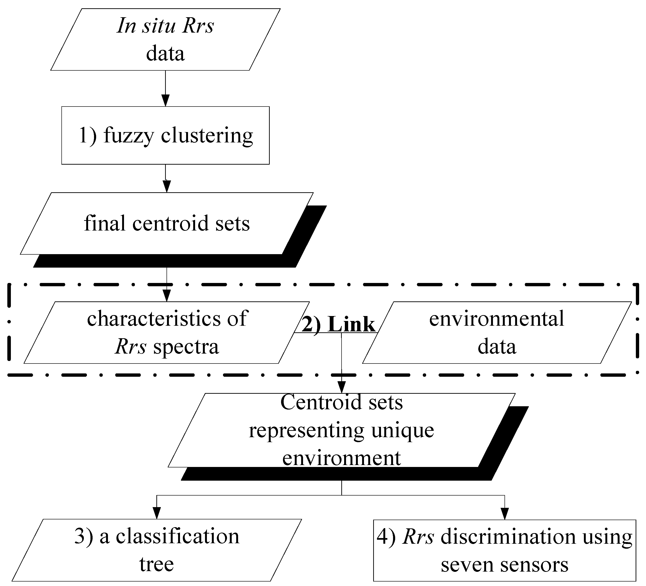
2. Materials and Methods

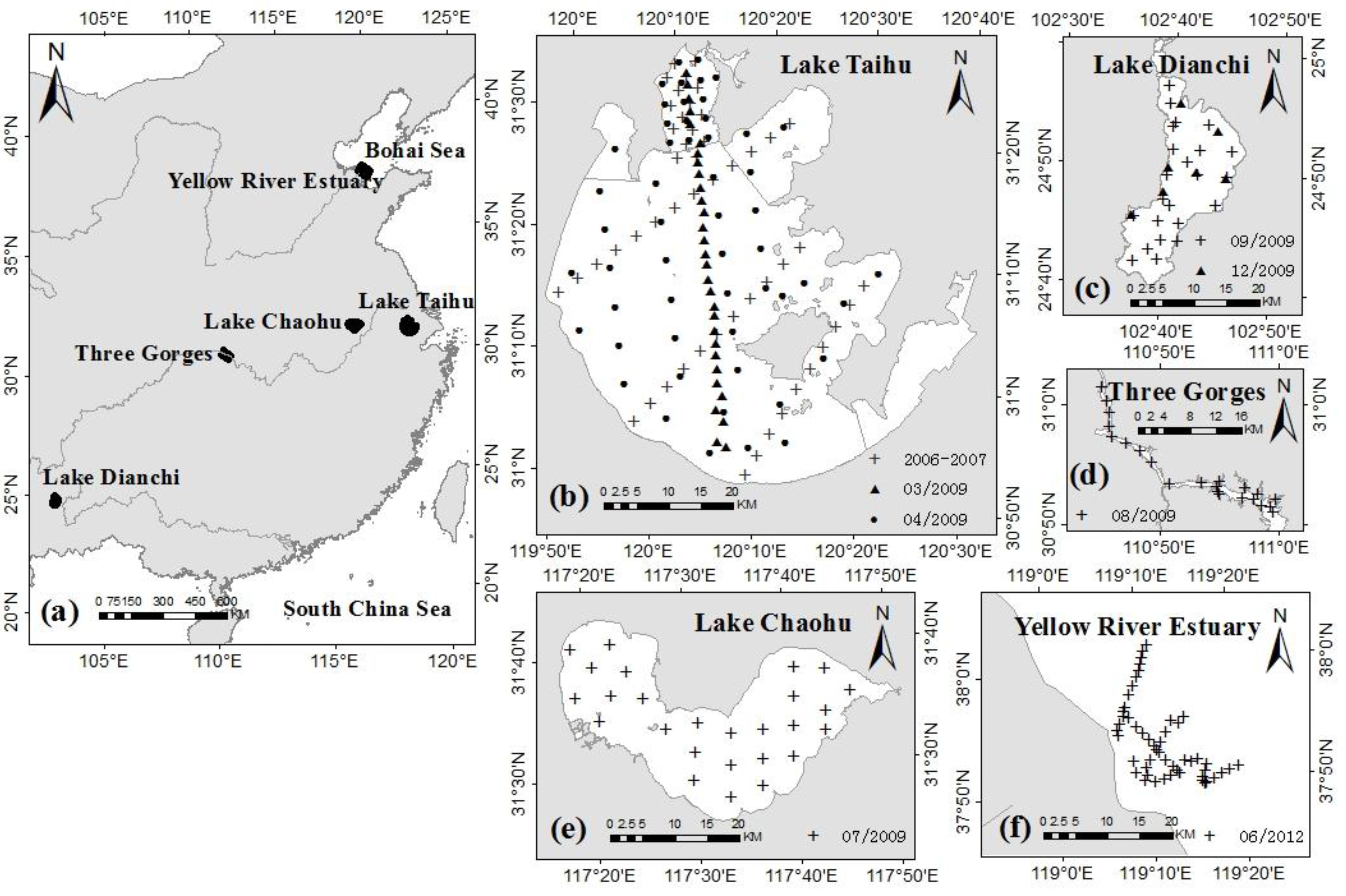
2.1. Data Acquisition and Processing

Collected data consist of R_rs (λ), the concentrations of optically active substances, and the IOPs of the water at each station. Data were obtained from 447 stations during 12 cruises between 2006 and 2012. These stations are located in several typical Chinese optically complex waters, including the Three Gorges Reservoir, Lake Chaohu, Lake Dianchi, Lake Taihu, and the Yellow River estuary (Figure 2). Data from Lake Taihu were obtained by Zhang et al. [4,39,40] in January, July, and October 2006, and January, and April 2007. Data from Lake Chaohu (June 2009), Lake Taihu (March and April 2009), the Three Gorges Reservoir (August, 2009), and Lake Dianchi (September and December 2009) were obtained by Sun et al. [41], and data from the Yellow River estuary were obtained by Zhang et al. [42] in June 2012. An independent test data set, comprising 143 in situ R_rs (λ), was collected from the above areas during other cruises.

Figure 2. (a) Locations of the five study areas. (b) Locations of the field measurement stations in Lake Taihu. Crosses represent the same stations sampled in January, April, and October 2006, and January and April 2007. Triangles represent the stations sampled in March 2009. Circles represent the stations sampled in April 2009. (c) As in (b) Field measurement station locations in Lake Dianchi. Crosses and triangles are the stations sampled in September 2009 and December 2009 respectively. (d) Field measurement stations in the Three Gorges Reservoir. (e) Field measurement stations in Lake Chaohu. (f) Field measurement stations in the Yellow River estuary.

Figure 2. (a) Locations of the five study areas. (b) Locations of the field measurement stations in Lake Taihu. Crosses represent the same stations sampled in January, April, and October 2006, and January and April 2007. Triangles represent the stations sampled in March 2009. Circles represent the stations sampled in April 2009. (c) As in (b) Field measurement station locations in Lake Dianchi. Crosses and triangles are the stations sampled in September 2009 and December 2009 respectively. (d) Field measurement stations in the Three Gorges Reservoir. (e) Field measurement stations in Lake Chaohu. (f) Field measurement stations in the Yellow River estuary.

R_rs (λ) was measured following the above-water method described by Mueller et al. [43], using an ASD FieldSpecR 3 spectroradiometer, with a spectral range of 350–2500 nm, a spectral resolution of 3 nm at 700 nm, and a sampling interval of 1.4 nm over the spectral range 350–1000 nm. Radiance spectra were collected ten times each for a reference panel, the water, and the sky at each station, and were then visually examined to eliminate abnormal spectra. The retained spectra from each station were averaged and R_rs (λ) derived according to Equation (1):

R_rs (λ) = (L_t (λ) – r × L_sky (λ))/(L_p (λ) × π/ρ_p)

(1)

where L_t (λ) is the total upwelling spectral radiance above the water surface; r × L_sky (λ) is the direct upwelling radiance reflected on the water surface contributed by the sky; r is calculated from the Fresnel formula; L_p (λ) is the simultaneously observed radiance of the reference panel, which has an accurately calibrated reflectance, ρ_p, of approximately 30%. The R_rs (λ) measurement error is less than 5%.

Optically active substances considered in this study include chl-a (mg·m⁻³), TSS (g·m⁻³), particulate inorganic matter (PIM, g·m⁻³), particulate organic matter (POM, g·m⁻³), and dissolved organic carbon (DOC, g·m⁻³). Water samples for chl-a measurement were filtered using Whatman GF/C fiberglass filters with a 0.7 µm pore size. chl-a was extracted using 80 °C ethanol (90%), and analyzed spectrophotometrically at 750 and 665 nm, with correction for phaeopigments [44,45]. For the TSS measurements, water samples were filtered through Whatman GF/C fiberglass filters with a 0.7 µm pore size, precombusted at 550 °C for 4 h and weighed using an electrobalance with an accuracy of 10⁻⁴ g. The filtered samples were dried at 105 °C for 4 h, weighed, and filter weights were subtracted to obtain only the sample weights. Next, filtered samples were recombusted at 550 °C for 4 h and reweighed to obtain the PIM value; POM was obtained by subtracting PIM from TSS. The DOC was obtained using a 1020 Total Organic Carbon Analyzer after filtering with Whatman GF/F fiberglass filters.

The IOPs considered include the beam attenuation coefficient of particles and CDOM (c_pg (λ), m⁻¹), the absorption of CDOM (a_CDOM (λ), m⁻¹), the absorption of particles (a_p (λ), m⁻¹), the absorption of non-pigmented particulate matter (a_d (λ), m⁻¹), the absorption of phytoplankton (a_ph (λ), m⁻¹), and the scattering coefficient of particles (b_p (λ), m⁻¹). The above parameters were measured following the NASA ocean optics protocols [39]. The c_pg (λ) and a_CDOM (λ) values were obtained from soluble absorption samples using a Shimadzu UV2401PC UV-Vis spectrophotometer. For a_CDOM (λ), the water samples were first filtered through Millipore isopore membrane filters with a 0.2 µm pore size to remove particulate material. The a_p (λ), a_d (λ), and a_ph (λ) values were obtained using the quantitative filter technique (QFT) [46]. The value of b_p (λ) was obtained by subtracting a_p (λ) and a_CDOM (λ) from c_pg (λ).

2.2. Classification of R_rs (λ) Spectra

In situ R_rs (λ) spectra with similar features were classed together through the FCM algorithm [34,47], which returns a membership function matrix. The centroid sets for a number of classes were obtained via the class memberships. The following three-step clustering framework was adopted. The second step with Principal Component Analysis (PCA) transform and the third step based on more than one similarity measure constituted improvements on the classification method proposed by Moore et al. [1,24].

In the first step, the number of clusters, c, needs to be provided as an input to the FCM clustering routine. The optimal value for c was assessed by two cluster validity measures, the Bayesian information criterion (BIC) index [48] and Dunn’s index [49]. In addition, the value of fuzziness m was two [50].

In the second step, PCA was used to reduce the dimensionality of the in situ R_rs (λ). Using too many bands of in situ R_rs (λ) may lead to a decline in classification accuracy; therefore, we applied PCA transform to acquire an optimal feature subset.

In the last step, the FCM routine was applied to the principal components from the R_rs (λ) of the 447 samples. Each time, clustering was performed based on different similarity measures, such as Euclidean distance (ED), spectral angle distances (SAD), orthogonal projection divergence (OPD) [51], and transformed divergence (TD) [52]. For each FCM routine, c membership grades were obtained for each point in the c clustering groups. When a grade corresponding to Class i is larger, the likelihood that the pixel belongs to Class i is greater (where i =1, 2, …, c). Samples with any one membership grade greater than 0.9 would be attributed to the corresponding centroid set. After running the four routines (ED, SAD, OPD, TD), four centroid sets driven from four similarity measures corresponding to Class i were formed. In each centroid set every point was viewed as a vector. The same vectors appearing in all four centroid sets were selected to form the Class i centroid set (where i = 1, 2, …, c). Finally, c centroid sets were formed, which were much more robust than the centroid sets based on only one similarity measure.

Here the four similarity measures, SAD, ED, OPD, and TD, were defined as:

$$\text{SAD=1-arccos}\frac{x_r^T{x}_c}{\sqrt{(x_r^T{x}_r)(x_c^T{x}_c)}}$$

(2)

$$\text{ED=}\Vert x_r-x_c\Vert =\sqrt{{(x_r-x_c)}^T(x_r-x_c)}$$

(3)

$$\text{OPD(}{x}_r,x_c\text{)=(}{x}_r^T{\text{P}}_{x_c}^{\perp }{x}_r+x_c^T{\text{P}}_{x_r}^{\perp }{x}_c{\text{)}}^{1/2}$$

(4)

$$\text{TD(}{x}_r,x_c\text{)=2000(1-exp(}\frac{-D_{x_r{x}_c}}{8}\text{))}$$

(5)

Where x_r and x_c are the two spectral reflectance vectors; ${\text{P}}_{x_k}^{\perp }=I-x_k{\text{(}{x}_k^T{x}_k\text{)}}^{-1}{x}_k^T$ for k = r, c. I is an identity matrix; ${\text{D}}_{x_r{x}_c}=\frac{1}{2}tr((C_{x_r}{\text{-C}}_{x_c}\text{)(}{C}_{x_r}^{-1}\text{-}{C}_{x_c}^{-1}\text{))}+\frac{1}{2}tr(\text{(}{C}_{x_r}^{-1}\text{-}{C}_{x_c}^{-1}\text{)}({\mu }_{x_r}\text{-}{\mu }_{x_c}\text{)(}{\mu }_{x_r}\text{-}{\mu }_{x_c}{\text{)}}^T\text{)}$ is the variance of vector, x_r; $C_{x_r}$ is the covariance matrix of vector, x_r; μ_r is the mean value of vector, x_r, and t_r is the trace function. The lower the SAD, the greater the similarity of the two spectra, in accordance with ED.

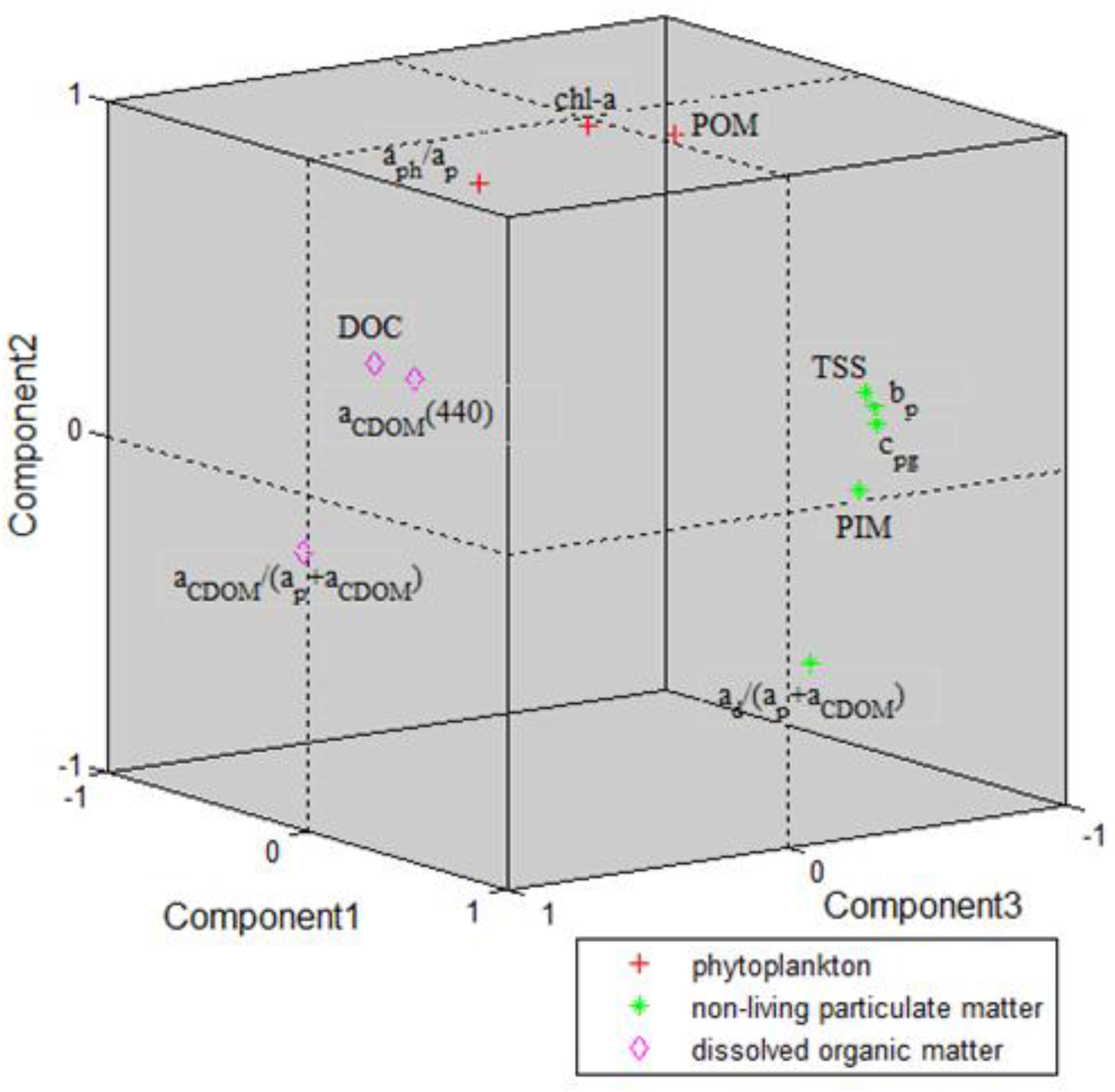
2.3. Factor Analysis of Environmental Parameters

Factor analysis was applied to test for correlation between variables, and to analyze whether several variables, such as chl-a, TSS, and a_CDOM (λ) could be replaced by common factors to represent optical water types. Of all 447 stations, 213 contained eleven variables (chl-a (mg·m⁻³), TSS (g·m⁻³), PIM (g·m⁻³), POM (g·m⁻³), DOC (g·m⁻³), a_CDOM (440) (m⁻¹), b_p (m⁻¹), c_pg (m⁻¹), a_CDOM/(a_p+ a_CDOM), a_d/(a_p + a_CDOM), and a_ph/a_p) and were analyzed. As explanation: a_CDOM (440) is a_CDOM (λ) at 440 nm; $b_p=\frac{{\displaystyle {\int }_{\lambda =400}^{750}{b}_p(\lambda )d\lambda }}{{\displaystyle {\int }_{\lambda =400}^{750}d\lambda }}$; $c_{pg}=\frac{{\displaystyle {\int }_{\lambda =400}^{750}{c}_{pg}(\lambda )d\lambda }}{{\displaystyle {\int }_{\lambda =400}^{750}d\lambda }}$; $a_{CDOM}/\left(a_p+a_{CDOM}\right)={\displaystyle \sum _{\lambda =400}^{750}{a}_{CDOM}(\lambda )}/({\displaystyle \sum _{\lambda =400}^{750}{a}_p(\lambda )}+{\displaystyle \sum _{\lambda =400}^{750}{a}_{CDOM}(\lambda )})$; $a_d/\left(a_p+a_{CDOM}\right)\text{=}{\displaystyle \underset{\lambda =400}{\overset{750}{\Sigma }}{a}_d(\lambda )}/({\displaystyle \underset{\lambda =400}{\overset{750}{\Sigma }}{a}_p(\lambda )}+{\displaystyle \underset{\lambda =400}{\overset{750}{\Sigma }}{a}_{CDOM}(\lambda )})$; $a_{ph}/a_p={\displaystyle \sum _{\lambda =400}^{750}{a}_{ph}(\lambda )}/{\displaystyle \sum _{\lambda =400}^{750}{a}_d(\lambda )}$.

Factor analysis was carried out as follows. First, the Kaiser-Meyer-Olkin (KMO) measure [53] and Bartlett’s sphericity test [54] were used to verify that these eleven variables were indeed suitable for factor analysis. Then, factor analysis, in which PCA was selected as the extraction method and varimax [55] as the rotation method, was implemented. Further, the excluded missing values option chosen was listwise—an option in which the entire observation is omitted from the analysis if any variable is missing.

2.4. Characteristic Wavelength Extraction

To reveal the implications of local peaks and troughs of the R_rs (λ) spectra of different classes, the characteristic wavelengths from the R_rs (λ) spectra were extracted. The extraction method was proposed by Lee et al. [56] and improved upon by Shen et al. [57], to distinguish effectively between the maximum and minimum values. A Savitzky-Golay filter [58,59] with a window size of 15 and a second-order polynomial was selected to smooth the R_rs (λ). The Savitzky-Golay filter can remove curves that have significant noise, while maintaining as much as possible the true shape of the original curve. Then, the first-order derivatives were calculated for each group, and f1_max (λ) and f1_min (λ) were used to represent the cumulative frequency at which the overall R_rs (λ) showed maximum and minimum values at a wavelength λ, respectively. The larger the f1_max (λ) or f1_min (λ), the greater was the probability of a maximum or minimum value appearing at λ.

3. Results and Discussion

FCM was used on all R_rs (λ) spectra to obtain final centroid sets corresponding to each Class i (i = 1, 2, 3, 4). To match the four centroid sets to types of optically complex waters, the environmental parameters associated with different R_rs (λ) spectra were assessed. Based on clustering results, a classification tree is provided as a supplement, and the feasibility of our centroids is estimated for several multispectral sensors.

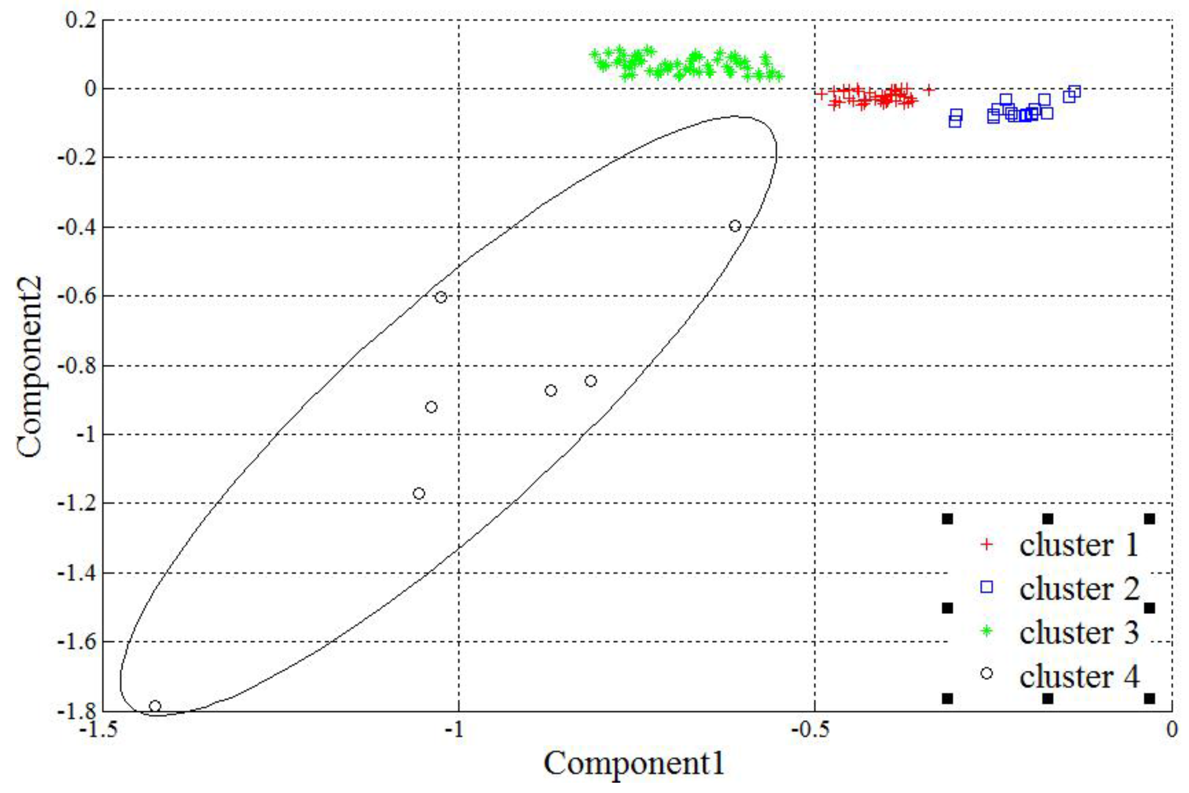
3.1. Clustering and Determination of Centroid Sets

The centroid sets are the basis for defining the membership of each pixel to each class. FCM was used to cluster R_rs (λ) spectra and obtain the centroid sets. To promote the robustness of FCM, the original R_rs (λ) data were strictly inspected prior to inclusion. Meanwhile, the classified spectra were inspected to determine whether certain classes contain very few samples that maybe outliers. Following such inspection, 447 stations were selected.

We ran the FCM routine on the 447 samples with values of c ranging from 2 to 15. Two validity measures were found to indicate the same number optimal number of clusters, c, which is four for our data set. Figure 3 shows the final results of the four clusters. Note that the seven samples in the ellipse of Figure 3 are far from the other samples. These seven samples were considered to be an independent Class 4, and the two validity measures run on the rest of data (Classes 1–3) again. The indices again implied these to be three clusters. The remaining data, except for Class 4, were then clustered into three clusters. The FCM routine was run on different similarity measures and the centroid sets were intersected. Of the 447 samples, 135 samples that were more representative than other samples were selected. The final four centroid sets covering 135 samples corresponding to Classes 1–4 are discussed in Section 3.2.

The test data set of 143 samples was used to extract the three centroid sets for Classes 1–3. The overall accuracy [60] and Kappa coefficient [61] were used to estimate the accuracy of the clustering method. The results prove that the accuracy of our methods with four similarity measures was better than the general FCM method with the Euclidean distance only. For the latter, the overall accuracy and Kappa coefficient was 89.7% and 0.844, respectively. The centroid sets corresponding to Classes 1–3 covered 16, 28, and 34 samples respectively. For the former, the overall accuracy was 100% (the respective overall accuracy for ED, SAD, OPD, TD was 89.2%, 100%, 100%, and 82.5%). Because the centroid sets intersected, some misclassified samples were removed. The three centroid sets corresponding to Classes 1–3 included 8, 28, and 26 samples, respectively.

Figure 3. The clustering results with four clusters. Component 1 and Component 2 are the first two principal components from Principal Component Analysis (PCA) of in situ R_rs (λ).

Figure 3. The clustering results with four clusters. Component 1 and Component 2 are the first two principal components from Principal Component Analysis (PCA) of in situ R_rs (λ).

The method presented here and the study by Moore et al. [1,24] are different in two aspects: (1) PCA transform is used before clustering in this work; (2) In the work of Moore et al., only Euclidean distance was used in FCM, whereas in our work, four different similarity distances—SAD, ED, OPD, and TD—were used and new centroid sets were extracted.

The three centroid vectors for each Class i (where i = 1, 2, 3) calculated from the four similarity measures were very similar to one another in shape (Figure 4). This demonstrates that the choice of similarity measure affected the centroids to a certain extent but did not drastically affect the final classification. This reflects the stability of the method presented here.

Figure 4. The clustering centroids when similarity measures are SAD, TD, OPD, and ED respectively.

Figure 4. The clustering centroids when similarity measures are SAD, TD, OPD, and ED respectively.

Normalization of R_rs [2,3,25], which could remove the differences in amplitudes rooted from gradients in concentrations, was recommended. However, we did not apply normalization here. Instead, we compared the mean reflectance spectra of the classes, derived from the (a) non-normalized (Classes 1, 2, 3, 4) and (b) normalized (Classes 1’, 2’, 3’,4’) in situ measurements, as shown in Figure 5. The mean spectra of classes with or without normalization yield similar distributions. In contrast, in Figure 3 in Vantrepotte et al. [2], the differences between classes in terms of spectral shape are lower when derived from the raw reflectance data than when derived from normalized spectra data.

Figure 5. Comparison of the mean reflectance spectra of the classes derived from (a) non-normalized (Classes 1, 2, 3, 4) and (b) normalized (Classes 1’, 2’, 3’, 4’) in situ measurements.

Figure 5. Comparison of the mean reflectance spectra of the classes derived from (a) non-normalized (Classes 1, 2, 3, 4) and (b) normalized (Classes 1’, 2’, 3’, 4’) in situ measurements.

Furthermore, we compared the average ±1 standard deviation of the raw reflectance spectra and the normalized reflectance spectra for the four classes (not shown). The variations within a class were slightly smaller in terms of normalized spectra than raw spectra, and did not differ significantly [3]. In summary, normalization has a minimal impact on our results. The reason may be the act of PCA transform before FCM. Normalization removed the differences in amplitude. The PCA transform preserved the main features of the spectra vectors, such as shape, which resulted in the FCM results not being predominantly influenced by the amplitude of the spectra.

3.2. Links Between R_rs (λ) Spectra and Environment Characteristics

Three steps were carried out to determine which types of optically complex waters the four centroid sets extracted by unsupervised classification represent. First, environmental parameters in each class were calculated. Secondly, differences between the R_rs (λ) among the four centroid sets were located. Then, these were paired to explain R_rs (λ) differences by essential IOPs knowledge and water quality parameters. All of the 135 samples selected in Section 3.1 were included.

(1)

Environment Characteristics of Each Group

Our results (Table 1) show that each optical class, defined by R_rs (λ) spectra, has unique environment characteristics.

Averages are shown in bold, with standard deviations in parentheses; minimum and maximum values are given in the square brackets. Minimums of all four classes are italicized, and maximums of all four classes are italicized and underlined. N is the number of samples.

Class 1 represents highly mixed eutrophic waters containing nonliving particulate matter, phytoplankton, and CDOM. In this class, the proportion of absorption of CDOM, phytoplankton, and nonliving particulate matter are about 20%, 20%, and 60%, respectively. For Class 1, the various parameters ranged between the maximum and minimum values of all classes, except for a_CDOM (440). The proportion of phytoplankton absorption was also found to only be lower than that of Class 4 and is higher than the average of the other three classes. Higher chl-a/TSS also indicates that the water is eutrophic. In addition, a_d/(a_p + a_CDOM) has a broader range, than the other classes. In other classes, the range of a_d/(a_p+ a_CDOM) is more limited.

Table 1. Overall and class-specific statistics for the bio-optical data collected during the cruises.

Parameter	All Classes	Class 1	Class 2	Class 3	Class 4
chl-a (mg·m−3)	44.2 (113.7)	41.8 (35.8)	7.8 (7.4)	15.1 (28.2)	429.0 (290.8)
	(0.0251–942.6)	(5.98–165.8)	(0.025–18.9)	(0.0391–152.5)	(149.8–942.6)
	N = 135	N = 44	N = 19	N = 65	N = 7
TSS (g·m−3)	95.6 (66.1)	48.9 (17.4)	12.3 (6.5)	150.6 (44.1)	105.0 (61.1)
	(3.75–244.9)	(21.5–91.1)	(3.75–26.6)	(55.2–244.9)	(32.6–213.9)
	N = 135	N = 44	N = 19	N = 65	N = 7
PIM (g·m−3)	78.1 (63.8)	34.8 (20.7)	8.29 (6.0)	133.7 (45.1)	24.3 (7.58)
	(0–222.5)	(4.1–81.5)	(0–22.0)	(7.9–222.5)	(13.0–35.7)
	N = 135	N = 44	N = 19	N = 65	N = 7
POM (g·m−3)	17.5 (20.9)	14.1 (9.8)	4.0 (1.8)	16.9 (6.4)	80.7 (57.7)
	(1.19–185)	(5.2–52.1)	(1.19–7.72)	(11.3–51.5)	(19.6–185.4)
	N = 135	N = 44	N = 19	N = 65	N = 7
DOC (g·m−3)	7.28 (2.03)	7.24 (1.20)	7.78 (2.28)	7.15 (2.49)	8.02 (0.65)
	(4.31–14.2)	(4.73–10.1)	(4.31–10.45)	(4.6–14.2)	(7.03–8.96)
	N = 135	N = 44	N = 19	N = 65	N = 7
aCDOM(440) (m−1)	0.87 (0.426)	0.98 (0.47)	0.96 (0.70)	0.76 (0.33)	0.95 (0.24)
	(0.290–2.40)	(0.35–2.40)	(0.29–2.36)	(0.33–2.14)	(0.68–1.42)
	N = 135	N = 44	N = 19	N = 65	N = 7
chl-a/TSS (10−3)	0.733 (1.14)	0.99 (0.847)	0.88 (1.21)	0.165 (0.46)	4.00 (0.77)
	(0.00089–5.01)	(0.098–3.60)	(0.00114–4.53)	(0.00089–2.30)	(2.96–5.01)
	N = 135	N = 44	N = 19	N = 65	N = 7
PIM/TSS	0.738 (0.239)	0.67 (0.234)	0.606 (0.246)	0.868 (0.13)	0.287 (0.123)
	(0–0.927)	(0.151–0.914)	(0–0.896)	(0.143–0.927)	(0.130–0.453)
	N = 135	N = 44	N = 19	N = 65	N = 7
POM/TSS	0.262 (0.239)	0.326 (0.234)	0.394 (0.246)	0.132 (0.131)	0.713 (0.123)
	(0.073–1.00)	(0.0857–0.849)	(0.104–1)	(0.073–0.857)	(0.547–0.870)
	N = 135	N = 44	N = 19	N = 65	N = 7
bp (m−1)	46.4 (29.0)	24.1 (8.11)	7.78 (2.34)	74.0 (12.7)	40.1 (32.5)
	(4.81–104.3)	(11.3–49.5)	(4.81–11.7)	(52.3–103.4)	(11.9–104.3)
	N = 85	N = 33	N = 7	N = 38	N = 7
cpg(m−1)	49.5 (30.7)	25.9 (8.35)	8.87 (2.19)	77.5 (13.2)	48.9 (41.7)
	(6.18–133.7)	(12.4–52.0)	(6.18–12.2)	(55.1–108.3)	(14.0–133.7)
	N = 85	N = 33	N = 7	N = 38	N = 7
aCDOM/(ap+ aCDOM)	0.157 (0.114)	0.194 (0.0642)	0.447 (0.065)	0.0848 (0.0319)	0.0850 (0.0819)
	(0.0110–0.540)	(0.0606–0.343)	(0.358–0.540)	(0.0225–0.163)	(0.0110–0.254)
	N = 85	N = 33	N = 7	N = 38	N = 7
ad/(ap+ aCDOM)	0.680 (0.235)	0.594 (0.157)	0.445 (0.0636)	0.883 (0.0408)	0.221 (0.124)
	(0.0943–0.960)	(0.201–0.874)	(0.394–0.556)	(0.7809–0.960)	(0.0943–0.380)
	N = 85	N = 33	N = 7	N = 38	N = 7
aph/ap	0.193 (0.239)	0.255 (0.206)	0.193 (0.0818)	0.0358 (0.0178)	0.748 (0.160)
	(0.0118–0.902)	(0.0495–0.778)	(0.114–0.314)	(0.0118–0.0752)	(0.519–0.902)
	N = 85	N = 33	N = 7	N = 38	N = 7

Table 1. Overall and class-specific statistics for the bio-optical data collected during the cruises.

Parameter	All Classes	Class 1	Class 2	Class 3	Class 4
chl-a (mg·m−3)	44.2 (113.7)	41.8 (35.8)	7.8 (7.4)	15.1 (28.2)	429.0 (290.8)
	(0.0251–942.6)	(5.98–165.8)	(0.025–18.9)	(0.0391–152.5)	(149.8–942.6)
	N = 135	N = 44	N = 19	N = 65	N = 7
TSS (g·m−3)	95.6 (66.1)	48.9 (17.4)	12.3 (6.5)	150.6 (44.1)	105.0 (61.1)
	(3.75–244.9)	(21.5–91.1)	(3.75–26.6)	(55.2–244.9)	(32.6–213.9)
	N = 135	N = 44	N = 19	N = 65	N = 7
PIM (g·m−3)	78.1 (63.8)	34.8 (20.7)	8.29 (6.0)	133.7 (45.1)	24.3 (7.58)
	(0–222.5)	(4.1–81.5)	(0–22.0)	(7.9–222.5)	(13.0–35.7)
	N = 135	N = 44	N = 19	N = 65	N = 7
POM (g·m−3)	17.5 (20.9)	14.1 (9.8)	4.0 (1.8)	16.9 (6.4)	80.7 (57.7)
	(1.19–185)	(5.2–52.1)	(1.19–7.72)	(11.3–51.5)	(19.6–185.4)
	N = 135	N = 44	N = 19	N = 65	N = 7
DOC (g·m−3)	7.28 (2.03)	7.24 (1.20)	7.78 (2.28)	7.15 (2.49)	8.02 (0.65)
	(4.31–14.2)	(4.73–10.1)	(4.31–10.45)	(4.6–14.2)	(7.03–8.96)
	N = 135	N = 44	N = 19	N = 65	N = 7
aCDOM(440) (m−1)	0.87 (0.426)	0.98 (0.47)	0.96 (0.70)	0.76 (0.33)	0.95 (0.24)
	(0.290–2.40)	(0.35–2.40)	(0.29–2.36)	(0.33–2.14)	(0.68–1.42)
	N = 135	N = 44	N = 19	N = 65	N = 7
chl-a/TSS (10−3)	0.733 (1.14)	0.99 (0.847)	0.88 (1.21)	0.165 (0.46)	4.00 (0.77)
	(0.00089–5.01)	(0.098–3.60)	(0.00114–4.53)	(0.00089–2.30)	(2.96–5.01)
	N = 135	N = 44	N = 19	N = 65	N = 7
PIM/TSS	0.738 (0.239)	0.67 (0.234)	0.606 (0.246)	0.868 (0.13)	0.287 (0.123)
	(0–0.927)	(0.151–0.914)	(0–0.896)	(0.143–0.927)	(0.130–0.453)
	N = 135	N = 44	N = 19	N = 65	N = 7
POM/TSS	0.262 (0.239)	0.326 (0.234)	0.394 (0.246)	0.132 (0.131)	0.713 (0.123)
	(0.073–1.00)	(0.0857–0.849)	(0.104–1)	(0.073–0.857)	(0.547–0.870)
	N = 135	N = 44	N = 19	N = 65	N = 7
bp (m−1)	46.4 (29.0)	24.1 (8.11)	7.78 (2.34)	74.0 (12.7)	40.1 (32.5)
	(4.81–104.3)	(11.3–49.5)	(4.81–11.7)	(52.3–103.4)	(11.9–104.3)
	N = 85	N = 33	N = 7	N = 38	N = 7
cpg(m−1)	49.5 (30.7)	25.9 (8.35)	8.87 (2.19)	77.5 (13.2)	48.9 (41.7)
	(6.18–133.7)	(12.4–52.0)	(6.18–12.2)	(55.1–108.3)	(14.0–133.7)
	N = 85	N = 33	N = 7	N = 38	N = 7
aCDOM/(ap+ aCDOM)	0.157 (0.114)	0.194 (0.0642)	0.447 (0.065)	0.0848 (0.0319)	0.0850 (0.0819)
	(0.0110–0.540)	(0.0606–0.343)	(0.358–0.540)	(0.0225–0.163)	(0.0110–0.254)
	N = 85	N = 33	N = 7	N = 38	N = 7
ad/(ap+ aCDOM)	0.680 (0.235)	0.594 (0.157)	0.445 (0.0636)	0.883 (0.0408)	0.221 (0.124)
	(0.0943–0.960)	(0.201–0.874)	(0.394–0.556)	(0.7809–0.960)	(0.0943–0.380)
	N = 85	N = 33	N = 7	N = 38	N = 7
aph/ap	0.193 (0.239)	0.255 (0.206)	0.193 (0.0818)	0.0358 (0.0178)	0.748 (0.160)
	(0.0118–0.902)	(0.0495–0.778)	(0.114–0.314)	(0.0118–0.0752)	(0.519–0.902)
	N = 85	N = 33	N = 7	N = 38	N = 7

Class 2 is comprised of relatively clear and CDOM-dominated water masses. Class 2 samples have the lowest average level of chl-a, TSS, PIM, POM, b_p, and c_pg of all classes (Table 1). Compared to the other classes, the a_CDOM/(a_p + a_CDOM) values are the highest, with an average of 0.447. CDOM may be generated by native production related to the bacterial activity that occurs during the phytoplankton biomass senescence phase. In addition, Class 2 has a high average absolute DOC concentration, of 7.78 g·m⁻³, which is higher than that of both Class 1 and Class 3. The relatively high average DOC values suggest that the particulate matter assemblage includes a relatively high proportion of detrital material from biodegradation.

Class 3 samples have extremely high levels of nonliving particulate matter. Most Class 3 samples are from windy lakes in spring or winter, and are affected by local sediment resuspension. Compared to the other classes, Class 3 has the highest levels of TSS, PIM, PIM/TSS, b_p, c_pg, and a_d/(a_p+ a_CDOM) (Table 1). In contrast, Class 3 has the lowest levels of DOC, a_CDOM (440), chl-a/TSS, POM/TSS, a_ph/a_p (Table 1).

Finally, Class 4 is comprised of seven samples collected during a heavy degree of cyanobacteria blooms. Although the number of Class 4 samples was low because there were few in situ measured samples, the seven samples are still representative of this class. Those R_rs are different from other classes, and represent the typical types of waters with a surface scum of cyanobacteria. Class 4 samples have extremely high concentrations of absolute chl-a and POM, and very high values of chl-a/TSS and POM/TSS ratios. The a_ph/a_p ratio of Class 4 is the highest of all four classes. In comparison, the PIM/TSS, a_d/(a_p + a_CDOM) and a_CDOM/(a_p + a_CDOM) ratios of Class 4 are far lower than those of the other classes.

To summarize, Classes 1–4 represent highly mixed eutrophic, CDOM-dominated relatively clear, nonliving solids-dominated and cyanobacteria-composed scum (or surface scum of cyanobacteria) water masses respectively.

In all 447 samples, chl-a varies from 0.0139 to 943 mg·m⁻³ (with an average of 34.5 mg·m⁻³). The maximal chl-a values correspond to heavy cyanobacteria blooms occurring annually in Lake Taihu between April and October. The TSS concentration ranges between 3.00 and 300 g·m⁻³, with an average value of 68.4 g·m⁻³. The range of a_CDOM (440) variation (0.138–4.79 m⁻¹, with an average of 0.83 m⁻¹) covers a large fraction of the natural variability reported in high contrast areas. The dataset of 447 samples considered in this work spans four orders of magnitude in chl-a concentration and two orders of magnitude in TSS, PIM, and POM concentrations, and b_p and c_pg. The four water types determined here should be therefore be broadly representative.

Table 2. Numbers of in situ data distributed across the four classes.

Class	Lake Chaohu	Three Gorges Reservoir	Lake Dianchi	Yellow River Estuary	Lake Taihu (Spring)	Lake Taihu (Summer)	Lake Taihu (Autumn)	Lake Taihu (Winter)	Total
1	21	2	24	4	67	39	31	44	232
2	0	4	1	43	7	3	6	5	69
3	8	16	6	7	51	1	3	47	139
4	0	0	0	0	6	1	0	0	7
Total	29	22	31	54	131	44	40	96	447

Table 2. Numbers of in situ data distributed across the four classes.

Class	Lake Chaohu	Three Gorges Reservoir	Lake Dianchi	Yellow River Estuary	Lake Taihu (Spring)	Lake Taihu (Summer)	Lake Taihu (Autumn)	Lake Taihu (Winter)	Total
1	21	2	24	4	67	39	31	44	232
2	0	4	1	43	7	3	6	5	69
3	8	16	6	7	51	1	3	47	139
4	0	0	0	0	6	1	0	0	7
Total	29	22	31	54	131	44	40	96	447

Environmental conditions, governed by the water constituents and the optical properties of the water column, are not unique to any particular lake, reservoir, or coastal area. Table 2 shows the distribution of data from each site across the four classes. The distributions of data for each class span multiple water types, with freshwater and marine stations found in the same class. This demonstrates the limitations of regional inversion algorithms, which are temporally and spatially dependent, as well as the advantages of approaches based on classification.

In this study, several environmental parameters were considered, including water constituents (e.g., phytoplankton and nonliving particulate matter) and optical properties of the water column (e.g., b_p, a_ph, a_p, a_CDOM). To examine the potential relationships among such parameters, factor analysis—a statistical method used to describe variability among observed variables in terms of a lower number of unobserved variables—was applied to the 447 samples (Figure 6). Figure 6 shows that chl-a, POM and a_ph/a_p are similar in nature and close to 1 at the Component 2 axis. TSS, PIM, b_p, c_pg and a_d/(a_p + a_CDOM) are clustered near 1 at the Component 1 axis. DOC, a_CDOM (440), and a_CDOM/(a_p+ a_CDOM) are grouped with large values at the Component 3 axis. It can be inferred that the three components represent nonliving particulate matter, phytoplankton, and dissolved matter of biological origin (both living and detrital) respectively. Among the 11 components, only three components’ eigenvalues are larger than one. The cumulative percentage of the first three components reaches 89.32%, explaining the majority of the total variance. The rotated factor loadings represent how the variables are weighted for each factor. The parameters b_p and c_pg contribute more to Component 1 than do TSS and PIM. a_CDOM (440) contributes more to Component 3 than does DOC, and a_ph/a_p contributes less to Component 2 than do chl-a and POM. In general, the IOPs contribute to the components as much as the water quality parameters do. The above correlated parameters, including water quality parameters and IOPs, can be replaced by three potential components, nonliving particulate matter, phytoplankton, and CDOM, which are precisely the three main optically active substances in waters [62].

Figure 6. Component plot in rotated space.

Figure 6. Component plot in rotated space.

(2)

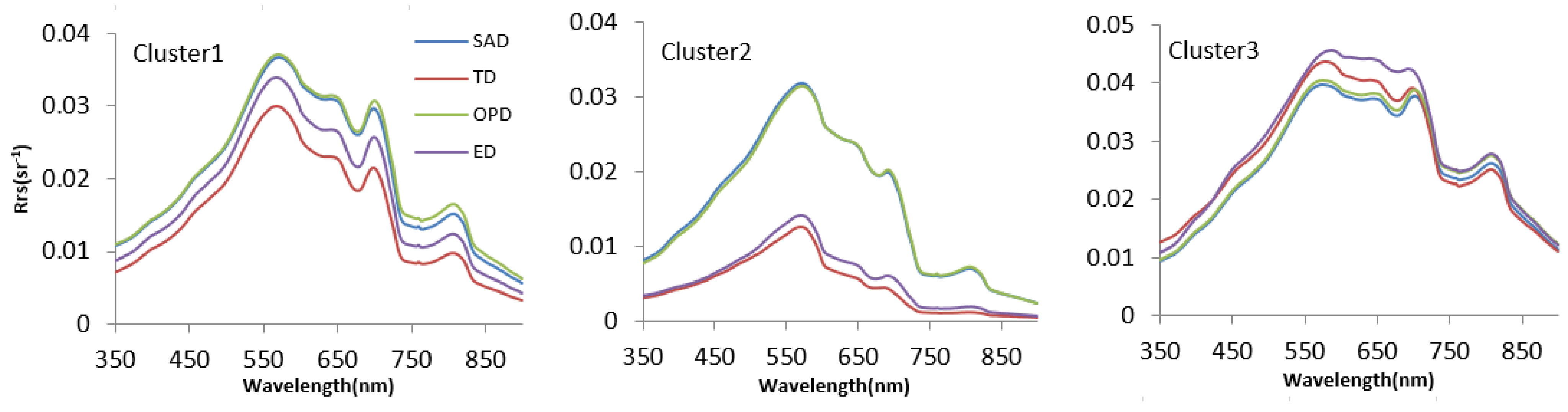
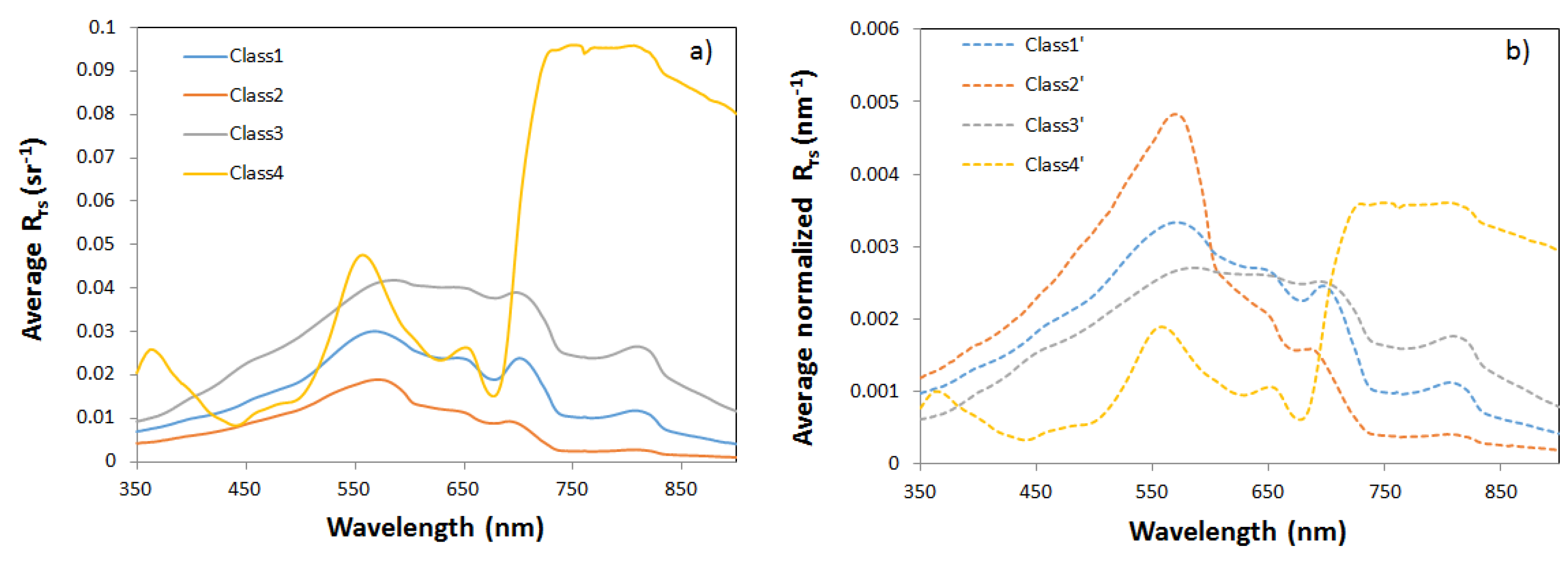
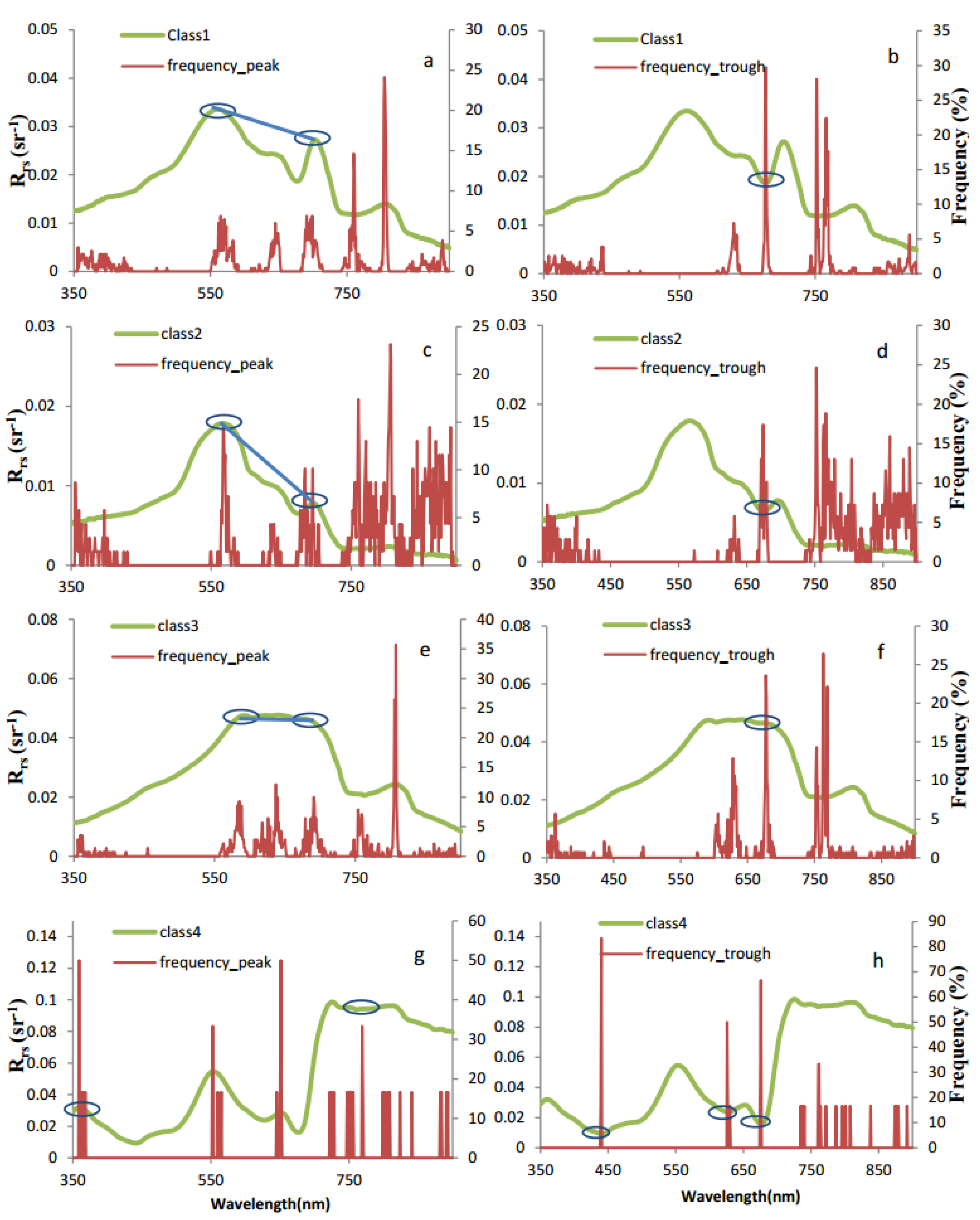
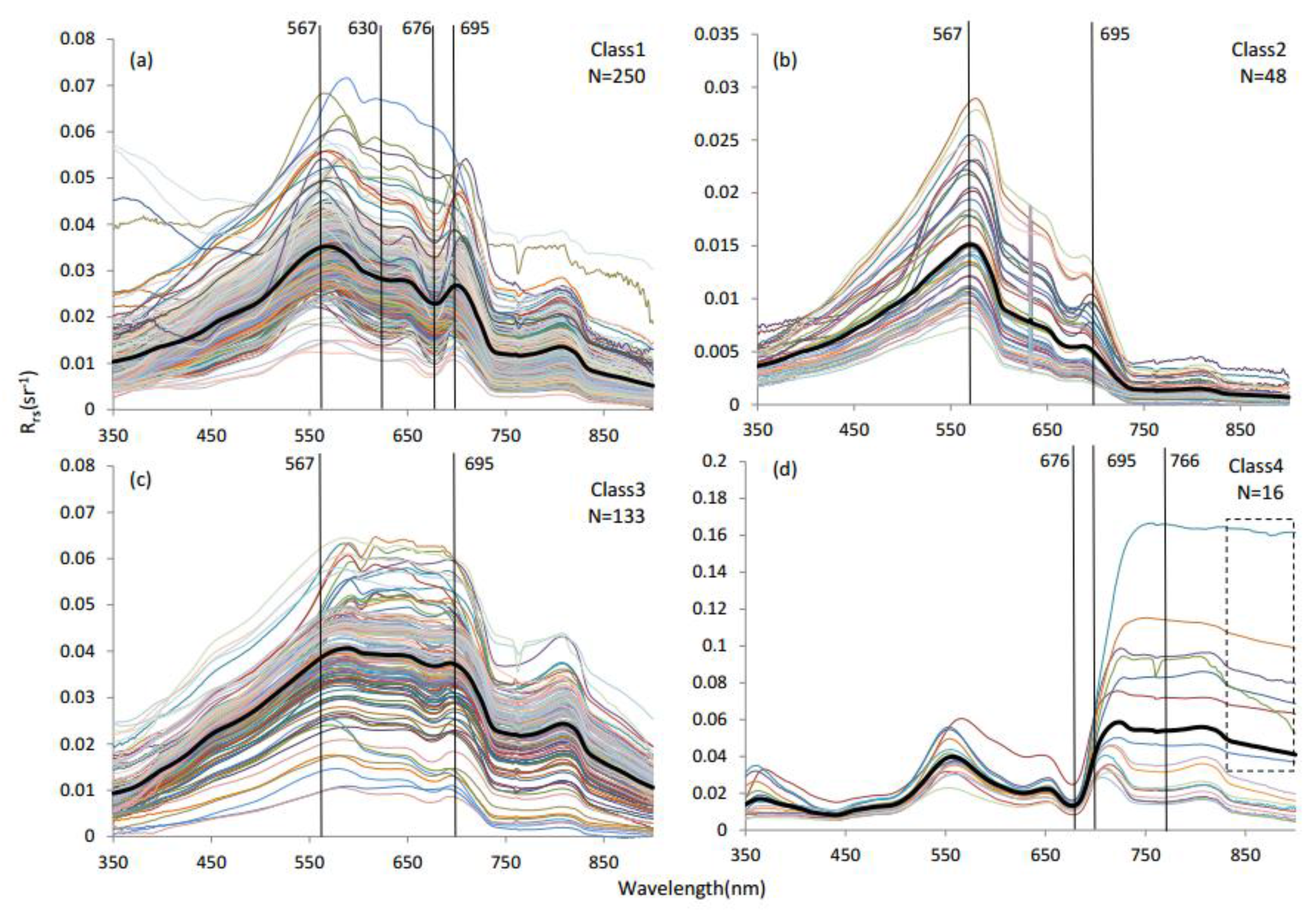
Characteristics of R_rs (λ) Spectra and correspondence with environmental parameters

The link between R_rs (λ) and environmental parameters has a theoretical basis. The concentrations and constitutes of organic and inorganic particulate and dissolved matter impact the absorption and scattering of light. The IOPs (including absorption and backscattering coefficients), as well as illumination and viewing geometries, jointly determine R_rs (λ). In other words, optically complex waters that have similar environment conditions can be expected to have apparent reflectance spectra with similar shapes [63]. Here, we provide some implications of the local peaks and troughs of the spectral curves of each class, aiming to both reveal the relationships between R_rs (λ) spectra and environment conditions as well as to achieve a simplified representation of R_rs (λ).

The wavelength distributions of f1_max (λ) and f1_min (λ) were obtained as the “frequency_peaks” and “frequency_troughs” for the four different classes (Figure 7). The frequency diagrams show a correspondence between the local frequency maxima and the extreme points (maxima and minima) of the average spectral curves in each centroid set.

The spectral curves also exhibit different characteristics in each of the four classes. On the basis of field experience, Class 4 is unique, representing waters with a surface scum of cyanobacteria bloom. The distinctly high values in the near-infrared spectral range result from the backscattering of the algae, which far outweigh the absorption of pure water. A reflection peak at around 359 nm in Class 4 is caused by a local absorption minimum, which is formed by the coinciding negative exponential decrease of a_d + a_CDOM and an increase in a_ph at wavelengths of approximately 300–400 nm. Chl-a absorption around 440 nm caused the narrow reflection troughs near 439–440nm in Class 4.

For Class 1 to Class 3, five characteristic wavelengths were observed, which can be used to discriminate optical types: peaks around 567–585 nm, 637–651 nm and 684–695 nm, and troughs around 626–632 nm and 674–677 nm. The five features listed above are mainly affected by pigment absorption, and also by the integrated absorption or scattering of pure water, nonliving particles, phytoplankton, and CDOM in each optical class.

The central positions of the trough near 674–677 nm and of the peaks near 637–651 nm and 684–695 nm are due to the absorption of chl-a. Class 4 and Class 1 have relatively higher chl-a concentrations in comparison with the low chl-a concentration waters of Class 2 and Class 3. The peaks near 560–580 nm shift to longer wavelengths when TSS concentrations increase as long as there is no algae bloom. In Class 3 samples, TSS is high and dominates; the central position of the peak is 585 nm, ranging from 560–596 nm. In contrast, Class 1 and Class 2 samples are from waters with lower TSS; the central position of the peak is consistently at 567 nm. The peaks near 684–695 nm all have a large range of variation for the four classes. The peak in Class 3 samples shifts to 695 nm, demonstrating that it does not matter whether TSS or chl-a dominates, the peak will be found at a longer wavelength as long as chl-a concentration is high.

Note that there is an obvious broad, flat peak between 560–695 nm in Class 3 samples. Class 2 samples show a peak at around 567 nm and a decreasing slope between 567 nm and 690 nm. Class 2 is comprised of CDOM-dominated water masses, with about 45% a_CDOM/(a_p + a_CDOM). Class 1 samples fall between Classes 3 and 2, representing highly mixed eutrophic waters, with two obvious peaks at around 567 nm and 695 nm.

To summarize, the characteristics of the R_rs (λ) spectra correspond with the measured water quality parameters and optical properties. They could be matched up well in each class. It is also partially indicated that the R_rs (λ) spectra of the resulting centroid sets are representative and reasonable.

Figure 7. The R_rs (λ) of the four class centroids and the corresponding frequency distributions of the peaks and troughs. Blue circles mark the positions of the main peaks and troughs of interest. (a): class 1 centroid; (b): the frequency distributions of class 1; (c): class 2; (d): the frequency distributions of class 2; (e): class 3; (f): the frequency distributions of class 3; (g): class 4; (h): the frequency distributions of class 4.

Figure 7. The R_rs (λ) of the four class centroids and the corresponding frequency distributions of the peaks and troughs. Blue circles mark the positions of the main peaks and troughs of interest. (a): class 1 centroid; (b): the frequency distributions of class 1; (c): class 2; (d): the frequency distributions of class 2; (e): class 3; (f): the frequency distributions of class 3; (g): class 4; (h): the frequency distributions of class 4.

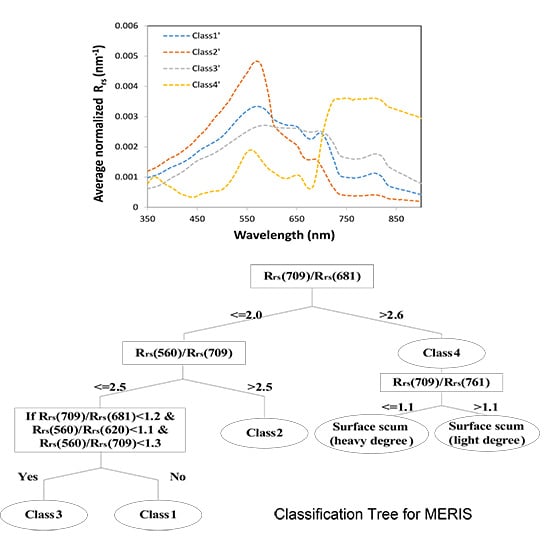
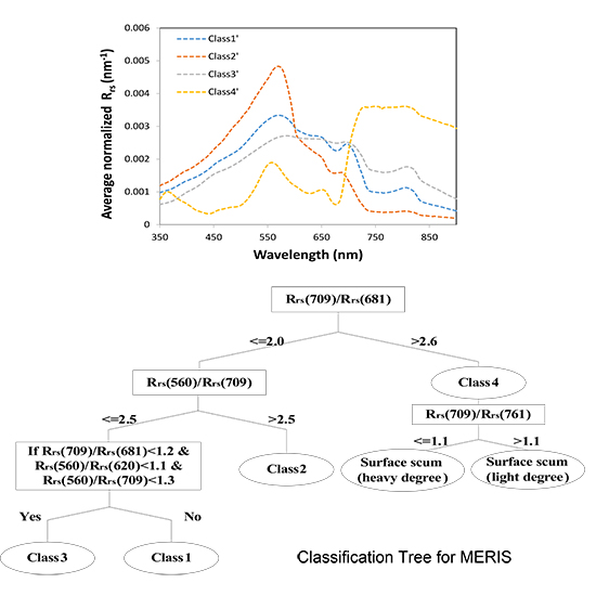
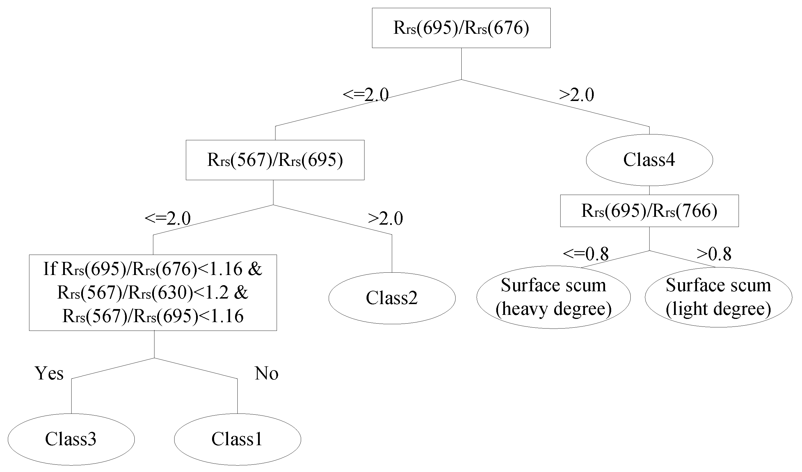
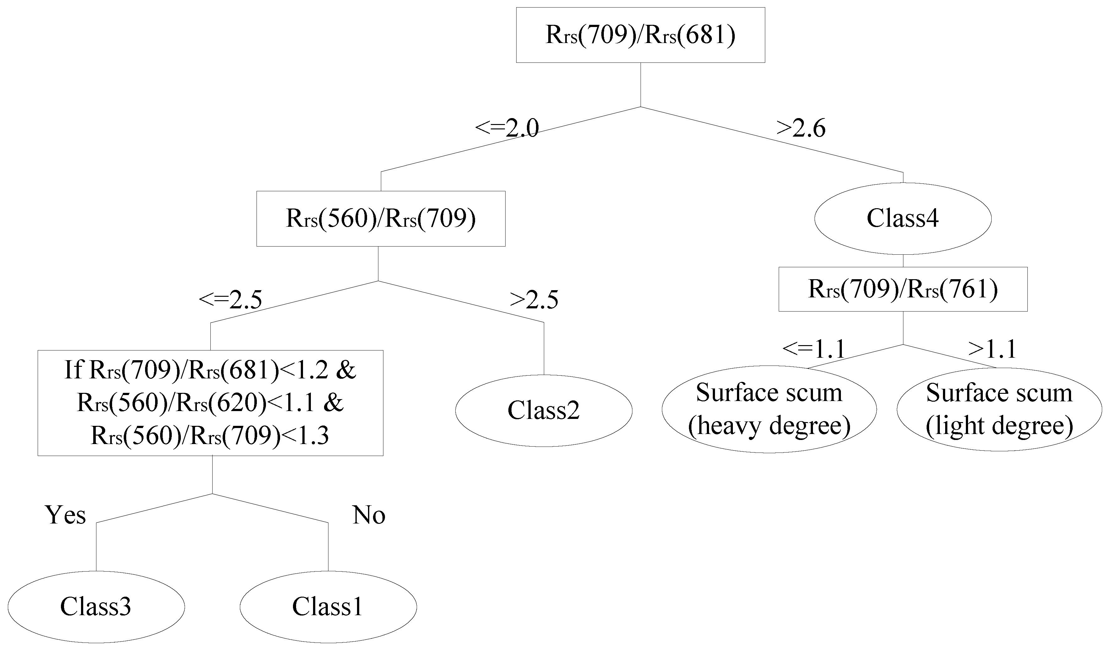
3.3. Classification Tree

Centroids can be used in both fuzzy and hard classification. However, a classification tree can only be used in hard or strict classification. The results of the former are more practical than the latter. However, the operational efficiency of the latter is higher than that of the former. To supplement a classification method and to make the most of the given R_rs (λ) features, an classification tree is provided here.

According to the characteristic wavelengths described in the preceding section, R_rs (567), R_rs (630), R_rs (645), R_rs (676), and R_rs (695) are recommended to classify the four optical water types found here. Band ratios are often used as a classification feature as it can eliminate environmental effects. Five bands are combined pair-wise into 10 combination ratios: R_rs (567)/R_rs (630), R_rs (567)/R_rs (695), R_rs (695)/R_rs (676), R_rs (695)/R_rs (766), R_rs (695)/R_rs (630), R_rs (567)/R_rs (676), R_rs (567)/R_rs (766), R_rs (676)/R_rs (766), R_rs (630)/R_rs (676), and R_rs (630)/R_rs (766).

To make the classification tree more applicable, we also expanded our sample size. In addition to the 135 classified samples, the remaining 312 samples were grouped into the given classes by a maximum of four grades of membership. The ranges of the above 10 ratios were calculated for the samples belonging to each of the four classes. Then, some of the ratios and thresholds were found to distinguish any two classes very well, in spite of individual exceptions. For example, R_rs (695)/R_rs (676) ranged 0.76–1.23 for Class 3, except that the ratio of one sample was 2.39. The ratio ranged 2.13–3.32 for Class 4. Thus, the sample in Class 3 had to be moved into Class 4 when the ratio R_rs (695)/R_rs (676) was chosen as a classification feature, and the threshold was 2.0. Then, the range of a certain ratio in a given class would not overlap with any other class. After slight adjustment, a new set of classifications was formed (Figure 8). Class 1 contained 250 samples, and Class 2 to Class 4 contained 48, 133, and 16 samples, respectively.

Figure 8. The adjusted classification based on the extended dataset, with the centroids in bold ((a): class 1; (b): class 2; (c): class 3; (d): class 4). The dashed rectangle in Class 4 includes seven samples from a heavy surface scum composed of cyanobacteria blooms. Black bars mark the discussed wavelengths.

Figure 8. The adjusted classification based on the extended dataset, with the centroids in bold ((a): class 1; (b): class 2; (c): class 3; (d): class 4). The dashed rectangle in Class 4 includes seven samples from a heavy surface scum composed of cyanobacteria blooms. Black bars mark the discussed wavelengths.

Among the four classes, Class 4 samples could be easily distinguished due to the obvious high values at near-infrared wavelengths, which resulted from the backscattering of the algae. The ratio of R_rs (695)/R_rs (676) can therefore be used to distinguish Class 4. This ratio ranges 0.91–1.98, 0.85–1.23, and 0.94–1.16 for Classes 1–3, respectively. Thus the threshold to distinguish Class 4 is selected as 2.0, since the ratio ranges 2.13–3.32 for the 16 samples in Class 4.

In Class 4, based on in situ observations, the samples corresponding to light degrees of surface scum have lower values at near-infrared wavelengths than those that correspond to heavy degrees of surface scum. As shown in the dashed rectangle in Figure 8, the R_rs (695)/R_rs (766) ratios of these nine samples, ranging 0.89–1.64, are obviously higher than those of the seven samples (0.29–0.74) corresponding to heavy degrees of surface scum. The heavy surface scum samples can therefore be distinguished when the R_rs (695)/R_rs (766) value is less than 0.8. In addition, the eutrophic Class 1 samples, which contained the highest number of samples of all classes, can be divided according to chl-a concentration levels using R_rs (695)/R_rs (766).

Class 2 samples tend to be easily distinguished by a spike near 567 nm, and a steep decline following the spike. A R_rs (567)/R_rs (695) value, usually known as the green/red ratio, can therefore be utilized to distinguish Class 2 from the other classes. The range of R_rs (567)/R_rs (695) in Class 2 samples is 2.01–4.76, compared with 1.03–1.96 in Class 1 and 0.82–1.91 in Class 3. The weaker decline between 567 nm and 695 nm in Class 1 or Class 3 is due to strong backscattering at the corresponding range in relatively turbid waters.

Class 3 and Class 1 are relatively difficult to distinguish. The following are the essential differences between Class 1 and Class 3: Class 3 is dominated by nonliving particulate matter with no obvious pigment absorption characteristics, while Class 1 is also significantly affected by phytoplankton, with obvious spectral characteristics at around 630 nm and 676 nm. Thus, R_rs (695)/R_rs (676), which is positively correlated with chl-a [64,65,66], and R_rs (630), which is related to phycocyanin [45,67], are selected as indices. Also note that the R_rs (λ) spectra in Class 3 are typically flat between 560 and 695 nm. In contrast, the R_rs (λ) spectra in Class 1 decrease from 560 nm to 695 nm. Low ratios of R_rs (567)/R_rs (695) are therefore chosen together as additional criteria to identify Class 3. When the R_rs (695)/R_rs (676) < 1.16 and R_rs (567)/R_rs (630) < 1.2, 78 Class 1 samples were misclassified into Class 3. Combined with the R_rs (567)/R_rs (695) index, these 78 misclassified samples of Class 1 were completely separated from the 133 Class 3 samples.

Figure 9. Classification tree for dividing waters applied to hyperspectral R_rs (λ) images.

Figure 9. Classification tree for dividing waters applied to hyperspectral R_rs (λ) images.

In summary, the five ratios consisting of 567 nm, 630 nm, 676 nm, and 695 nm were primarily used to identify Classes 1–4. A classification tree for several optically complex waters in China was proposed based on hyperspectral R_rs (λ) images. The structure of the dendrogram is shown in Figure 9. The classification tree was tested using a test data set comprising 143 samples. The overall accuracy was 79.7% and the Kappa coefficient was 0.697.

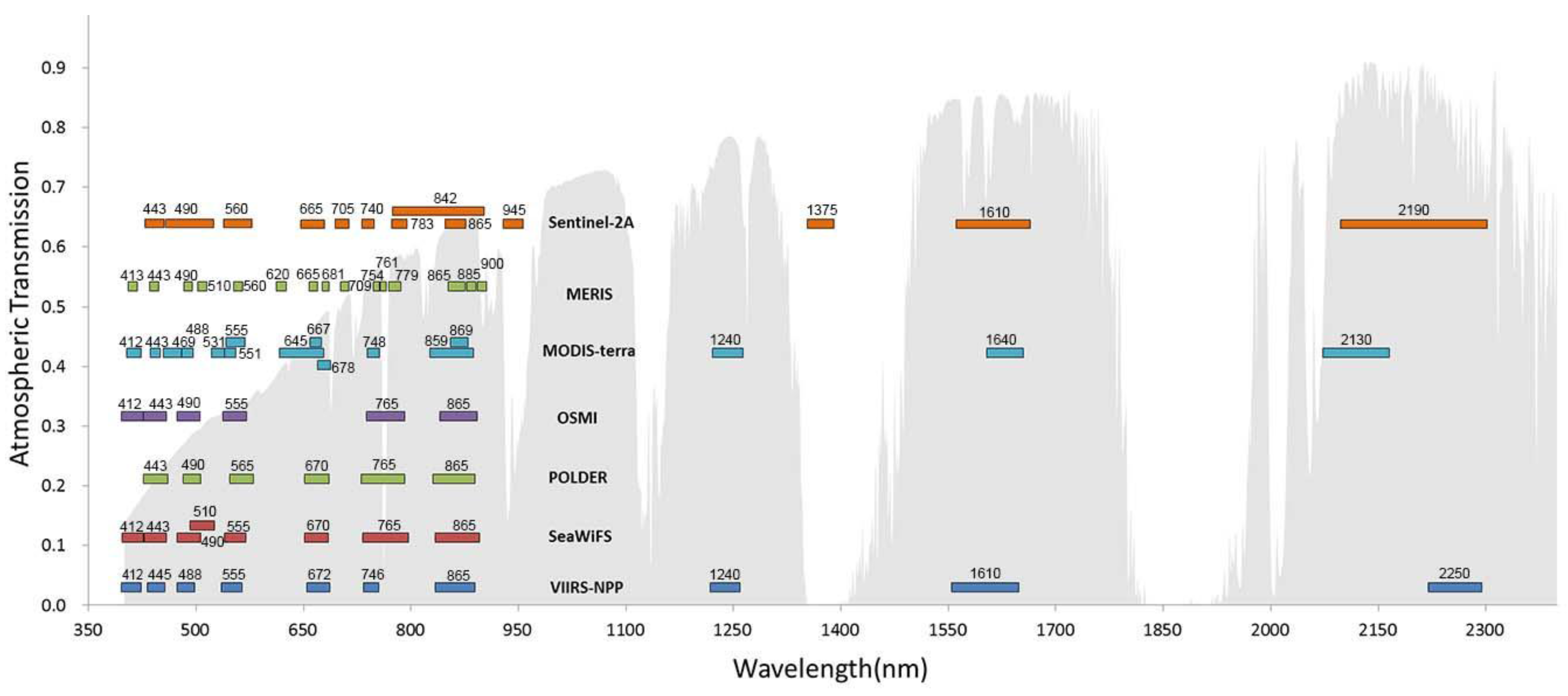
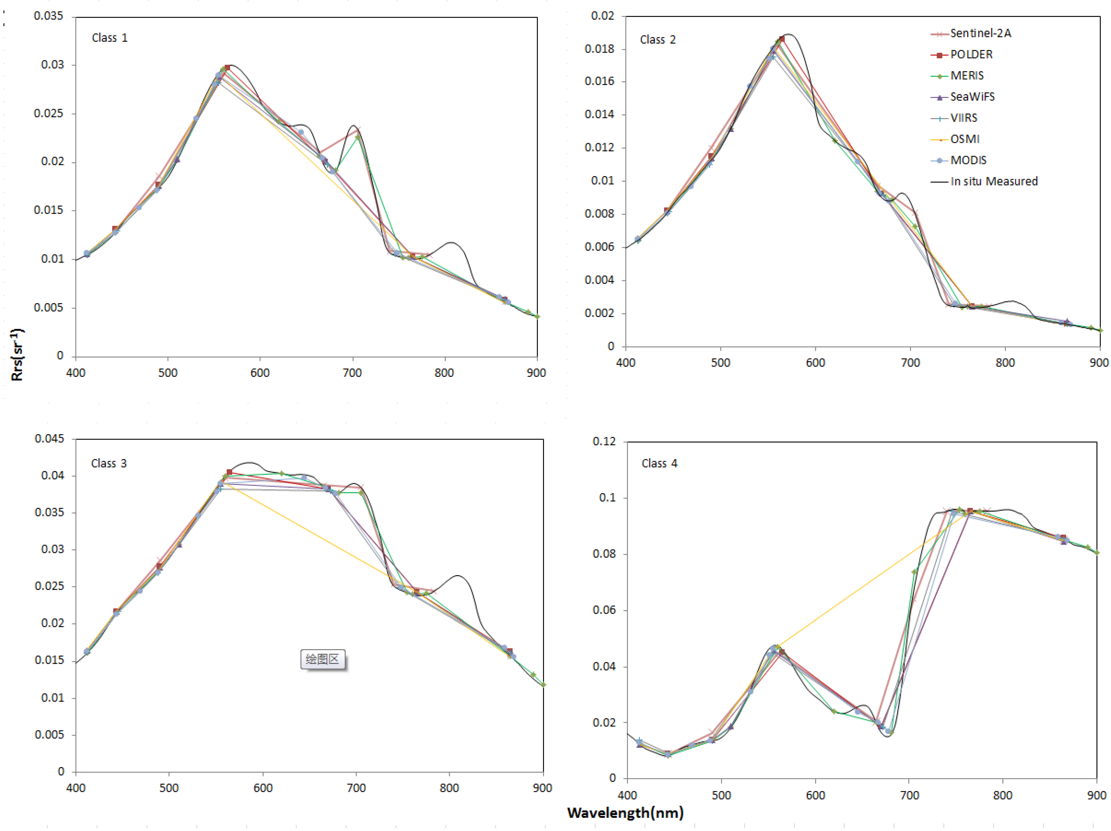
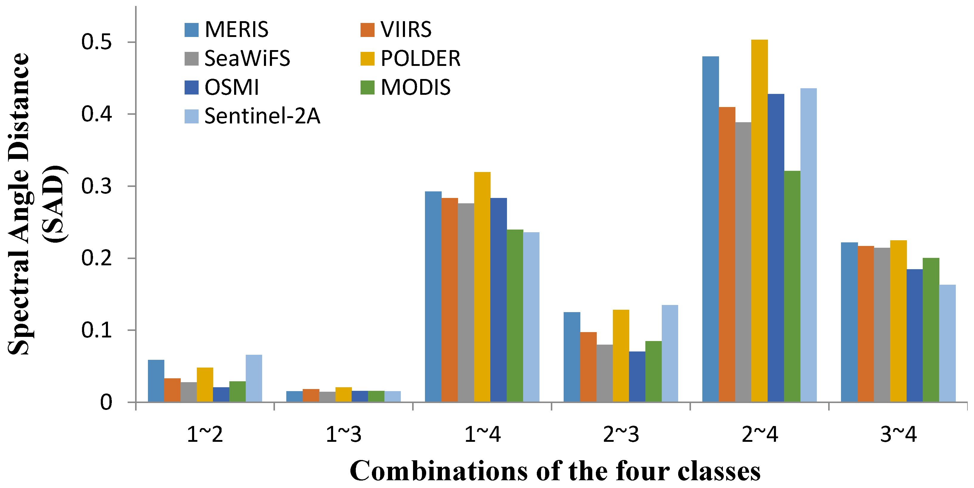
3.4. Reflectance Discrimination Using Ocean Color Satellite Sensors

For hyperspectral remote sensors, such as Hyperion, equipped with hundreds of continuous spectral bands, it is no problem to apply the classification scheme proposed in this study because the centroids provided are from continuous spectra and the band ratios require several narrow bands. However, for multispectral sensors, bands generally do not cover the full spectrum, only a discrete section, and band width is usually greater than 10 nm. Some subtle characteristics may therefore be missed or obscured by the coarser resolution sensors. The feasibility of using our centroids with data from multispectral sensors should therefore be assessed. Seven sensors commonly used in ocean color, including Sentinel-2A, MEdium Resolution Imaging Spectrometer (MERIS), the Visible Infrared Imager Radiometer Suite (VIIRS) onboard earth-observing satellite NPP, Sea-Viewing Wide Field-of-View Sensor (SeaWiFS), POLarization and Directionality of the Earth's Reflectances (POLDER), Ocean Scanning Multispectral Imager (OSMI), and MODerate-resolution Imaging Spectroradiometer (MODIS), were analyzed. Here, the relative spectral responses of POLDER-1 and MODIS-Terra were selected to represent POLDER and MODIS.

The ground sample distances of the seven sensors are approximately 0.2 km, 0.3 km (full resolution), 0.4 km (subastral point), 1.1 km (local area coverage), 6 km, 0.85 km, and 1 km respectively. Figure 10 shows the band placements of the seven selected sensors.

Figure 10. Band placement and width specifications of the seven satellite sensors selected. The atmospheric transmission of the y-axis is associated with grey curves, but not with the vertical placement of the difference sensors.

Figure 10. Band placement and width specifications of the seven satellite sensors selected. The atmospheric transmission of the y-axis is associated with grey curves, but not with the vertical placement of the difference sensors.

If the R_rs spectra acquired from satellite images covering four types of waters have significant differences, the satellite sensor can be viewed as suitable to classify the several optical complex waters in China. The average in situ R_rs (λ) of each centroid set was first calculated to obtain the R_rs (λ) centroids associated with four optical types. The R_rs (λ) was then convolved with solar irradiance and the relative spectral response (RSR) from each of the ocean color remote sensors. Figure 11 compares the centroids from the in situ measured spectra and those simulated by the seven ocean color satellite sensors. Figure 11 shows that the spectrum of a given sample has a similar shape when observed by six of the sensors: Sentinel-2A, MERIS, VIIRS, SeaWiFS, POLDER, and MODIS. However, OSMI does not have a band near 670 nm, and therefore misses the trough there. In general, the spectra of the Class 4 optical water type are the most unique because they represent a surface scum composed of cyanobacteria blooms. The spectra of the other three optical water types have some differences, however it is difficult to interpret such differences qualitatively from Figure 11.

Figure 11. In situ measured centroid spectra and those simulated by seven ocean color satellite sensors for the four optical water types. The seven ocean color satellite sensors are Sentinel-2A, MERIS, VIIRS, SeaWiFS, POLDER, OSMI, and MODIS.

Figure 11. In situ measured centroid spectra and those simulated by seven ocean color satellite sensors for the four optical water types. The seven ocean color satellite sensors are Sentinel-2A, MERIS, VIIRS, SeaWiFS, POLDER, OSMI, and MODIS.

To quantitatively assess the discriminability of the four centroids by the commonly used satellite sensors, the SADs between any two centroids was calculated, as shown in Figure 12. In general, the seven sensors were all found to effectively discriminate Class 4 from the other classes, and the SAD values between Classes 1 and 4, Classes 2 and 4, and Classes 3 and 4 almost exceeded 0.2. The SAD values were also able to differentiate between Class 2 and Class 3. However, it is difficult for them to discriminate Class 1 from Class 2, and Class 1 from Class 3. POLDER is the sensor best able to distinguish between the four water types, followed by MERIS. Sentinel-2A ranks the third in general. Except for Class 4, Sentinel-2A is the sensor best to distinguish between Classes 1–3. To summarize, Sentinel-2A (with a better spatial resolution), MERIS, and POLDER are the best choices for discriminating between the four optical water types. The performance of VIIRS, SeaWiFS, MODIS, and OSMI in this respect was found to decrease successively.

Figure 12. The six spectral angle distance (SAD) combinations produced by any two classes, the centroids of which have been simulated for the seven satellite sensors. The y-axis shows the SAD, which has a value of between 0 and 1. The x-axis shows the six combinations of the four classes. For each combination, the seven color bars denote the SADs of Sentinel-2A-, MERIS-, VIIRS-, SeaWiFS-, POLDER-, OSMI-, and MODIS-measured spectra.

Figure 12. The six spectral angle distance (SAD) combinations produced by any two classes, the centroids of which have been simulated for the seven satellite sensors. The y-axis shows the SAD, which has a value of between 0 and 1. The x-axis shows the six combinations of the four classes. For each combination, the seven color bars denote the SADs of Sentinel-2A-, MERIS-, VIIRS-, SeaWiFS-, POLDER-, OSMI-, and MODIS-measured spectra.

Figure 13. Classification tree for dividing waters applied to MERIS.

Figure 13. Classification tree for dividing waters applied to MERIS.

Further, a classification tree was built based on 447 training samples simulated by the MERIS sensor, as shown in Figure 13. MERIS bands 5, 6, 8, 9, and 11—with central wavelengths at 560 nm, 620 nm, 681 nm, 709 nm, and 761 nm, respectively—were utilized. The classification tree was tested using the test data set comprising 143 samples. The overall accuracy was 76.2% and the Kappa coefficient was 0.632. The advantage of the classification tree is that it does not use some of the MERIS blue bands, such as 413 nm, 443 nm, and 490 nm, which have large errors caused by atmospheric correction. The characteristics at these wavelengths are obvious in clear waters, but not in our samples, as shown in Figure 8. The disadvantage is that the misclassification rate in Class 1 is 33.3%, which is marginally high. This is because Class 1 is a mixed class, and not as pure as Classes 2–4. In the future, Class 1 will be further broken down into subclasses.

4. Summary and Conclusions

This study presents an improved FCM method to classify optically complex waters using R_rs (λ), over a broad range of water quality parameters. We provide a set of centroids from in situ R_rs (λ) presenting typical optical types by the fuzzy clustering method. Then we use IOPs and water quality parameters to provide evidence for which type of waters each cluster represents. The process reduces subjectivity and has interpretation of physical mechanism. A classification tree is also provided as a supplement.

Four robust R_rs (λ) centroid sets consisting of 135 stations resulted from plugging different similarity measures into FCM clustering (from a total of 447 stations). The accuracy of our methods with four similarity measures (overall accuracy: 100%) was better than that of the general FCM method with Euclidean distance only (overall accuracy: 89.7%). Normalization of R_rs, which was recommended to remove the differences in amplitudes rooted from gradients in concentrations, had minimal impact on our results. This minimal impact may be because PCA transform was performed before FCM.

Four R_rs (λ) vectors express the four types of optically complex waters: (1) Highly mixed eutrophic waters, with the proportion of absorption of CDOM, phytoplankton, and non-living particulate matter at approximately 20%, 20%, and 60% respectively; (2) CDOM-dominated relatively clear waters, with approximately 45% a_CDOM/(a_p + a_CDOM); (3) nonliving solids-dominated waters, with approximately 88% a_d/(a_p + a_CDOM); and (4) cyanobacteria-composed scum. Our investigated samples are from typical optically complex waters from around China, spanning both freshwater and estuarine environments. Local peak and trough features of the R_rs (λ) centroid sets were located and statistical analysis was performed on several environmental parameters of each class. In Class 3 samples, a distinct broad, flat peak is found between 560 and 695 nm. Class 2 samples show a peak around 567 nm and a decreasing slope between 567 and 690 nm. Class 1 samples fall between Class 3 and Class 2, with two obvious peaks around 567 and 695 nm. Class 4 samples have distinct high values at near-infrared wavelengths. The R_rs (λ) features of the different classes were found to correspond to values of IOPs and water quality parameters.

A classification tree that integrates the characteristics of R_rs (567)/R_rs (630), R_rs (567)/R_rs (695), R_rs (695)/R_rs (676), and R_rs (695)/R_rs (766) was proposed for hyperspectral sensors based on analysis of the characteristics of R_rs (λ). The discrimination ability for the given optical water types using simulated spectral measurements from seven multispectral sensors was also investigated. For the four optical water types, POLDER, Sentinel-2A, and MERIS have the strongest discrimination performance, followed by the performance of VIIRS, SeaWiFS, MODIS, and OSMI in decreasing order. A classification tree for MERIS was also proposed. The overall accuracy and Kappa coefficient were 76.2% and 0.632, respectively.

This method, which is based on various similarity measures, is better than the general FCM method, which uses Euclidean distance only. The method is found to enhance the representativeness and robustness of the resulting centroids, which can be applied in other studies to classify optical water types. By comparing the observed R_rs (λ) with the known typical spectra, the class which each pixel belongs to can be determined. Via classification, knowledge of which substance (e.g., nonliving solids, CDOM, and phytoplankton) dominates in different types of waters can be obtained. The final centroid sets could also be used in a class-based inversion approach to retrieve the concentrations of water constitutes using remote sensing images, using the classification memberships as weights. In addition, the four water types proposed in this paper are not only suitable for the application of hyperspectral remote sensing but also appropriate for multispectral sensor-based classification.

References

1. Moore, T.S.; Dowell, M.D.; Bradt, S.; Ruiz Verdu, A. An optical water type framework for selecting and blending retrievals from bio-optical algorithms in lakes and coastal waters. Remote Sens. Environ. 2014, 143, 97–111. [Google Scholar] [CrossRef] [PubMed]
2. Vantrepotte, V.; Loisel, H.; Dessailly, D.; Mériaux, X. Optical classification of contrasted coastal waters. Remote Sens. Environ. 2012, 123, 306–323. [Google Scholar] [CrossRef]
3. Vantrepotte, V.; Mélin, F. How optically diverse is the coastal ocean? Remote Sens. Environ. 2015, 160, 235–251. [Google Scholar] [CrossRef]
4. Zhang, Y.; Feng, L.; Li, J.; Luo, L.; Yin, Y.; Liu, M.; Li, Y. Seasonal–spatial variation and remote sensing of phytoplankton absorption in Lake Taihu, a large eutrophic and shallow lake in China. J. Plankton. Res. 2010, 32, 1023–1037. [Google Scholar] [CrossRef]
5. Shen, F.; Zhou, Y.-X.; Li, D.-J.; Zhu, W.-J.; Suhyb Salama, M. Medium resolution imaging spectrometer (MERIS) estimation of chlorophyll-a concentration in the turbid sediment-laden waters of the Changjiang (Yangtze) Estuary. Int. J. Remote. Sens. 2010, 31, 4635–4650. [Google Scholar] [CrossRef]
6. Ma, R.; Tang, J.; Dai, J.; Zhang, Y.; Song, Q. Absorption and scattering properties of water body in Taihu Lake, China: Absorption. Int. J. Remote. Sens. 2006, 27, 4277–4304. [Google Scholar] [CrossRef]
7. Chen, J.; Cui, T.; Qiu, Z.; Lin, C. A three-band semi-analytical model for deriving total suspended sediment concentration from HJ-1A/CCD data in turbid coastal waters. ISPRS J. Photogramm. 2014, 93, 1–13. [Google Scholar] [CrossRef]
8. Le, C.; Li, Y.; Zha, Y.; Sun, D.; Huang, C.; Lu, H. A four-band semi-analytical model for estimating chlorophyll a in highly turbid lakes: The case of Taihu Lake, China. Remote Sens. Environ. 2009, 113, 1175–1182. [Google Scholar] [CrossRef]
9. Duan, H.; Ma, R.; Hu, C. Evaluation of remote sensing algorithms for cyanobacterial pigment retrievals during spring bloom formation in several lakes of East China. Remote Sens. Environ. 2012, 126, 126–135. [Google Scholar] [CrossRef]
10. Wu, G.; Cui, L.; Duan, H.; Fei, T.; Liu, Y. An approach for developing Landsat-5 TM-based retrieval models of suspended particulate matter concentration with the assistance of MODIS. ISPRS J. Photogramm. 2013, 85, 84–92. [Google Scholar] [CrossRef]
11. Shi, K.; Li, Y.; Li, L.; Lu, H.; Song, K.; Liu, Z.; Xu, Y.; Li, Z. Remote chlorophyll-a estimates for inland waters based on a cluster-based classification. Sci. Total. Environ. 2013, 444, 1–15. [Google Scholar] [CrossRef] [PubMed]
12. Morel, A.; Prieur, L. Analysis of variations in ocean color. Limnol. Oceanogr. 1977, 22, 709–722. [Google Scholar] [CrossRef]
13. Loisel, H.; Morel, A. Light scattering and chlorophyll concentration in case 1 waters: A reexamination. Limnol. Oceanogr. 1998, 43, 847–858. [Google Scholar] [CrossRef]
14. Jerlov, N.G. Marine optics, 2nd ed.; Elsevier Science Publishing Company: Amsterdam, The Netherlands, 1976. [Google Scholar]
15. Cannizzaro, J.P.; Carder, K.L. Estimating chlorophyll a concentrations from remote-sensing reflectance in optically shallow waters. Remote Sens. Environ. 2006, 101, 13–24. [Google Scholar] [CrossRef]
16. Lee, Z.; Carder, K.L.; Mobley, C.D.; Steward, R.G.; Patch, J.S. Hyperspectral remote sensing for shallow waters. I. A semianalytical model. Appl. Optics. 1998, 37, 6329–6338. [Google Scholar] [CrossRef]
17. Sasmal, S. Optical classification of waters in the eastern Arabian Sea. J. Indian Soc. Remote Sens. 1997, 25, 73–78. [Google Scholar] [CrossRef]
18. Koenings, J.; Edmundson, J. Secchi disk and photometer estimates of light regimes in Alaskan lakes: Effects of yellow color and turbidity. Limnol. Oceanogr. 1991, 36, 91–105. [Google Scholar] [CrossRef]
19. Koponen, S.; Pulliainen, J.; Kallio, K.; Hallikainen, M. Lake water quality classification with airborne hyperspectral spectrometer and simulated MERIS data. Remote Sens. Environ. 2002, 79, 51–59. [Google Scholar] [CrossRef]
20. Prieur, L.; Sathyendranath, S. An optical classification of coastal and oceanic waters based on the specific spectral absorption curves of phytoplankton pigments, dissolved organic matter, and other particulate materials. Limnol. Oceanogr. 1981, 26, 671–689. [Google Scholar] [CrossRef]
21. Baker, K.S.; Smith, R.C. Bio-optical classification and model of natural waters. 2. Limnol. Oceanogr. 1982, 27, 500–509. [Google Scholar] [CrossRef]
22. Sun, D.; Li, Y.; Wang, Q.; Le, C.; Lv, H.; Huang, C.; Gong, S. Specific inherent optical quantities of complex turbid inland waters, from the perspective of water classification. Photochem. Photobiol. 2012, 11, 1299–1312. [Google Scholar] [CrossRef] [PubMed]
23. Reinart, A.; Herlevi, A.; Arst, H.; Sipelgas, L. Preliminary optical classification of lakes and coastal waters in Estonia and south Finland. J. Sea. Res. 2003, 49, 357–366. [Google Scholar] [CrossRef]
24. de Lucia Lobo, F.; Novo, E.M.L.d.M.; Barbosa, C.C.F.; Galvão, L.S. Reference spectra to classify Amazon water types. Int. J. Remote. Sens. 2011, 33, 3422–3442. [Google Scholar] [CrossRef]
25. Lubac, B.; Loisel, H. Variability and classification of remote sensing reflectance spectra in the eastern English Channel and southern North Sea. Remote Sens. Environ. 2007, 110, 45–58. [Google Scholar] [CrossRef]
26. Le, C.; Li, Y.; Zha, Y.; Sun, D.; Huang, C.; Zhang, H. Remote estimation of chlorophyll a in optically complex waters based on optical classification. Remote Sens. Environ. 2011, 115, 725–737. [Google Scholar] [CrossRef]
27. Moore, T.S.; Campbell, J.W.; Dowell, M.D. A class-based approach to characterizing and mapping the uncertainty of the MODIS ocean chlorophyll product. Remote Sens. Environ. 2009, 113, 2424–2430. [Google Scholar] [CrossRef]
28. Li, Y.; Wang, Q.; Wu, C.; Zhao, S.; Xu, X.; Wang, Y.; Huang, C. Estimation of chlorophyll a concentration using NIR/RED bands of MERIS and classification procedure in inland turbid water. IEEE. Trans. Geosci. Remote Sens. 2012, 50, 988–997. [Google Scholar] [CrossRef]
29. Liu, J.; Sun, D.; Zhang, Y.; Li, Y. Pre-classification improves relationships between water clarity, light attenuation, and suspended particulates in turbid inland waters. Hydrobiologia 2013, 711, 71–86. [Google Scholar] [CrossRef]
30. Chen, X.; Li, Y.S.; Liu, Z.; Yin, K.; Li, Z.; Wai, O.W.; King, B. Integration of multi-source data for water quality classification in the Pearl River estuary and its adjacent coastal waters of Hong Kong. Cont. Shelf. Res. 2004, 24, 1827–1843. [Google Scholar] [CrossRef]
31. Reinart, A.; Kutser, T. Comparison of different satellite sensors in detecting cyanobacterial bloom events in the Baltic Sea. Remote Sens. Environ. 2006, 102, 74–85. [Google Scholar] [CrossRef]
32. Feng, H.; Campbell, J.W.; Dowell, M.D.; Moore, T.S. Modeling spectral reflectance of optically complex waters using bio-optical measurements from Tokyo Bay. Remote Sens. Environ. 2005, 99, 232–243. [Google Scholar] [CrossRef]
33. Moore, T.S.; Campbell, J.W.; Feng, H. A fuzzy logic classification scheme for selecting and blending satellite ocean color algorithms. IEEE. Trans. Geosci. Remote Sens. 2001, 39, 1764–1776. [Google Scholar] [CrossRef]
34. MacQueen, J. Some methods for classification and analysis of multivariate observations. In Proceedings of the Fifth Berkeley Symposium on Mathematical Statistics and Probability, Berkeley, CA, USA; 1967. [Google Scholar]
35. Ainsworth, E.J.; Jones, I.S. Radiance spectra classification from the ocean color and temperature scanner on ADEOS. IEEE. Trans. Geosci. Remote Sens. 1999, 37, 1645–1656. [Google Scholar] [CrossRef]
36. Martin Traykovski, L.V.; Sosik, H.M. Feature-based classification of optical water types in the northwest Atlantic based on satellite ocean color data. J. Geophys. Res. 2003, 108, C5. [Google Scholar] [CrossRef]
37. Sun, D.; Li, Y.; Wang, Q.; Gao, J.; Le, C.; Huang, C.; Shaoqi, G. Hyperspectral remote sensing of the pigment c-phycocyanin in turbid inland waters, based on optical classification. IEEE Trans. Geosci. Remote Sens. 2013, 51, 3871–3884. [Google Scholar] [CrossRef]
38. Ward, J.H. Hierarchical grouping to optimize an objective function. J. Am. Stat. Assoc. 1963, 58, 236–244. [Google Scholar] [CrossRef]
39. Zhang, Y.; Zhang, B.; Wang, X.; Li, J.; Feng, S.; Zhao, Q.; Liu, M.; Qin, B. A study of absorption characteristics of chromophoric dissolved organic matter and particles in Lake Taihu, China. Hydrobiologia 2007, 592, 105–120. [Google Scholar] [CrossRef]
40. Zhang, B.; Li, J.; Shen, Q.; Chen, D. A bio-optical model based method of estimating total suspended matter of Lake Taihu from near-infrared remote sensing reflectance. Environ. Monit. Assess. 2008, 145, 339–347. [Google Scholar] [CrossRef] [PubMed]
41. Sun, D.; Li, Y.; Wang, Q.; Le, C.; Huang, C.; Shi, K. Development of optical criteria to discriminate various types of highly turbid lake waters. Hydrobiologia 2011, 669, 83–104. [Google Scholar] [CrossRef]
42. Zhang, M.; Dong, Q.; Cui, T.; Xue, C.; Zhang, S. Suspended sediment monitoring and assessment for Yellow River estuary from Landsat TM and ETM+ imagery. Remote Sens. Environ. 2014, 146, 136–147. [Google Scholar] [CrossRef]
43. Mueller, J.L.; Fargion, G.S.; McClain, C.R.; Mueller, J.; Brown, S.; Clark, D.; Johnson, B.; Yoon, H.; Lykke, K.; Flora, S. Special topics in ocean optics protocols. In Ocean Optics Protocols for Satellite Ocean Color Sensor Validation, 5th ed.NASA: Greenbelt, MD, USA, 2003; pp. 1–36. [Google Scholar]
44. Lorenzen, C.J. Determination of chlorophyll and pheo-pigments: Spectrophotometric equations. Limnol. Oceanogr. 1967, 12, 343–346. [Google Scholar] [CrossRef]
45. Simis, S.G.; Peters, S.W.; Gons, H.J. Remote sensing of the cyanobacterial pigment phycocyanin in turbid inland water. Limnol. Oceanogr. 2005, 50, 237–245. [Google Scholar] [CrossRef]
46. Mitchell, B.G. Algorithms for determining the absorption coefficient for aquatic particulates using the quantitative filter technique. Proc. SPIE 1990, 1302, 137–148. [Google Scholar]
47. Matlab. Fuzzy Logic Toolbox. Available online: http://www.mathworks.cn/cn/help/fuzzy/data-clustering.html (accessed on 8 June 2015).
48. Zhao, Q.P.; Hautamaki, V.; Franti, P. Knee point detection in BIC for detecting the number of clusters. In Proceedings of Advanced Concepts for Intelligent Vision Systems, Juan-les-Pins, France, 20–24 October 2008; BlancTalon, J., Bourennane, S., Philips, W., Popescu, D., Scheunders, P., Eds.; Springer-Verlag Berlin: Berlin, Germany, 2008; Volume 5259, pp. 664–673. [Google Scholar]
49. Dunn, J.C. A fuzzy relative of the ISO data process and its use in detecting compact well-separated clusters. Cybernet. Syst. 1973, 3, 32–57. [Google Scholar]
50. Bezdek, J.C. A physical interpretation of fuzzy ISODATA. IEEE Trans. Syst. Man Cybern. 1976, 6, 387–390. [Google Scholar] [CrossRef]
51. Su, H.J.; Du, P.J.; Du, Q. Semi-supervised dimensionality reduction using orthogonal projection divergence-based clustering for hyperspectral imagery. Opt. Eng. 2012, 51, 111715-1. [Google Scholar] [CrossRef]
52. Swain, P.H.; Davis, S.M. Remote Sensing: The Quantitative Approach; McGraw-Hill International Book Co.: New York, NY, USA, 1978; p. 396. [Google Scholar]
53. Cureton, E.E.; D’Agostino, R.B. Factor Analysis: An Applied Approach; Lawrence Erlbaum Associates Inc.: Hillsdale, NJ, USA, 1983; p. 389. [Google Scholar]
54. NIST/SEMATECH e-Handbook of Statistical Methods. Available online: http://www.itl.nist.gov/div898/handbook/eda/section3/eda357.htm (accessed on 31 July 2015.).
55. Kaiser, H.F. The varimax criterion for analytic rotation in factor analysis. Psychometrika 1958, 23, 187–200. [Google Scholar] [CrossRef]
56. Lee, Z.; Carder, K.; Arnone, R.; He, M. Determination of primary spectral bands for remote sensing of aquatic environments. Sensors 2007, 7, 3428–3441. [Google Scholar] [CrossRef]
57. Shen, Q.; Zhang, B.; Li, J.-S.; Wu, Y.-F.; Wu, D.; Song, Y.; Zhang, F.-F.; Wang, G.-L. Characteristic wavelengths analysis for remote sensing reflectance on water surface in Taihu Lake. Spectrosc. Spect. Anal. 2011, 31, 1892–1897. [Google Scholar]
58. Ruffin, C.; King, R. The analysis of hyperspectral data using Savitzky-Golay filtering-theoretical basis. In Proceedings of Geoscience and Remote Sensing Symposium, Hamburg, Germany, 28 June–2 July 1999; pp. 756–758.
59. Tsai, F.; Philpot, W. Derivative analysis of hyperspectral data. Remote Sens. Environ. 1998, 66, 41–51. [Google Scholar] [CrossRef]
60. Stehman, S.V. Selecting and interpreting measures of thematic classification accuracy. Remote Sens. Environ. 1997, 62, 77–89. [Google Scholar] [CrossRef]
61. Congalton, R. The Use of Discrete Multivariate Analysis for the Assessment of Landsat Classification Accuracy. Master’s Thesis, Virginia Polytechnic Institute and State University, Blacksburg, VA, USA, September 1981. [Google Scholar]
62. IOCCG Report No. 3: Remote Sensing of Ocean Colour in Coastal, and other Optically-Complex, Waters; IOCCG Project Office: Dartmouth, UK, 2000; p. 8.
63. Pulliainen, J.; Kallio, K.; Eloheimo, K.; Koponen, S.; Servomaa, H.; Hannonen, T.; Tauriainen, S.; Hallikainen, M. A semi-operative approach to lake water quality retrieval from remote sensing data. Sci. Total. Environ. 2001, 268, 79–93. [Google Scholar] [CrossRef]
64. Gons, H.J. Optical teledetection of chlorophyll a in turbid inland waters. Environ. Sci. Technol. 1999, 33, 1127–1132. [Google Scholar] [CrossRef]
65. Thiemann, S.; Kaufmann, H. Determination of chlorophyll content and trophic state of lakes using field spectrometer and IRS-1C satellite data in the Mecklenburg Lake District, Germany. Remote Sens. Environ. 2000, 73, 227–235. [Google Scholar] [CrossRef]
66. Gurlin, D.; Gitelson, A.A.; Moses, W.J. Remote estimation of chl-a concentration in turbid productive waters—Return to a simple two-band NIR-red model? Remote Sens. Environ. 2011, 115, 3479–3490. [Google Scholar] [CrossRef]
67. Ruiz-Verdu, A.; Simis, S.G.H.; de Hoyos, C.; Gons, H.J.; Pena-Martinez, R. An evaluation of algorithms for the remote sensing of cyanobacterial biomass. Remote Sens. Environ. 2008, 112, 3996–4008. [Google Scholar] [CrossRef]