
Learning-Based Algal Bloom Event Recognition for Oceanographic Decision Support System Using Remote Sensing Data

Abstract
:
1. Introduction
- (1)
- Building an informative model using Moderate Resolution Imaging Spectro-radiometer (MODIS) data, Medium Resolution Imaging Spectrometer (MERIS) data and machine learning approaches to predict the distribution of algal blooms that can be used in ODSS for guiding actual field experiments in Monterey Bay.
- (2)
- Developing preprocessing methods to automatically obtain the training inputs of statistical machine learning model using MODIS and MERIS data.
- (3)
- Testing model performance based on remote sensing data, as well as in situ data from actual field experiments in Monterey Bay, which proves the effectiveness of our model.
2. The Data
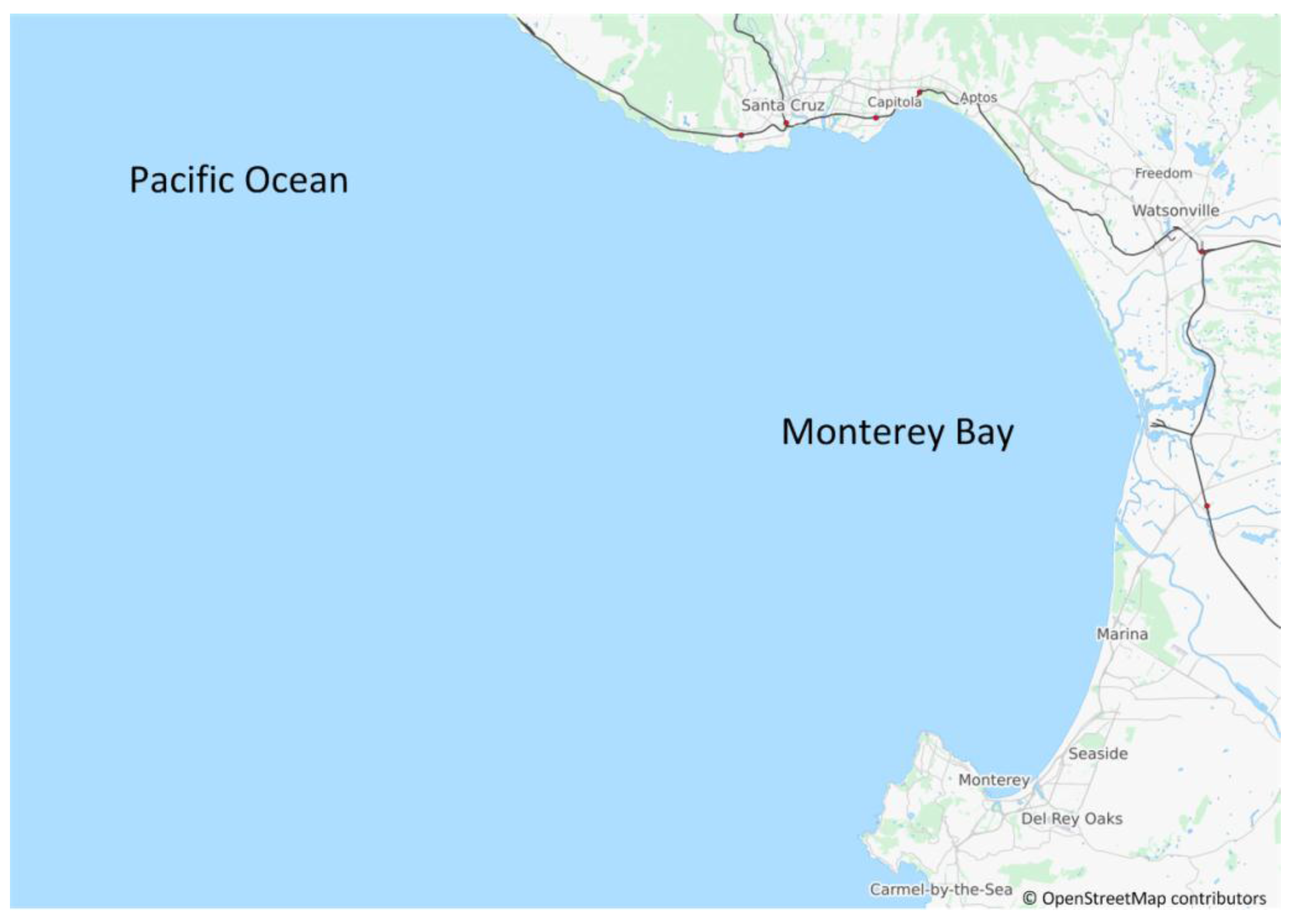
2.1. Study Area

2.2. Satellite Data
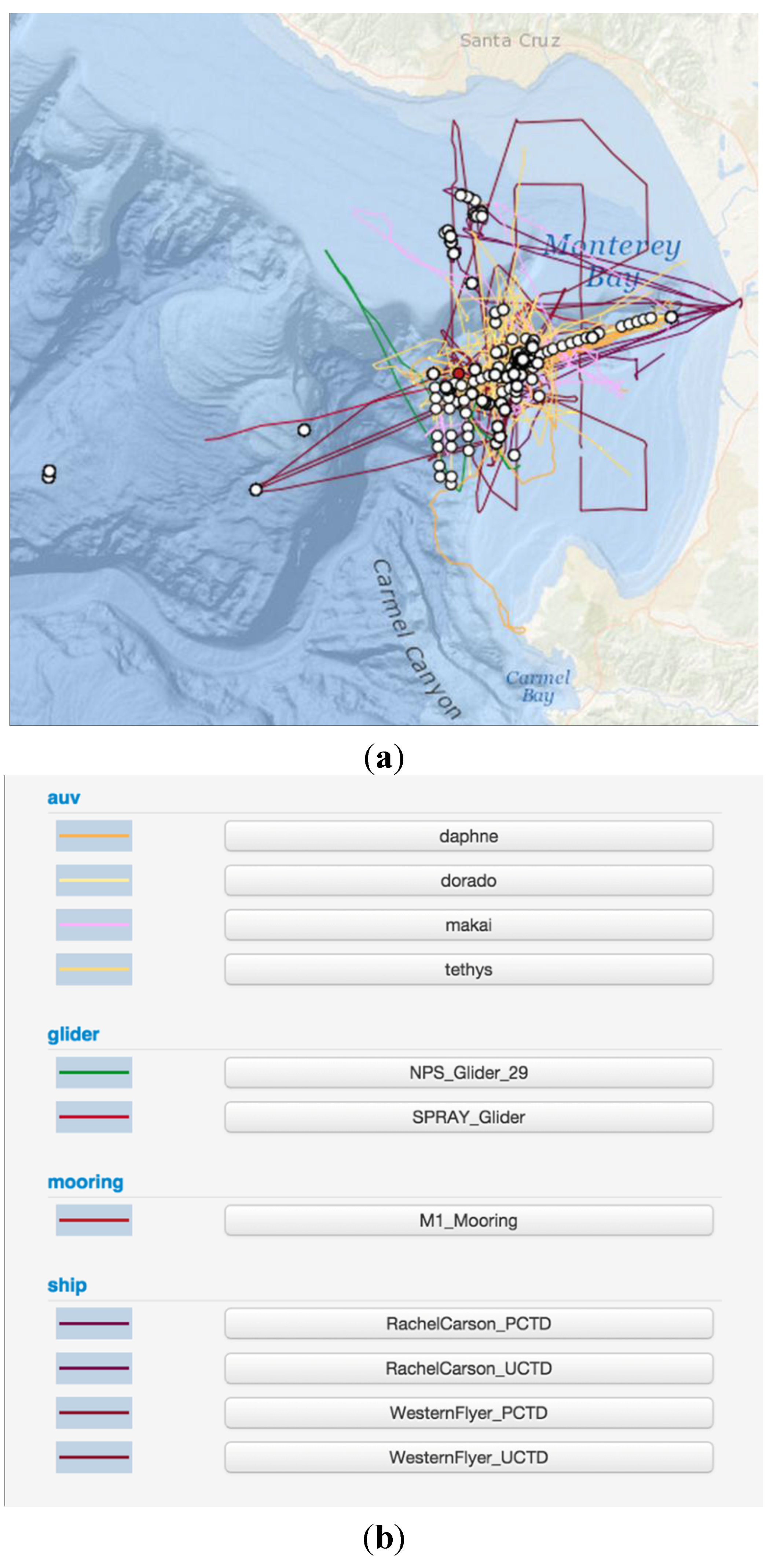
2.3. In Situ Data
3. Satellite Data Analysis
3.1. Feature Extraction for Obtaining Training Input Data
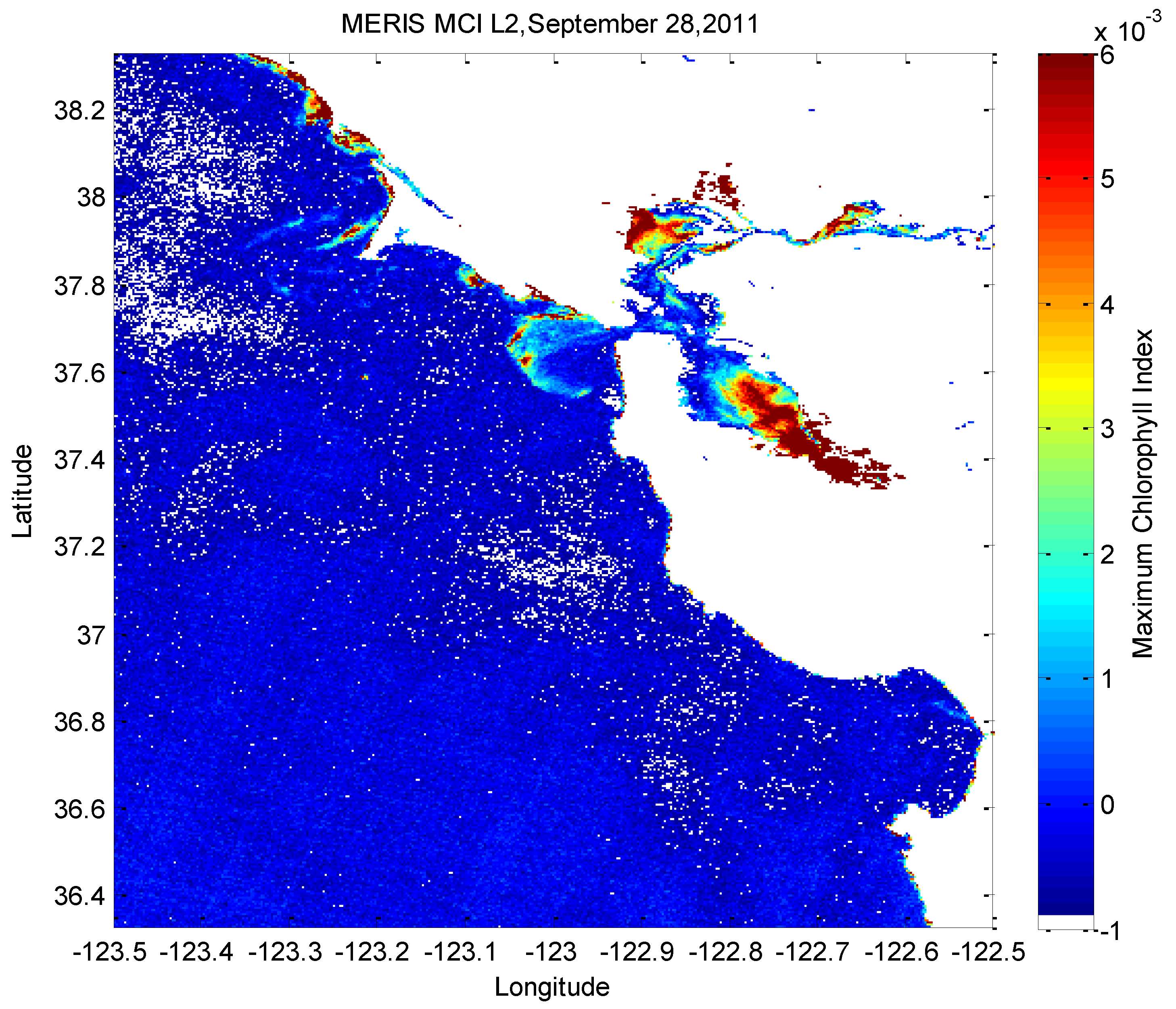
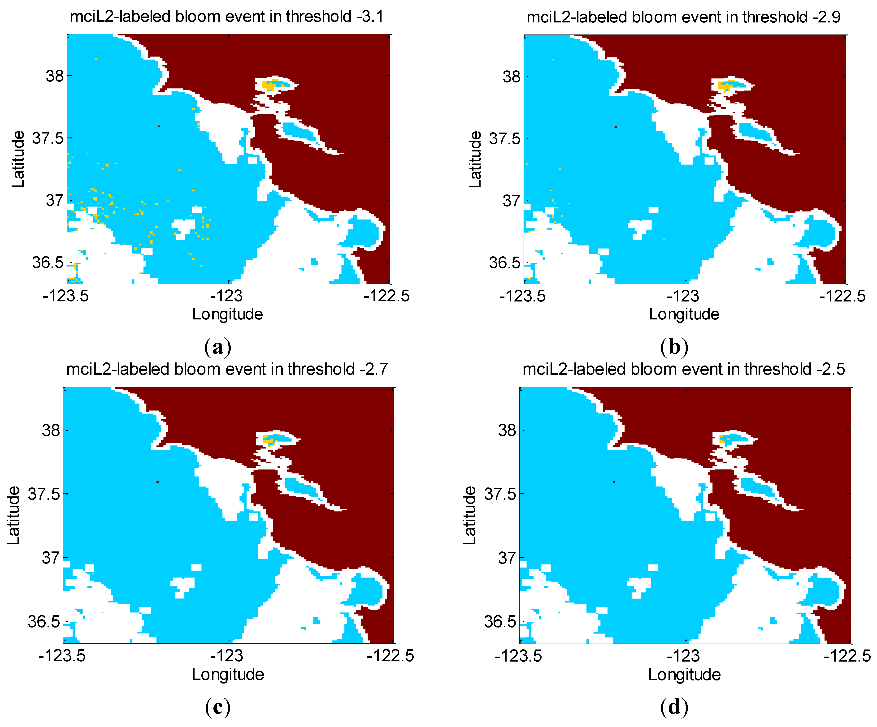
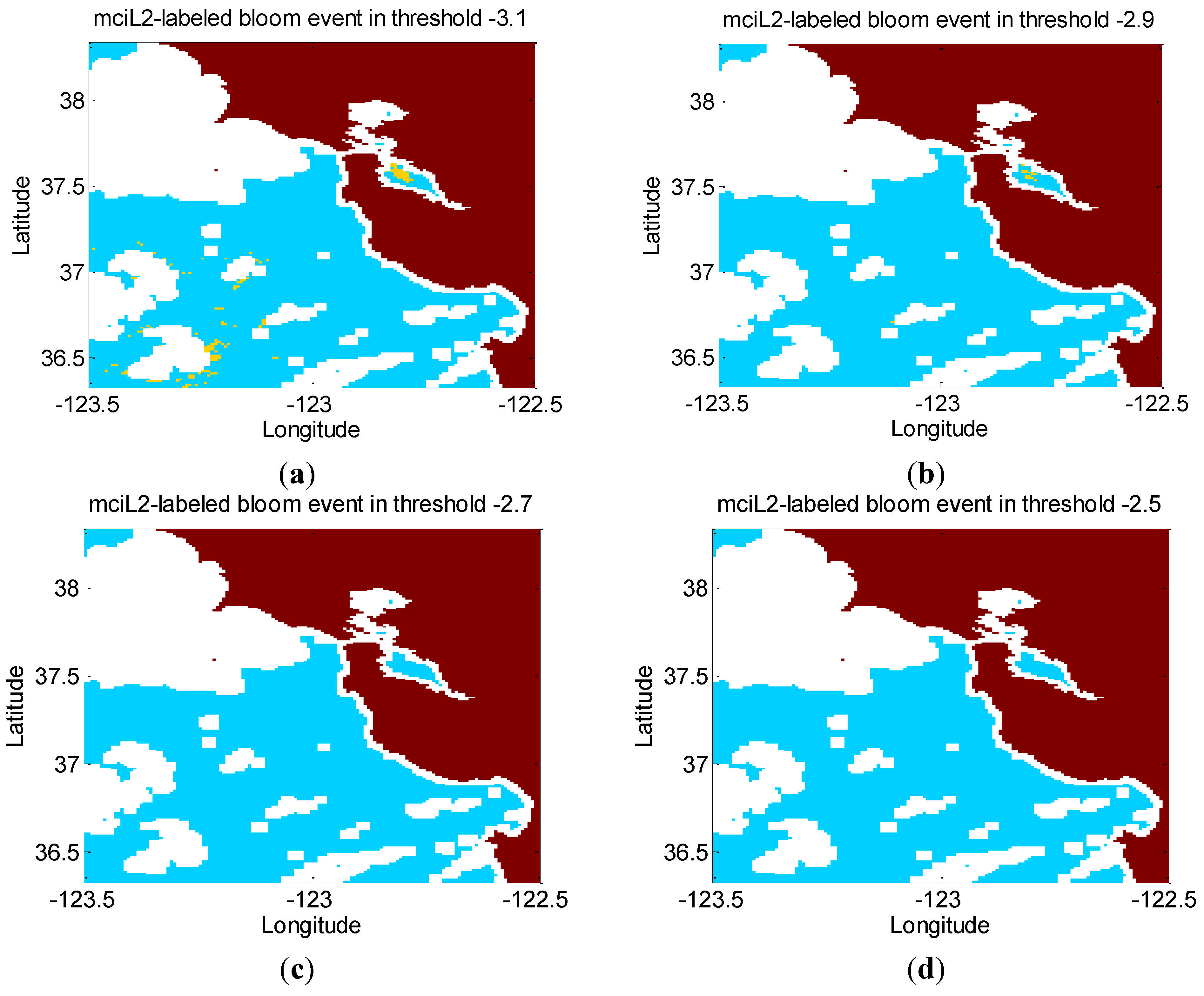
3.2. Threshold Filter for Labeling the MERIS and in Situ Data


4. Machine Learning for Bloom Event Prediction
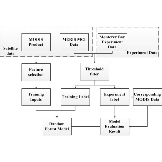
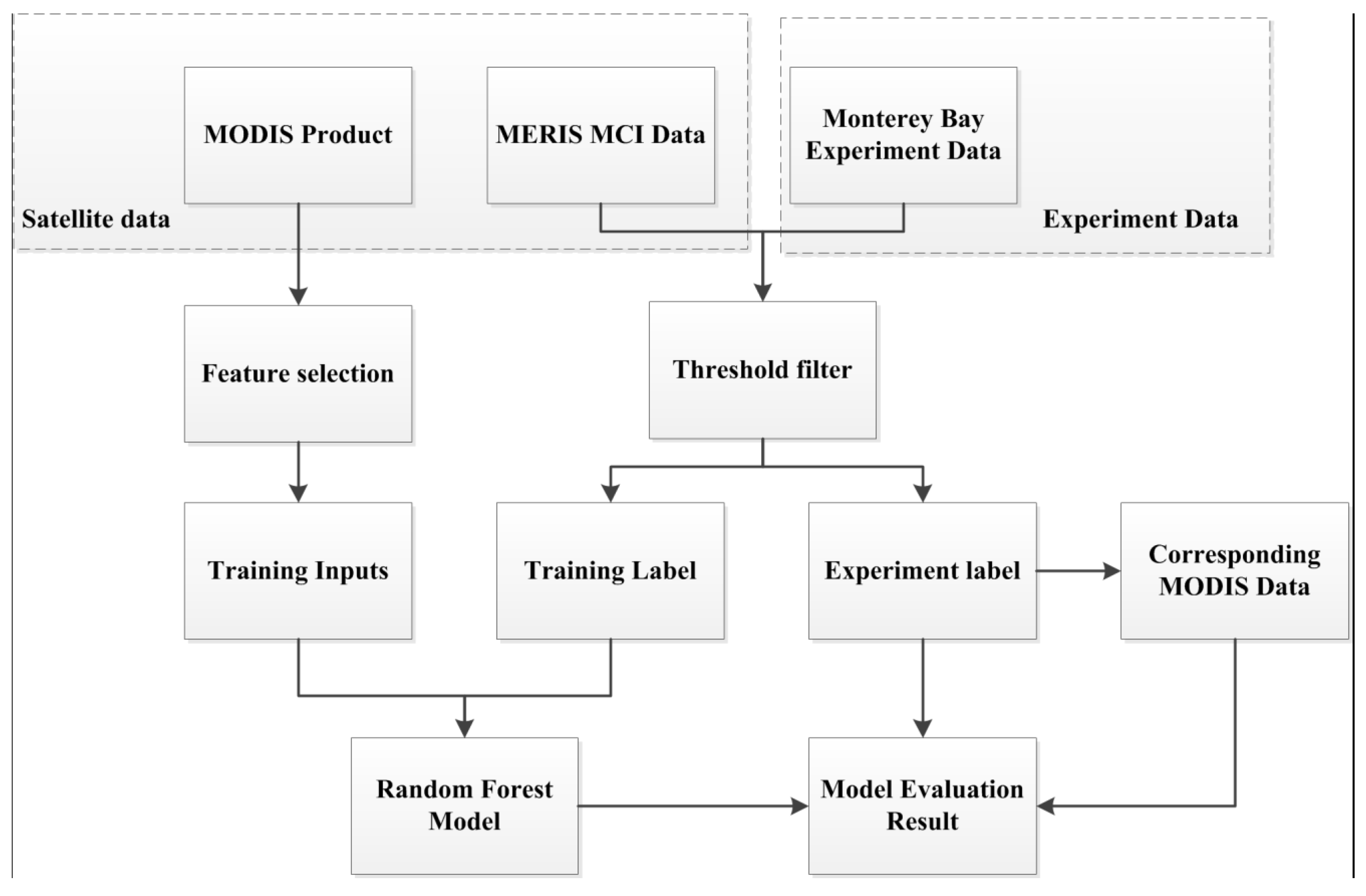
4.1. Overview of the Bloom Event Prediction Framework
4.2. Machine Learning for Classification
4.2.1. Support Vector Machine
4.2.2. Random Forest
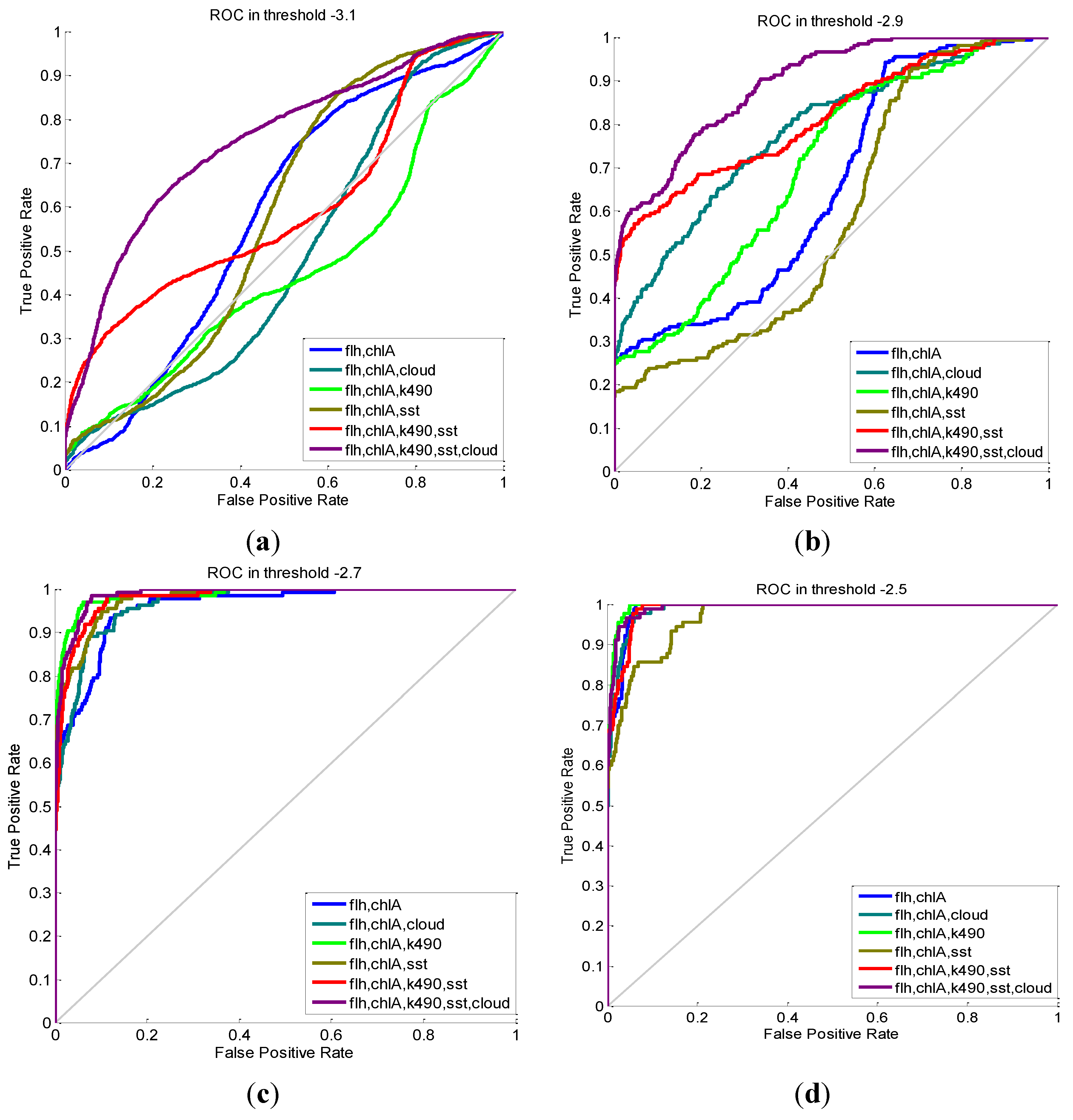
4.2.3. Evaluation Methods
5. Experimental Results
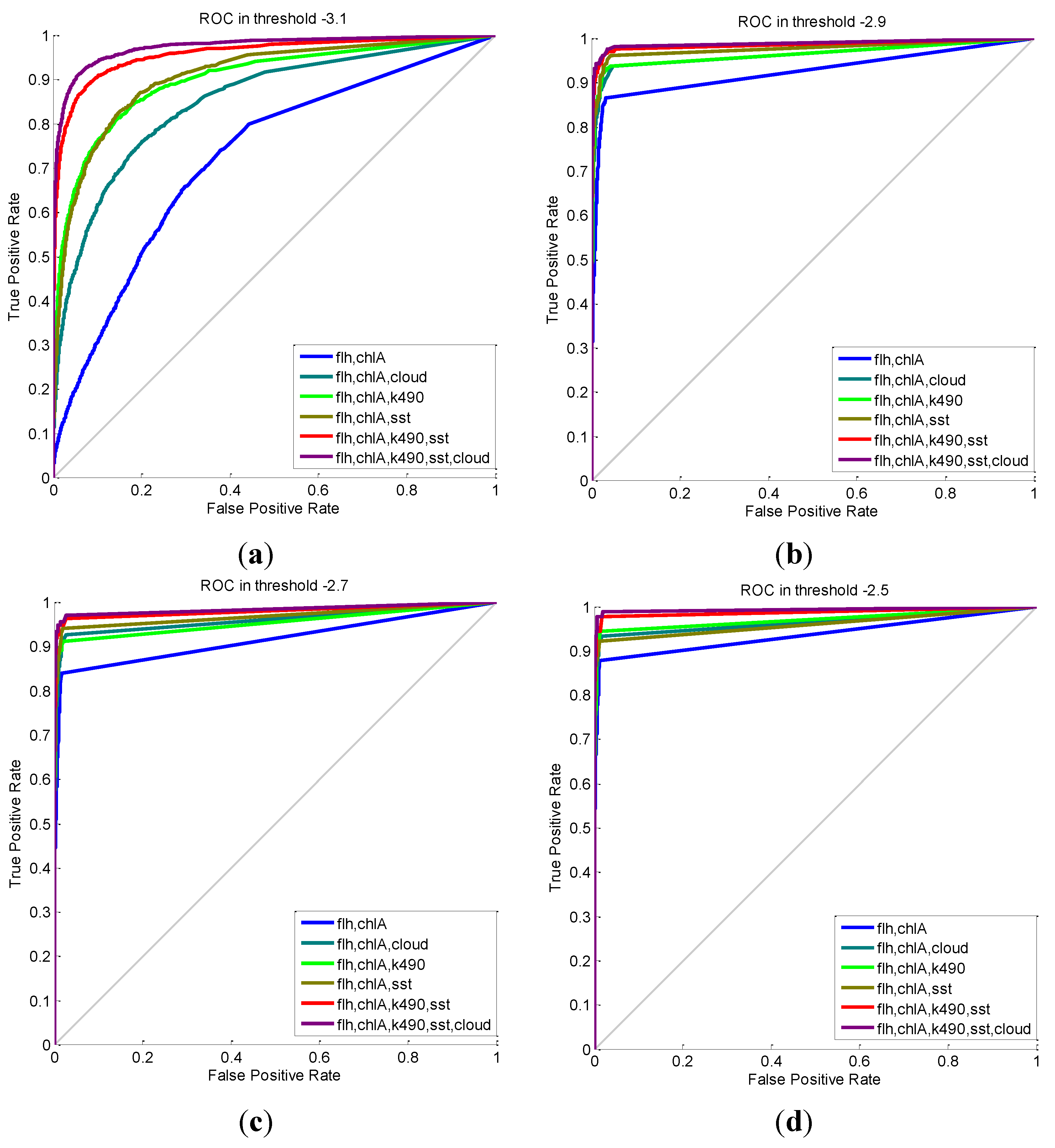
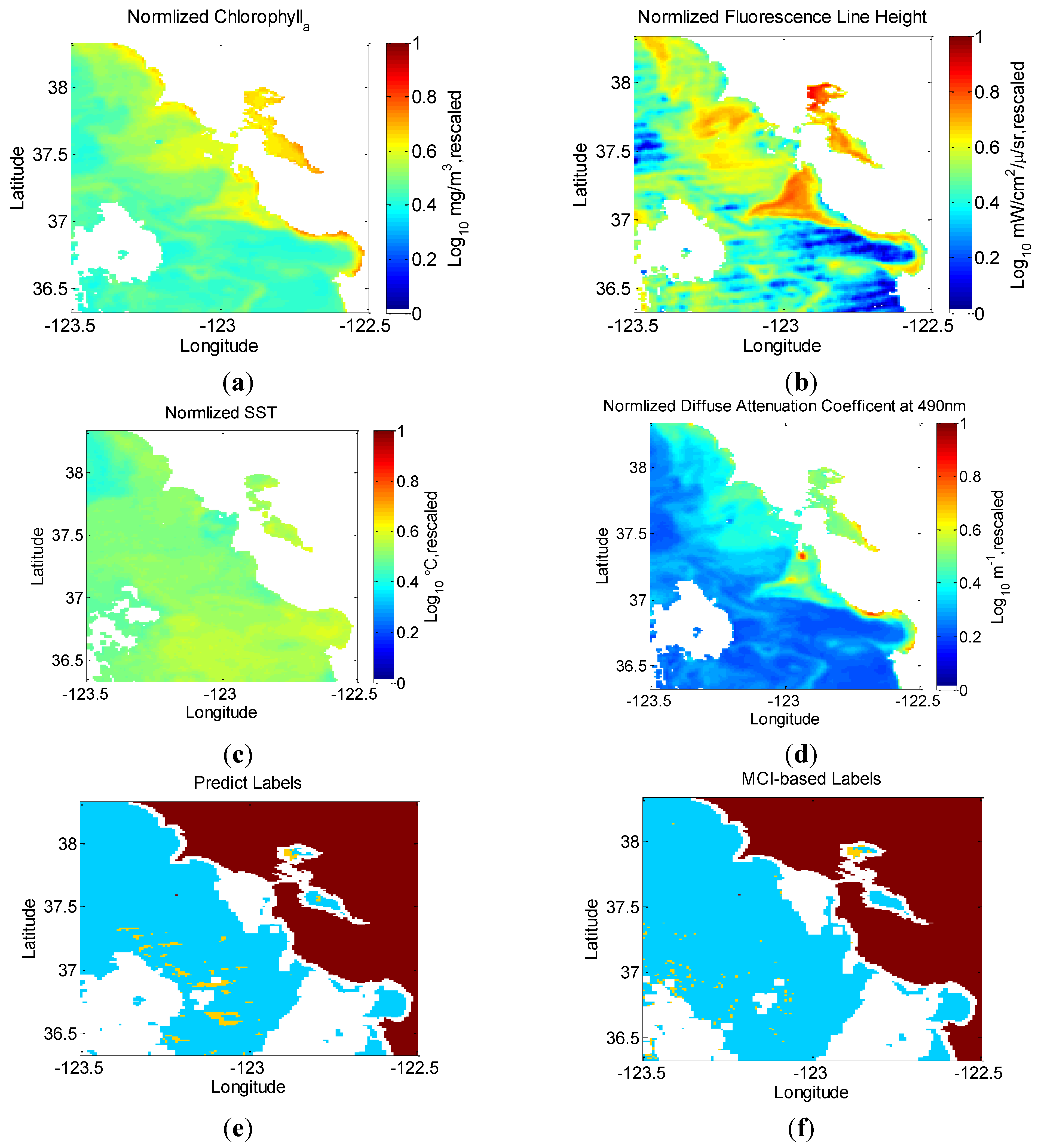
5.1. Evaluation of the MCI-Based Model

| Features | MCC | Accuracy | Recall | Precision | Confusion Matrix (TP, TN, FP, FN) |
|---|---|---|---|---|---|
| flh, chlA | 0.3194 | 0.998 | 0.121 | 0.846 | (11, 47,212, 2, 80) |
| flh, chlA, cloud | 0.3140 | 0.998 | 0.132 | 0.750 | (12, 47,210, 4, 79) |
| flh, chlA, k490 | 0.3403 | 0.998 | 0.143 | 0.813 | (13, 47,211, 3, 78) |
| flh, chlA, sst | 0.3571 | 0.998 | 0.176 | 0.727 | (16, 47,208, 6, 75) |
| flh, chlA, k490, sst | 0.3827 | 0.998 | 0.209 | 0.703 | (19, 47,206, 8, 72) |
| flh, chlA, k490, sst, cloud | 0.5590 | 0.998 | 0.385 | 0.814 | (35, 47,206, 8, 56) |
| Features | MCC | Accuracy | Recall | Precision | Confusion Matrix (TP, TN, FP, FN) |
|---|---|---|---|---|---|
| flh, chlA | 0.4380 | 0.998 | 0.319 | 0.604 | (29, 47,195, 19, 62) |
| flh, chlA, cloud | 0.5637 | 0.999 | 0.451 | 0.707 | (41, 47,197, 17, 50) |
| flh, chlA, k490 | 0.4396 | 0.998 | 0.330 | 0.588 | (30, 47,193, 21, 61) |
| flh, chlA, sst | 0.5775 | 0.999 | 0.462 | 0.724 | (42, 47,198, 16, 49) |
| flh, chlA, k490, sst | 0.6761 | 0.999 | 0.593 | 0.771 | (54, 47,198, 16, 37) |
| flh, chlA, k490, sst, cloud | 0.7062 | 0.999 | 0.615 | 0.812 | (56, 47,201, 13, 35) |
| Features | MCC | Accuracy | Recall | Precision | Confusion Matrix (TP, TN, FP, FN) |
|---|---|---|---|---|---|
| flh, chlA | 0.1168 | 0.962 | 0.535 | 0.311 | (90, 45,425, 199, 1591) |
| flh, chlA, cloud | 0.2864 | 0.965 | 0.164 | 0.545 | (276, 45,394, 230, 1405) |
| flh, chlA, k490 | 0.4633 | 0.971 | 0.329 | 0.688 | (553, 45,373, 251, 1128) |
| flh, chlA, sst | 0.3966 | 0.968 | 0.276 | 0.610 | (464, 45,327, 297, 1217) |
| flh, chlA, k490, sst | 0.6743 | 0.980 | 0.553 | 0.845 | (929, 45,453, 171, 752) |
| flh, chlA, k490, sst, cloud | 0.7321 | 0.983 | 0.622 | 0.880 | (1045, 45,482, 142, 636) |
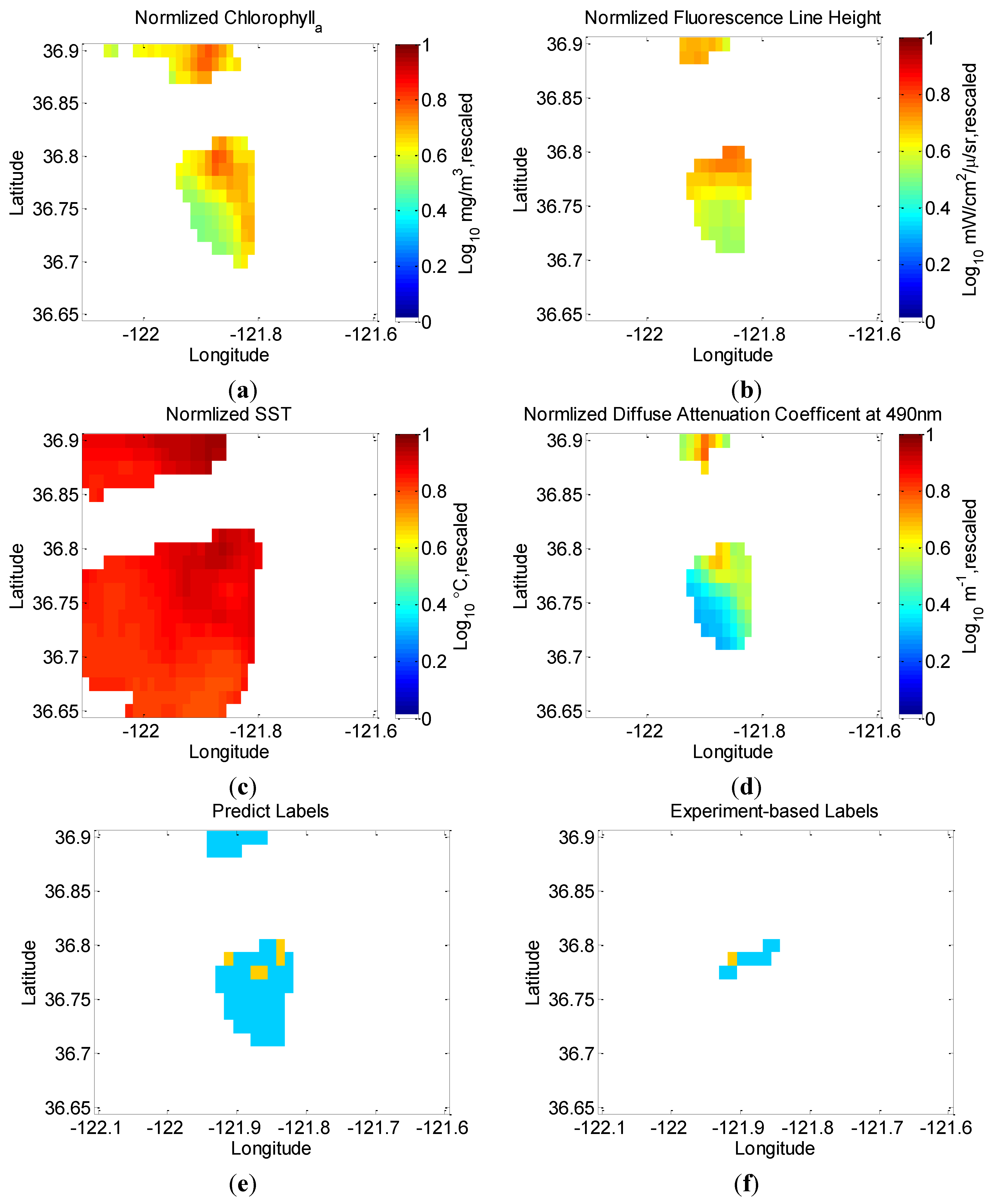
5.2. Evaluation of the Final Model Using in Situ Data from Field Experiment
| Position | Feature Input | Predicted-Label | Maximum Chlorophyll | Experiment-Based Label |
|---|---|---|---|---|
| 36.775°N121.925°W | chlA, flh, k490, sst | 0 | 7.50 | 0 |
| 36.775°N121.9125°W | chlA, flh, k490, sst | 0 | 8.72 | 0 |
| 36.7875°N121.9125°W | chlA, flh, k490, sst | 1 | 14.90 | 1 |
| 36.7875°N121.9°W | chlA, flh, k490, sst | 0 | 6.16 | 0 |
| 36.7875°N121.8875°W | chlA, flh, k490, sst | 0 | 4.14 | 0 |
| 36.7875°N121.875°W | chlA, flh, k490, sst | 0 | 5.51 | 0 |
| 36.7875°N121.8625°W | chlA, flh, k490, sst | 0 | 3.60 | 0 |
| 36.8°N121.8625°W | chlA, flh, k490, sst | 0 | 3.97 | 0 |
| 36.8°N131.85°W | chlA, flh, k490, sst | 0 | 5.77 | 0 |
6. Conclusions
Acknowledgments
Author Contributions
Conflicts of Interest
References
- Bauman, A.G.; Burt, J.A.; Feary, D.A.; Marquis, E.; Usseglio, P. Tropical harmful algal blooms: An emerging threat to coral reef communities? Mar. Pollut. Bull. 2010, 60, 2117–2122. [Google Scholar] [CrossRef] [PubMed]
- Trainer, V.; Pitcher, G.; Reguera, B.; Smayda, T. The distribution and impacts of harmful algal bloom species in eastern boundary upwelling systems. Prog. Oceanogr. 2010, 85, 33–52. [Google Scholar] [CrossRef]
- Li, H.M.; Tang, H.J.; Shi, X.Y.; Zhang, C.S.; Wang, X.L. Increased nutrient loads from the Changjiang (Yangtze) River have led to increased Harmful Algal Blooms. Harmful Algae 2014, 39, 92–101. [Google Scholar] [CrossRef]
- Hoagland, P.; Anderson, D.; Kaoru, Y.; White, A. The economic effects of harmful algal blooms in the United States: Estimates, assessment issues, and information needs. Estuaries 2002, 25, 819–837. [Google Scholar] [CrossRef]
- Hudnell, H.K. The state of US freshwater harmful algal blooms assessments, policy and legislation. Toxicon 2010, 55, 1024–1034. [Google Scholar] [CrossRef] [PubMed]
- Ryan, J.; Dierssen, H.; Kudela, R.; Scholin, C.; Johnson, K.; Sullivan, J.; Fischer, A.; Rienecker, E.; McEnaney, P.; Chavez, F. Coastal ocean physics and red tides: An example from Monterey Bay, California. Oceanography 2005, 18, 246–255. [Google Scholar] [CrossRef]
- Ryan, J.; Fischer, A.; Kudela, R.; McManus, M.; Myers, J.; Paduan, J.; Ruhsam, C.; Woodson, C.; Zhang, Y. Recurrent frontal slicks of a coastal ocean upwelling shadow. J. Geophys. Res. 2010, 115. [Google Scholar] [CrossRef]
- Ryan, J.P.; Gower, J.F.; King, S.A.; Bissett, W.P.; Fischer, A.M.; Kudela, R.M.; Kolber, Z.; Mazzillo, F.; Rienecker, E.V.; Chavez, F.P. A coastal ocean extreme bloom incubator. Geophys. Res. Lett. 2008, 35. [Google Scholar] [CrossRef]
- Allen, J.I.; Smyth, T.J.; Siddorn, J.R.; Holt, M. How well can we forecast high biomass algal bloom events in a eutrophic coastal sea? Harmful Algae 2008, 8, 70–76. [Google Scholar] [CrossRef]
- Gower, J.; King, S.; Borstad, G.; Brown, L. Detection of intense plankton blooms using the 709 nm band of the MERIS imaging spectrometer. Int. J. Remote Sens. 2005, 26, 2005–2012. [Google Scholar] [CrossRef]
- Shen, L.; Xu, H.; Guo, X. Satellite remote sensing of harmful algal blooms (HABs) and a potential synthesized framework. Sensors 2012, 12, 7778–7803. [Google Scholar] [CrossRef] [PubMed]
- Miller, P.I.; Shutler, J.D.; Moore, G.F.; Groom, S.B. SeaWiFS discrimination of harmful algal bloom evolution. Int. J. Remote Sens. 2006, 27, 2287–2301. [Google Scholar] [CrossRef]
- Tomlinson, M.C.; Stumpf, R.P.; Ransibrahmanakul, V.; Truby, E.W.; Kirkpatrick, G.J.; Pederson, B.A.; Vargo, G.A.; Heil, C.A. Evaluation of the use of SeaWiFS imagery for detecting Karenia brevis harmful algal blooms in the eastern Gulf of Mexico. Remote Sens. Environ. 2004, 91, 293–303. [Google Scholar] [CrossRef]
- Matarrese, R.; Morea, A.; Tijani, K.; de Pasquale, V.; Chiaradia, M.T.; Pasquariello, G. A specialized support vector machine for coastal water Chlorophyll retrieval from water leaving reflectances. In Proceedings of the IEEE International Geoscience and Remote Sensing Symposium, Boston, MA, USA, 7–11 July 2008; pp. 910–913.
- Bernstein, M.; Graham, R.; Cline, D.; Dolan, J.M.; Rajan, K. Learning-based event response for marine robotics. In Proceedings of the IEEE International Conference on Intelligent Robots and Systems (IROS), Tokyo, Japan, 3–7 November 2013; pp. 3362–3367.
- Oceanographic Decision Support System. Available online: https://odss.mbari.org/odss/ (accessed on 23 September 2015).
- Gomes, K.; Cline, D.; Edgington, D.; Godin, M.; Maughan, T.; McCann, M.T.; O’Reilly, T.; Bahr, F.; Chavez, F.; Messié, M. Odss: A decision support system for ocean exploration. In Proceedings of the IEEE 29th International Conference on Data Engineering Workshops (ICDEW), Brisbane, Australia, 8–12 April 2013; pp. 200–211.
- Das, J.; Rajan, K.; Frolov, S.; Pyy, F.; Ryan, J.; Caron, D.; Sukhatme, G.S. Towards marine bloom trajectory prediction for AUV mission planning. In Proceedings of the IEEE International Conference on Robotics and Automation (ICRA), Anchorage, AK, USA, 3–7 May 2010; pp. 4784–4790.
- Das, J.; Maughan, T.; McCann, M.; Godin, M.; Reilly, T.O.; Messié, M.; Bahr, F.; Gomes, K.; Py, F.; Bellingham, J.G. Towards mixed-initiative, multi-robot field experiments: Design, deployment, and lessons learned. In Proceedings of the IEEE International Conference on Intelligent Robots and Systems (IROS), San Francisco, CA, USA, 25–30 September 2011; pp. 3132–3139.
- Das, J.; Harvey, J.; Py, F.; Vathsangam, H.; Graham, R.; Rajan, K.; Sukhatme, G. Hierarchical probabilistic regression for AUV-based adaptive sampling of marine phenomena. In Proceedings of the IEEE International Conference on Robotics and Automation (ICRA), Karlsruhe, Germany, 6–10 May 2013; pp. 5571–5578.
- Ryan, J.P.; Davis, C.O.; Tufillaro, N.B.; Kudela, R.M.; Gao, B.C. Application of the hyperspectral imager for the coastal ocean to phytoplankton ecology studies in Monterey Bay, CA, USA. Remote Sens. 2014, 6, 1007–1025. [Google Scholar] [CrossRef]
- Ryan, J.; Greenfield, D.; Marin, R., III; Preston, C.; Roman, B.; Jensen, S.; Pargett, D.; Birch, J.; Mikulski, C.; Doucette, G. Harmful phytoplankton ecology studies using an autonomous molecular analytical and ocean observing network. Limnol. Oceanogr. 2011, 56, 1255–1272. [Google Scholar] [CrossRef]
- Jessup, D.A.; Miller, M.A.; Ryan, J.P.; Nevins, H.M.; Kerkering, H.A.; Mekebri, A.; Crane, D.B.; Johnson, T.A.; Kudela, R.M. Mass stranding of marine birds caused by a surfactant-producing red tide. PLoS ONE 2009, 4, e4550. [Google Scholar] [CrossRef]
- Kudela, R.M.; Lane, J.Q.; Cochlan, W.P. The potential role of anthropogenically derived nitrogen in the growth of harmful algae in California, USA. Harmful Algae 2008, 8, 103–110. [Google Scholar] [CrossRef]
- Binding, C.; Greenberg, T.; Bukata, R. The MERIS maximum chlorophyll index; its merits and limitations for inland water algal bloom monitoring. J. Great Lakes Res. 2013, 39, 100–107. [Google Scholar] [CrossRef]
- Hu, C.; Cannizzaro, J.; Carder, K.L.; Muller-Karger, F.E.; Hardy, R. Remote detection of Trichodesmium blooms in optically complex coastal waters: Examples with MODIS full-spectral data. Remote Sens. Environ. 2010, 114, 2048–2058. [Google Scholar] [CrossRef]
- Justice, C.O.; Vermote, E.; Townshend, J.R.G.; DeFries, R.; Roy, D.P.; Hall, D.K.; Salomonson, V.V.; Privette, J.L.; Riggs, G.; Strahler, A.; et al. The Moderate Resolution Imaging Spectroradiometer (MODIS): Land remote sensing for global change research. IEEE Trans. Geosci. Remote Sens. 1998, 36, 1228–1249. [Google Scholar] [CrossRef]
- Rast, M.; Bezy, J.; Bruzzi, S. The ESA Medium Resolution Imaging Spectrometer MERIS a review of the instrument and its mission. Int. J. Remote Sens. 1999, 20, 1681–1702. [Google Scholar] [CrossRef]
- Campaign List. Available online: http://odss.mbari.org/canon (accessed on 23 September 2015).
- Stoqs_September 2014. Available online: http://odss.mbari.org/canon/stoqs_september2014/query/ (accessed on 23 September 2015).
- Stramska, M.; Świrgoń, M. Influence of atmospheric forcing and freshwater discharge on interannual variability of the vertical diffuse attenuation coefficient at 490 nm in the Baltic Sea. Remote Sens. Environ. 2014, 140, 155–164. [Google Scholar] [CrossRef]
- Wang, S.; Tang, D. Remote sensing of day/night sea surface temperature difference related to phytoplankton blooms. Int. J. Remote Sens. 2010, 31, 4569–4578. [Google Scholar] [CrossRef]
- Bishop, C. Pattern Recognition and Machine Learning (Information Science and Statistics), 2nd ed.; Springer: New York, NY, USA, 2007. [Google Scholar]
- Baldi, P.; Brunak, S.; Chauvin, Y.; Andersen, C.A.; Nielsen, H. Assessing the accuracy of prediction algorithms for classification: An overview. Bioinformatics 2000, 16, 412–424. [Google Scholar] [CrossRef] [PubMed]
- Chang, C.C.; Lin, C.J. LIBSVM: A library for support vector machines. ACM Trans. Intell. Syst. Technol. 2011, 2, 27. [Google Scholar] [CrossRef]
- Breiman, L. Random forests. Mach. Learn. 2001, 45, 5–32. [Google Scholar] [CrossRef]
- Breiman, L. Bagging predictors. Mach. Learn. 1996, 24, 123–140. [Google Scholar] [CrossRef]
- Stehman, S.V. Selecting and interpreting measures of thematic classification accuracy. Remote Sens. Environ. 1997, 62, 77–89. [Google Scholar] [CrossRef]
- Fawcett, T. An introduction to ROC analysis. Pattern Recognit. Lett. 2006, 27, 861–874. [Google Scholar] [CrossRef]
© 2015 by the authors; licensee MDPI, Basel, Switzerland. This article is an open access article distributed under the terms and conditions of the Creative Commons Attribution license (http://creativecommons.org/licenses/by/4.0/).
Share and Cite
Song, W.; Dolan, J.M.; Cline, D.; Xiong, G. Learning-Based Algal Bloom Event Recognition for Oceanographic Decision Support System Using Remote Sensing Data. Remote Sens. 2015, 7, 13564-13585. https://doi.org/10.3390/rs71013564
Song W, Dolan JM, Cline D, Xiong G. Learning-Based Algal Bloom Event Recognition for Oceanographic Decision Support System Using Remote Sensing Data. Remote Sensing. 2015; 7(10):13564-13585. https://doi.org/10.3390/rs71013564
Chicago/Turabian StyleSong, Weilong, John M. Dolan, Danelle Cline, and Guangming Xiong. 2015. "Learning-Based Algal Bloom Event Recognition for Oceanographic Decision Support System Using Remote Sensing Data" Remote Sensing 7, no. 10: 13564-13585. https://doi.org/10.3390/rs71013564
APA StyleSong, W., Dolan, J. M., Cline, D., & Xiong, G. (2015). Learning-Based Algal Bloom Event Recognition for Oceanographic Decision Support System Using Remote Sensing Data. Remote Sensing, 7(10), 13564-13585. https://doi.org/10.3390/rs71013564