Ocean Wave Parameters Retrieval from TerraSAR-X Images Validated against Buoy Measurements and Model Results

Abstract

An ocean surface wave retrieval algorithm, Parameterized First-guess Spectrum Method (PFSM), which was initially developed for C-band Synthetic Aperture Radar (SAR), is modified to extract wave parameters from X-band TerraSAR-X (TS-X) images. Wave parameters, including significant wave height (SWH) and mean wave period (MWP) were extracted from nine TS-X HH-polarization images and were compared to in situ buoy measurements. The range of these wave retrievals is from 1 to 5 m of SWH and from 2 to 10 s of MWP. The retrieval accuracy could reach 80%. After that, a total of 16 collected TS-X HH-polarization images were used to invert wave parameters and then the retrieval results were compared to the operational WAVEWATCH-III wave model results. The SAR and in situ buoy wave comparison shows a 0.26 m Root-Mean-Square Error (RMSE) of SWH and a 19.8% of Scatter Index (SI). The SAR and WAVEWATCH-III model comparison yields slightly worse results with an RMSE of 0.43 m of SWH and a 32.8% of SI. For MWP, the SAR and buoy comparison shows the RMSE is 0.45 s with an SI of 26%, which is better than the results from the SAR and WAVEWATCH-III model comparison. Our results show that the PFSM algorithm is suitable to estimate wave parameters from X-band TS-X data.

1. Introduction

With high spatial resolution, relatively large swath and all-weather imaging capability, Synthetic Aperture Radar (SAR) is an efficient instrument providing data to derive sea surface wind and wave parameters. SAR sensors usually operate in C-band (ERS-1/2, EnviSAT-ASAR, and RadarSAT-1/2), L-band (SEASAT, ALOS-11/2), and X-band (such as TerraSAR-X (TS-X), TanDEM-X (TD-X), and Cosmo-SkyMed). To date, wind and wave retrieval algorithms have usually been based on empirical Geophysical Model Function (GMF) algorithms. These algorithms are more mature for C-band SAR but less for the newer X-band SARs. The TS-X and TD-X were launched in 2007 and 2010, respectively. Their orbital height and period are 514 kilometers and 100 minutes. Both satellites carry an X-band (9.8 GHz) SAR sensor with high spatial resolution up to 1 m. Much effort has been made to derive applications for oceanography. For sea surface wind field retrievals, similar to C-band wind field measurements, several X-band GMFs were developed from SAR in vertical-vertical (VV) [1,2] and horizontal-horizontal (HH) polarization based on the Polarization Ratio (PR) model [3]. For wave measurements, the SAR imaging of sea surface wave is a topic of active research. In general, the SAR backscatter signal is dominated by ocean surface Bragg waves [4]. According to the two-scale model [5], tilt modulation and hydrodynamic modulation on short waves are considered to be the dominating factors for imaging ocean waves. There is a unique modulation of ocean wave on SAR due to the orbital motion of the waves, which is referred to as velocity bunching. This modulation is a non-linear mechanism, which is caused by distortions induced by ocean wave motions, which propagate in the radar azimuthal (parallel to the satellite flight) direction. The result of velocity bunching is that SAR cannot detect specific waves in the azimuth direction [6,7], due to the loss of information beyond a cut-off wave number with an ocean wavelength shorter than 200 m.

The basic scattering physics that is commonly used in wave retrieval algorithms, i.e., Max-Planck Institute Algorithm (MPI), Semi Parametric Retrieval Algorithm Scheme (SPRA) and Parameterized First-guess Spectrum Method (PFSM), are not radar frequency dependent. This study is an application of one such algorithm for wave retrieval using X-band SAR data. Historically, the first wave algorithm named the MPI [8,9,10] was based on C-band ERS SAR data. Later on, the SPRA [11] was developed on the basis of the same modulation mechanism. These algorithms use empirical functions, such as JONSWAP [12] to invert the wind–sea wave spectrum, and satellite scatterometer to get wind data. The SPRA algorithm then does a forward simulation until the simulated SAR spectrum is closest to the actual SAR image spectrum. The difference between the simulated SAR spectra of the best-inverted wind–sea wave spectrum and the observed SAR intensity spectrum is supposed to be determined by the swell. The SPRA scheme is easier to implement than the MPI. A validation study using in situ buoy data showed that the SPRA is better than the MPI [13]. Theoretically, the error of the SPRA scheme is embedded in the swell SAR spectrum retrieval. To overcome the model-induced swell spectrum error, the PFSM was developed [14,15]. Firstly, the SAR intensity spectrum is divided into two parts: the SAR portion of wind–sea and the linear-mapping swell. As for the wind–sea portion, the best first-guess spectrum is obtained by searching for the most suitable parameters in an empirical wave model such as JONSWAP, Pierson–Moscowitz (PM), etc., and then the MPI scheme is employed for the wave spectrum retrieval. The linear-mapping swell spectrum is acquired by directly inverting the given portion of the SAR spectrum generated by swell. Thus, PFSM, which is based on a SAR imaging mechanism [4] like MPI, allows for the quick estimation of wave parameters similar to SPRA.

For C-band SAR, there are several empirical algorithms for wave parameter retrieval, i.e., CWAVE_ERS [16] and CWAVE_ENVI [17,18]. Since TS-X achieves high quality SAR images with fine resolution up to 1m, it is essential to develop a method that can detect wave information from a TS-X image. An empirical algorithm called XWAVE has been proposed [17,19], which is tuned from a few datasets including the two-dimensional intensity spectrum from TS-X, wave parameters from the global atmospheric-marine model provided by the German Weather Service (DWD), buoys, etc. XWAVE is an attempt at wave retrieval, which generates quick results from TS-X, as the function of XWAVE is defined as a linear relationship between sea state and other variables such as wind, SAR intensity spectrum, etc.

Although existing TS-X wave retrievals are focused on an empirical approach, the empirical model XWAVE is not improved in this paper. Nevertheless the PFSM is first validated for X-band SAR. An appropriate modification in the scheme of PFSM is that wind vector, which is derived from TS-X with the same spatial resolution as the waves, is used to produce wind–sea spectra to enhance the accuracy of inversion. In Section 2, data used in our study is introduced. The methodology for wind vector retrieval, that is a necessary preliminary, is briefly represented here, and the PFSM scheme for wave retrieval from TS-X is described in Section 3. In Section 4, the retrieval results are compared to in situ buoy measurements and the results from the numeric wave model to confirm the validation of PFSM. Conclusions are given in Section 5.

2. Satellite and Buoy Data

A total of 16 StripMap mode TS-X images were collected in our study, and the detailed information for each image is presented in Table 1. Normalized radar cross section (NRCS) can be obtained from these calibrated SAR images, and used as input to calculate sea surface wind fields [17,20,21,22,23,24]. In this study, the European Centre for Medium-Range Weather Forecasts (ECMWF) wind direction data are used for SAR wind speed calculation. ECMWF wind products have a 0.25° × 0.25° spatial resolution while our TS-X data has a 5 spatial resolution. In this study, we extracted wind direction from a two-dimensional SAR image spectrum for wavelengths between 800 and 3000 m [4] with a 180° ambiguity. Then we applied low-resolution ECMWF wind directions to remove that 180° ambiguity. The original SAR NRCS image overlaid on the wind vectors derived from the HH-polarization TS-X image taken at 3:54 p.m. UTC on 29 October 2011 is shown in Figure 1a. The wind information is needed for wave retrieval. In Figure 1b, the ambient wind field is from ECMWF, in which the black rectangle represents the coverage of TS-X shown in Figure 1a. The black arrow represents the wind direction derived from TS-X, which is at the same location as the buoy. SAR wind direction retrieval is calculated from the image spectrum that inherently has a 180° ambiguity. In order to eliminate this ambiguity, we used ECMWF model wind product that provides general background wind direction. The SAR image provides a lot more detailed wind information than the model output.

Table 1. Technical parameters of the sixteen HH-polarization TS-X images used in this study.

Time (UTC)	Swath (Km)	Incidence Angle (°)	Range×Azimuth Resolution (m)	Center Location(°W, °N)
6 February 2008 02:00	5 × 3	29.6–32.6	1.25 × 1.25	122.5, 37.2
22 February 2008 02:08	5 × 3	41.6–44.0	1.25 × 1.25	123,2, 38.1
3 December 2008 05:39	8 × 10	22.3–32.5	8.25 × 8.25	179.3, 51.3
29 January 2009 23:56	8 × 10	22.3–34.9	8.25 × 8.25	90.3, 25.8
22 July 2009 17:03	5 × 3	34.0–36.7	1.25 × 1.25	160.6, 54.3
12 August 2009 04:14	5 × 3	31.8–34.6	1.25 × 1.25	153.9, 22.9
5 December 2010 22:50	15 × 10	22.3–32.7	8.25 × 8.25	75.1, 35.5
13 December 2010 16:19	15 × 10	22.3–32.5	8.25 × 8.25	154.1, 23.4
24 December 2010 16:19	15 × 10	19.7–30.3	8.25 × 8.25	153.8, 23.5
13 March 2011 14:07	15 × 10	37.9–45.6	8.25 × 8.25	121.1, 35.2
29 October 2011 15:54	5 × 3	31.8–34.6	1.25 × 1.25	142.4, 55.8
5 November 2011 02:30	5 × 3	24.9–28.1	1.25 × 1.25	122.4, 37.2
23 January 2012 22:20	5 × 3	31.7–34.6	1.25 × 1.25	64.9, 21.1
25 January 2012 21:51	5 × 3	22.3–25.6	1.25 × 1.25	62.1, 42.2
29 January 2012 10:03	5 × 3	34.0–36.7	1.25 × 1.25	58.0, 43.0
5 February 2012 02:56	5 × 3	36.0–38.6	1.25 × 1.25	138.8, 53.9

Table 1. Technical parameters of the sixteen HH-polarization TS-X images used in this study.

Time (UTC)	Swath (Km)	Incidence Angle (°)	Range×Azimuth Resolution (m)	Center Location(°W, °N)
6 February 2008 02:00	5 × 3	29.6–32.6	1.25 × 1.25	122.5, 37.2
22 February 2008 02:08	5 × 3	41.6–44.0	1.25 × 1.25	123,2, 38.1
3 December 2008 05:39	8 × 10	22.3–32.5	8.25 × 8.25	179.3, 51.3
29 January 2009 23:56	8 × 10	22.3–34.9	8.25 × 8.25	90.3, 25.8
22 July 2009 17:03	5 × 3	34.0–36.7	1.25 × 1.25	160.6, 54.3
12 August 2009 04:14	5 × 3	31.8–34.6	1.25 × 1.25	153.9, 22.9
5 December 2010 22:50	15 × 10	22.3–32.7	8.25 × 8.25	75.1, 35.5
13 December 2010 16:19	15 × 10	22.3–32.5	8.25 × 8.25	154.1, 23.4
24 December 2010 16:19	15 × 10	19.7–30.3	8.25 × 8.25	153.8, 23.5
13 March 2011 14:07	15 × 10	37.9–45.6	8.25 × 8.25	121.1, 35.2
29 October 2011 15:54	5 × 3	31.8–34.6	1.25 × 1.25	142.4, 55.8
5 November 2011 02:30	5 × 3	24.9–28.1	1.25 × 1.25	122.4, 37.2
23 January 2012 22:20	5 × 3	31.7–34.6	1.25 × 1.25	64.9, 21.1
25 January 2012 21:51	5 × 3	22.3–25.6	1.25 × 1.25	62.1, 42.2
29 January 2012 10:03	5 × 3	34.0–36.7	1.25 × 1.25	58.0, 43.0
5 February 2012 02:56	5 × 3	36.0–38.6	1.25 × 1.25	138.8, 53.9

Of the 16 SAR images, nine images cover the buoy locations provided from NOAA (National Oceanic and Atmospheric Administration) National Buoy Center (NDBC). Hourly buoy measurements of wind, significant wave height (SWH) and mean wave period (MWP) closest to these nine SAR imaging times are given in Table 2. We also collected the same wave parameters from the WAVEWATCH-III (c) model (that version is developed at IFREMER) [25], which is the third generation wave model, and the data is openly provided by the IFREMER group.

Table 2. The details of the in situ buoy collected from NDBC. Note that WDIR is wind direction in degree, WSPD is wind speed in meters per second and SWH is significant wave height in meters and MWP is the mean wave period in seconds.

Geographic Coordinate (°W, °N)	Time (UTC)	in situ				SAR-derived
		WDIR	WSPD	SWH	MWP	WDIR	WSPD
122.8, 37.7	6 February 2008	330	7.9	2.28	7.48	317	6.4
123.3, 38.2	22 February 2008	283	5.9	3.39	7.40	274	4.8
89.7, 25.9	29 January 2009	29	10.1	1.46	5.13	33	8.2
75.4, 35.0	5 December 2010	313	11.4	1.90	4.82	303	13.5
153.9, 23.6	13 December 2010	134	6.7	1.85	5.62	137	4.8
153.9, 23.6	24 December 2010	182	5.0	1.76	6.43	206	4.3
120.9, 35.0	13 March 2011	330	4.5	2.13	8.86	350	3.4
142.5, 55.9	20 October 2011	241	12.1	3.26	6.12	240	9.5
64.9, 21.1	23 January 2012	78	8.2	1.76	5.10	63	7.4

Table 2. The details of the in situ buoy collected from NDBC. Note that WDIR is wind direction in degree, WSPD is wind speed in meters per second and SWH is significant wave height in meters and MWP is the mean wave period in seconds.

Geographic Coordinate (°W, °N)	Time (UTC)	in situ				SAR-derived
		WDIR	WSPD	SWH	MWP	WDIR	WSPD
122.8, 37.7	6 February 2008	330	7.9	2.28	7.48	317	6.4
123.3, 38.2	22 February 2008	283	5.9	3.39	7.40	274	4.8
89.7, 25.9	29 January 2009	29	10.1	1.46	5.13	33	8.2
75.4, 35.0	5 December 2010	313	11.4	1.90	4.82	303	13.5
153.9, 23.6	13 December 2010	134	6.7	1.85	5.62	137	4.8
153.9, 23.6	24 December 2010	182	5.0	1.76	6.43	206	4.3
120.9, 35.0	13 March 2011	330	4.5	2.13	8.86	350	3.4
142.5, 55.9	20 October 2011	241	12.1	3.26	6.12	240	9.5
64.9, 21.1	23 January 2012	78	8.2	1.76	5.10	63	7.4

Figure 1. (a) The quick-look example of HH-polarization TS-X image taken at 3:54 p.m. UTC on 29 October 2011 after calibration and wind field retrieval with the corresponding buoy; (b) ECMWF wind field collected at 6:00 p.m., noting that the black rectangle represents the geographic location of TS-X; and (c) the black arrow represents the wind direction derived from TS-X at the buoy location.

Figure 1. (a) The quick-look example of HH-polarization TS-X image taken at 3:54 p.m. UTC on 29 October 2011 after calibration and wind field retrieval with the corresponding buoy; (b) ECMWF wind field collected at 6:00 p.m., noting that the black rectangle represents the geographic location of TS-X; and (c) the black arrow represents the wind direction derived from TS-X at the buoy location.

3. SAR Wave Parameter Retrieval Methodology

As introduced in Section 1, MPI, SPRA or PFSM all require the first “guess” wave spectrum. Firstly, the empirical wave model for producing the “guess” wave spectrum is briefly described below. Following this, the methodology for wind and wave retrieval from SAR is introduced.

3.1. Empirical Wave Model

The two-dimensional “guess” wave spectrum W(k,θ) in terms of wave number $k$ and propagation direction $\text{θ}$ is described as follows:

$$W(k,\text{θ})=W(\text{ω})\times G(\text{θ})\times \frac{d\text{ω}}{dk}$$

(1)

where W(ω) is the one-dimensional JONSWAP spectrum referred to in [12] in terms of frequency ω,

$$W(\text{ω})=\text{α}\frac{g^2}{{\text{ω}}^5}\exp (-1.25{(\frac{{\text{ω}}_0}{\text{ω}})}^4){\text{γ}}^{\exp (-\frac{{(\text{ω}-{\text{ω}}_0)}^2}{2{\text{σ}}^2{\text{ω}}_0^2})}$$

(2)

$\text{α}=0.006{(U_{10}/C_p)}^{0.55}$, γ is the peak-enhancement constant (=3.3), σ is a peak-width parameter and ${\text{ω}}^2=gk$, ${\text{ω}}_0=g/C_p$, in which C_p is peak velocity. The directional function G(θ), which gives the normalized distribution of the wave energy density over direction θ, is described in [15] as sech² style,

$$G(\text{θ})=0.5\cdot \text{β}{\text{sech}}^2\left(\text{β}\left[\text{θ}-{\text{θ}}_m\right]\right)$$

(3)

where, β is the coefficient dependent on various conditions over the wave number $k$ and θ_m is taken as the peak wave direction.

Referring to Equations (1)–(3), the two-dimensional wave spectrum W(k, θ) can be determined only by peak wave phase speed C_p and 180° ambiguity wave direction θ_m, which can be directly obtained from the two-dimensional TS-X intensity spectrum for wavelengths between 25 and 1200 m, and wind speed U₁₀ that is inverted from the TS-X image. The one-dimensional spectrum W(k) is obtained by integrating over all directions,

$$W\text{(}k\text{)}={\displaystyle {\int }_0^{2\pi }W(k,\text{θ})}d\text{θ}$$

(4)

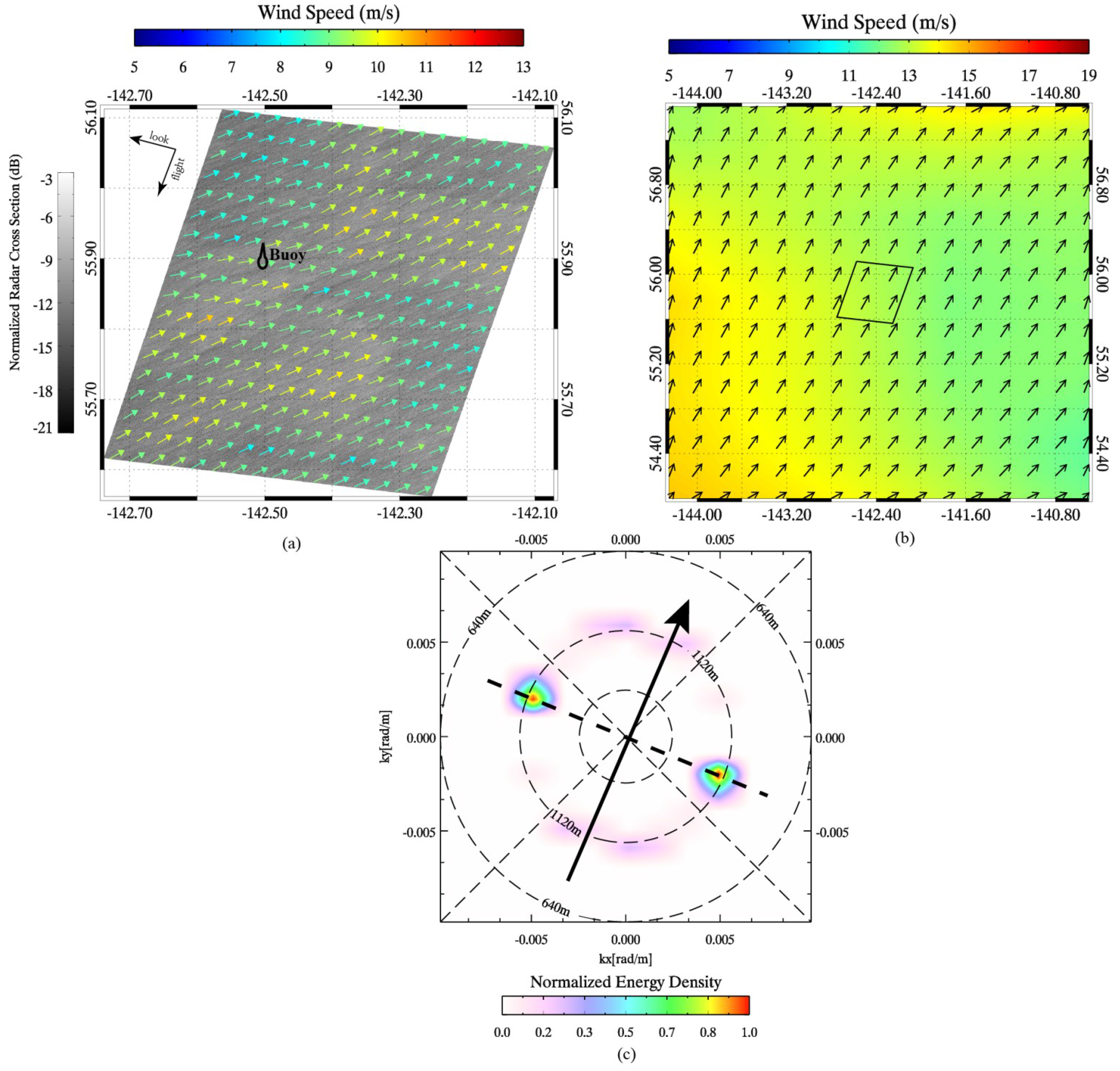
3.2. SAR Wind Retrieval

XMOD2 [1] is developed for wind retrieval from TS-X, acquired in VV-polarization. XMOD2 between the wind vector and NRCS in VV-polarization and takes the form of:

$${\text{σ}}^0=B_0\left(U_{10},\text{θ}\right)\left[1+B_1\left(U_{10},\text{θ}\right)\cos \text{ϕ}+B_2\left(U_{10},\text{θ}\right)\cos 2\text{ϕ}\right]$$

(5)

where σ⁰ is the NRCS in the VV-polarization, φ represents the angle between the radar look direction and the wind direction, θ is the incidence angle, and coefficients B_n are functions of sea surface wind speed and radar incidence angle.

Before XMOD2 is applied, Polarization Ratio (PR) [3] is necessarily used to convert HH-polarization NRCS ${\text{σ}}_{HH}^0$ to VV-polarization NRCS ${\text{σ}}_{VV}^0$ only by incidence angle,

$$PR={\text{σ}}_{VV}^0/{\text{σ}}_{HH}^0=0.61\exp (0.02\text{θ})$$

(6)

We give the result of wind retrieval from the case in Figure 1a. SAR-derived wind speed nearest the buoy is about 9.5 m/s with wind direction of 240°, and wind speed from the buoy is 12.1 m/s with wind direction of 241°. Comparisons of the wind vector between retrievals from the 9 TS-X image and buoy measurements are shown in Table 2. Results indicate that SAR-derived winds are reasonable in our study.

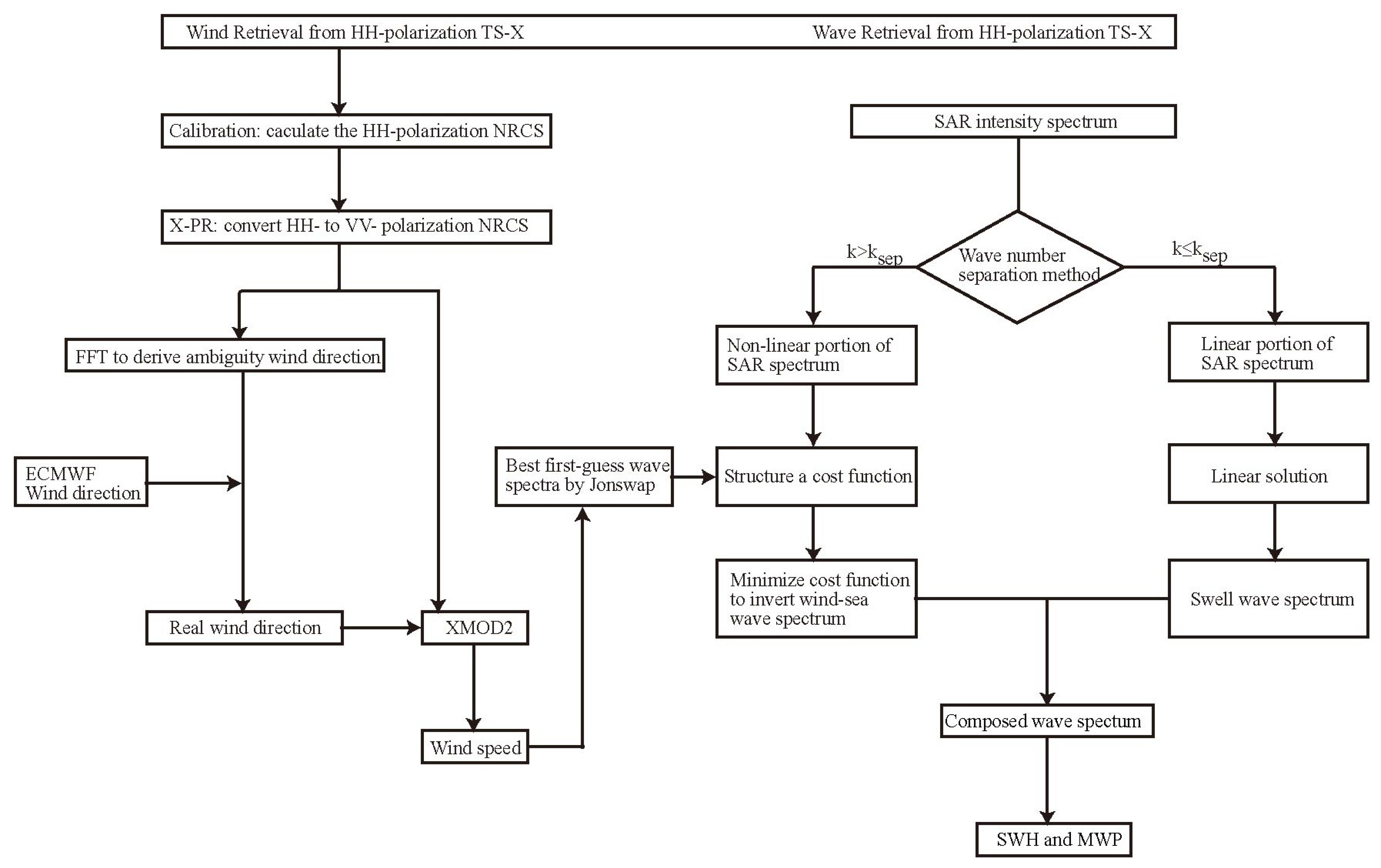
3.3. Scheme of Wave Retrieval Algorithm: PFSM

The PFSM is based on the expression for the forward mapping of a wave spectrum into the SAR image spectrum. Similar to using MPI and SPRA, we need to choose the empirical wave spectrum as the first-guess wave spectrum. The progress in PFSM is that the linear-mapping spectrum portion can be separated from the SAR intensity spectrum by calculating the wavenumber threshold. The threshold is determined by [14]:

$$\left|k_{sep}\right|\approx {(2.87g\frac{V^2}{R^2}\frac{1}{U_{10}^4{\cos }^2\text{φ}({\sin }^2\text{θ}{\sin }^2\text{φ}+{\cos }^2\text{φ})})}^{1/3}$$

(7)

where, V is the satellite platform velocity, R is satellite slant range (definition is the distance between radar and sea surface), g is gravity acceleration, and ϕ is the angle between wave propagation direction and radar look direction. Referring to [14], the portion of the linear-mapping SAR spectrum is where the wave numbers are smaller than the separation wave number |k_sep|, and the left portion corresponds to the non-linear wind–sea state.

The reduction of the non-linear mapping to a linear mapping spectrum for wave numbers less than k_sep means that velocity bunching can be ignored for this regime [26]. Under this condition, the wave spectrum can be inverted directly from the linear part in the SAR spectrum, while for the non-linear part of the SAR spectrum, it is important to search for the most suitable parameters of sea state, including peak phase velocity and wave propagation direction, to produce the first-guess wave spectrum by JONSWAP empirical function. After that, the MPI is applied to invert the wind–sea wave spectrum using the prior best first-guess wave spectrum. Finally, SWH and MWP can be derived from a one-dimension wave number spectrum, combining the wind–sea and swell wave spectra inverted from TS-X. The spectrum of a TS-X intensity image has two peaks. Wave retrieval based on such an image spectrum has an inherent 180° directional ambiguity. We cannot remove the ambiguity without additional external information. However, SWH and MWP can been obtained directly using Equations (8) and (9) from the inverted two-dimensional wave number spectrum, W(k).

$$\text{SWH}=4\cdot \sqrt{{\displaystyle {\int }_0^{\infty }W(k)}dk}$$

(8)

$$\text{MWP}=\frac{m_0}{m_2}=\frac{{\displaystyle {\int }_0^{\infty }W(k)}dk}{{\displaystyle {\int }_0^{\infty }{k}^{2}W(k)}dk}$$

(9)

where m₀ and m₂ represent the zero-order and second-order moment of the variance density spectrum, respectively. The scheme for wind and PFSM-derived wave spectra from HH-polarization TS-X is shown in Figure 2.

Figure 2. Block diagram of PFSM scheme for retrieving wind and wave from HH-polarization TS-X data.

Figure 2. Block diagram of PFSM scheme for retrieving wind and wave from HH-polarization TS-X data.

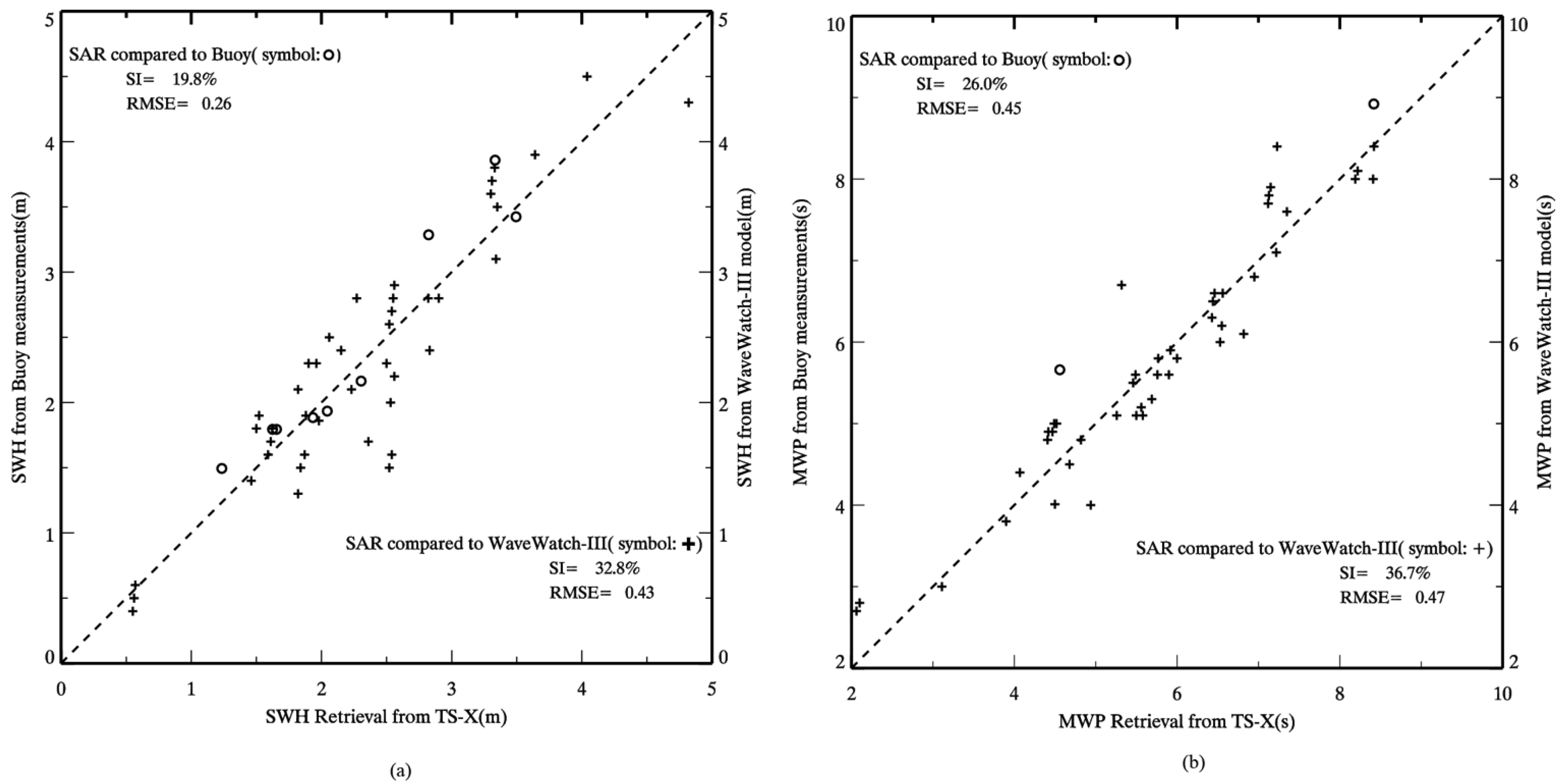
4. SAR Wave Retrieval Validation

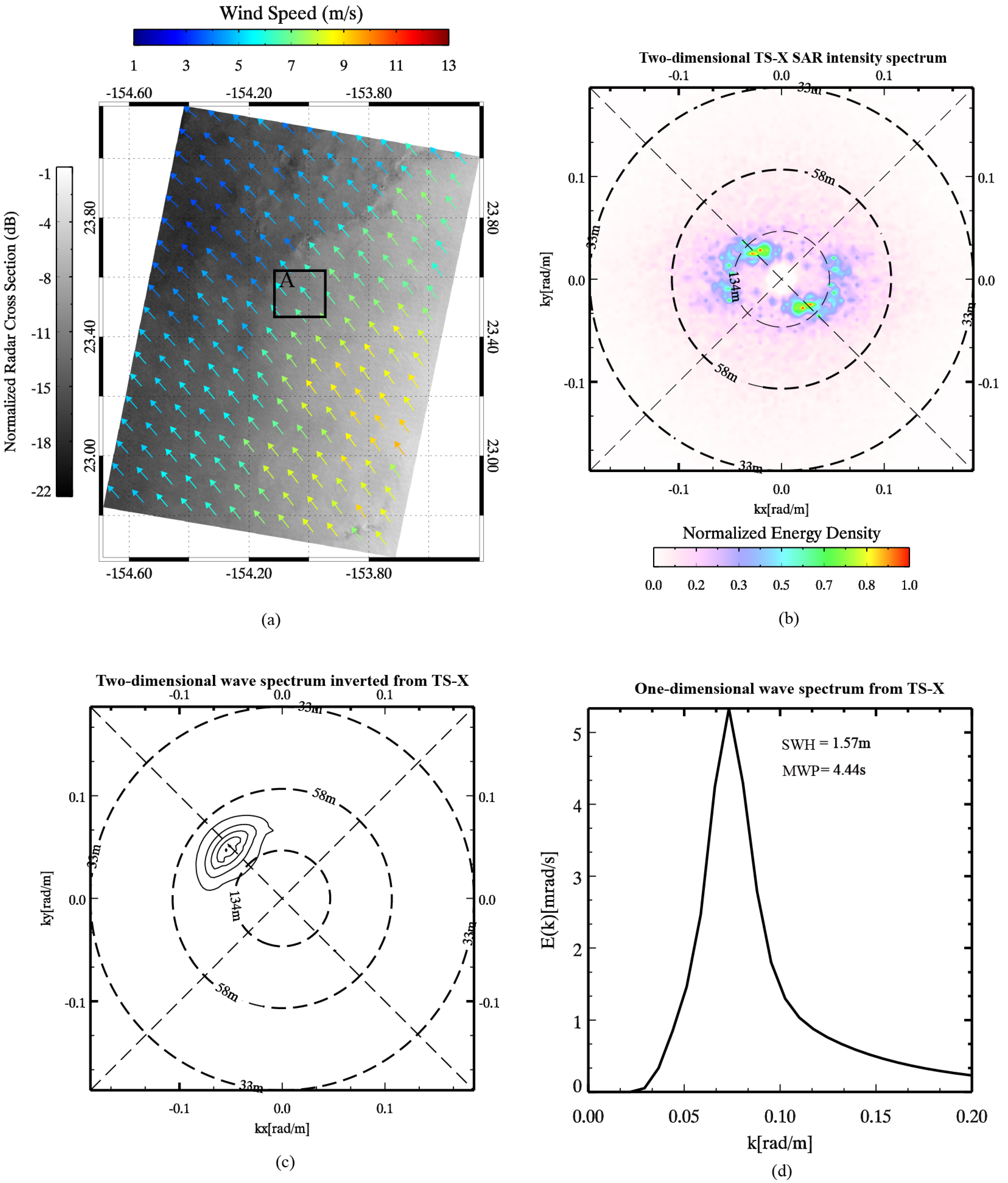
We first show the information retrieved from the SAR image acquired at 4:19 p.m. UTC on 13 December 2010. The SAR wind is shown in Figure 3a. The SAR averaged wind speed in area A centered at the buoy location is 6.5 m/s and the buoy-measured wind is 6.7 m/s. The two-dimensional TS-X SAR intensity spectrum, two-dimensional wave spectrum with corresponding one-dimensional wave spectrum inverted from area A, are shown in Figure 3b–d, respectively, and WAVEWATCH-III computation results are shown in Figure 4. In this case, the ambiguity in the SAR-derived wave direction can be resolved because we can obtain the real wave propagation direction by reference to the wind vector because the wind–sea system in area A is an open sea system far from the land.

However, as for most cases in our study it is impossible to remove the ambiguity in the wind–sea direction because the wave propagation changes a lot due to bathymetry, leading to a mismatch between the SAR-derived wind direction and the 180° ambiguity wave direction from the two-dimensional TS-X intensity spectrum. Although the swell direction has an ambiguity similar to wind–sea, both these have little influence on the inversions of SWH and MWP.

The SAR-derived result of area A in the TS-X, including SWH and MWP, in situ buoy and WAVEWATCH-III computation is shown in Table 3, showing that the relative error of SWH is 15.4% and of MWP is 18.1% compared to the buoy measurement. Furthermore, nine HH-polarization TS-X images covering in situ buoys are processed using the X-band wind GMF and PFSM wave scheme. The SAR and buoy comparison shows that the Root-Mean-Square-Error (RMSE) of SWH is 0.26 m with a Scatter Index (SI) of 19.8% and the RMSE of MWP is 0.45 s with an SI of 26.0%.

Figure 3. A case, taken at 4:19 p.m. UTC on 13 December 2010, showing the wind field and wave retrieval: (a) wind field retrieval; (b) two-dimensional TS-X intensity spectrum; (c) two-dimensional wave spectrum retrieval inverted from TS-X; and (d) one-dimensional wave spectrum retrieval with SWH and MWP.

Figure 3. A case, taken at 4:19 p.m. UTC on 13 December 2010, showing the wind field and wave retrieval: (a) wind field retrieval; (b) two-dimensional TS-X intensity spectrum; (c) two-dimensional wave spectrum retrieval inverted from TS-X; and (d) one-dimensional wave spectrum retrieval with SWH and MWP.

Figure 4. WAVEWATCH-III result of the case, taken at 4:19 p.m. UTC on 13 December 2010, is shown and the black rectangle is the geographic location of TS-X: (a) SWH information and (b) MWP information.

Figure 4. WAVEWATCH-III result of the case, taken at 4:19 p.m. UTC on 13 December 2010, is shown and the black rectangle is the geographic location of TS-X: (a) SWH information and (b) MWP information.

Table 3. The comparison between SAR-derived and in situ buoy measurement, WAVEWATCH-III computation in the area A at 4:19 p.m. UTC on 13 December 2010.

SWH(m) SAR-Derived	MWP(s) SAR-Derived	SWH(m) in situ	MWP(s) in situ	SWH(m) WAVEWATCH-III	MWP(s) WAVEWATCH-III
1.57	4.44	1.82	5.62	2.15	6.8
Bias		−0.25	−1.18	−0.58	−2.36

Table 3. The comparison between SAR-derived and in situ buoy measurement, WAVEWATCH-III computation in the area A at 4:19 p.m. UTC on 13 December 2010.

SWH(m) SAR-Derived	MWP(s) SAR-Derived	SWH(m) in situ	MWP(s) in situ	SWH(m) WAVEWATCH-III	MWP(s) WAVEWATCH-III
1.57	4.44	1.82	5.62	2.15	6.8
Bias		−0.25	−1.18	−0.58	−2.36

In addition, we applied the PFSM algorithm on a total of 16 available TS-X images and compared the results with those from the WAVEWATCH-III model results. In Figure 5a, the RMSE of SWH is 0.43 m with an SI of 32.8% and the RMSE of MWP is 0.47 s with an SI of 34.7%. The wave retrieval has a similar accuracy to that of the C-band SAR, which has an SI of about 20% for SWH when validated against measurements from buoys or altimeters [10,18,27] and an SI of 38% when comparing the wave retrievals with the WAM model predictions [28].

Generally, validation results show that, similar to wave retrieval from C-band SAR, the PFSM is suitable for wave retrieval from HH-polarization X-band SAR data. SAR wave retrieval and in situ buoy measurements comparison show better results than the SAR and WAVEWATCH-III model comparison. According to [29], the non-Bragg contribution produced by wave breaking has a larger impact on HH-polarization than VV-polarization radar signal. Therefore, the PFSM tends to have a better performance for wave retrieval in VV polarization due to less distortion from wave breaking [30,31].

Figure 5. Wave parameters retrieval results from HH-polarization TS-X images are compared to buoy measurements in Table 2 and all TS-X images are compared to computation from the WAVEWATCH-III model: (a) SWH comparison and (b) MWP comparison.

Figure 5. Wave parameters retrieval results from HH-polarization TS-X images are compared to buoy measurements in Table 2 and all TS-X images are compared to computation from the WAVEWATCH-III model: (a) SWH comparison and (b) MWP comparison.

5. Conclusions

In this paper, the algorithm PFSM has been applied to X-band SAR to estimate wave parameters, including SWH and MWP, from the HH-polarization TS-X SAR imagery. Results indicate that the theoretical-based algorithm PFSM, which is developed on the imaging mechanism of waves, provides another way for wave inversion in addition to the empirical algorithm XWAVE.

One case study using the TS-X image acquired on 13 December 2010 is shown. Nine TS-X covering in situ buoys were selected to validate the PFSM algorithm. The RMSE of SWH is 0.26 m with an SI of 19.8% and the RMSE of the MWP is 0.45 s with an SI of 26.0%. A total of 16 TS-X images in HH-polarization were collected for validation against results from the WAVEWATCH-III model, showing that the RMSE of SWH between SAR-derived SWH and the WAVEWATCH-III model computation is 0.43 m with an SI of 32.8% and the RMSE of the MWP is 0.47 s with an SI of 34.7%. An SI of 38% [28] for SWH was found after comparing the estimations from SIR-C SAR with WAM numeric computations. The slightly larger error for model comparison is supposed to be caused by the deficiency of the numeric ocean model [32] and the explicit error of wind retrieval GMF-XMOD2 used together with the X-PR shown in Table 2. It is widely accepted that the SI of SWH from C-band SAR is around 20% compared to buoy measurements [18]. Although this study shows that the PFSM ocean wave retrieval algorithm achieves an SI of SWH within 20% for HH-polarization X-band SAR data against in situ buoys, we think that the algorithm would perform better for VV-polarization because the non-Bragg contribution on radar backscatter at VV-polarization is smaller than that at HH-polarization [30].

References

1. Li, X.M.; Lehner, S. Algorithm for sea surface wind retrieval from TerraSAR-X and TanDEM-X Data. IEEE Trans. Geosci. Remote Sens. 2014, 52, 2928–2939. [Google Scholar]
2. Ren, Y.Z.; He, M.X.; Lehner, S. An algorithm for the retrieval of sea surface wind fields using X-band TerraSAR-X data. Int. J. Remote Sens. 2012, 33, 7310–7336. [Google Scholar] [CrossRef]
3. Shao, W.Z.; Li, X.M.; Lehner, S.; Guan, C.L. Development of Polarization Ratio model for sea surface wind field retrieval from TerraSAR-X HH polarization data. Int. J. Remote Sens. 2014, 35, 4046–4063. [Google Scholar] [CrossRef]
4. Alpers, W.; Ross, D.B.; Rufenach, C.L. On the detectability of ocean surface waves by real and synthetic radar. J. Geophys. Res. 1981, 86, 10529–10546. [Google Scholar] [CrossRef]
5. Hasselmann, S.; Hasselmann, K. Computations and parametrizations of the nonlinear energy transfer in a gravity-wave spectrum. I: A new method for efficient computations of the exact nonlinear transfer integral. J. Phys. Oceanogr. 1985, 15, 1369–1377. [Google Scholar] [CrossRef]
6. Alpers, W.; Bruning, C. On the relative importance of motion-related contributions to SAR imaging mechanism of ocean surface waves. IEEE Trans. Geosci. Remote Sens. 1986, 24, 873–885. [Google Scholar] [CrossRef]
7. Li, X.F.; Pichel, W.; He, M.; Wu, S.; Friedman, K.; Clemente-Colon, P.; Zhao, C. Observation of hurricane-generated ocean swell refraction at the Gulf Stream North Wall with the RADARSAT-1 synthetic aperture radar. IEEE Trans. Geosci. Remote Sens. 2002, 40, 2131–2142. [Google Scholar]
8. Hasselmann, K.; Hasselmann, S. On the nonlinear mapping of an ocean wave spectrum into a synthetic aperture radar image spectrum. J. Geophys. Res. 1991, 96, 10713–10729. [Google Scholar] [CrossRef]
9. Hasselmann, S.; Bruning, C.; Hasselmann, K. An improved algorithm for the retrieval of ocean wave spectra from synthetic aperture radar image spectra. J. Geophys. Res. 1996, 101, 6615–6629. [Google Scholar] [CrossRef]
10. Schulz-Stellenfleth, J.; Lehner, S.; Hoja, D. A parametric scheme for the retrieval of two-dimensional ocean wave spectra from synthetic aperture radar look cross spectra. J. Geophys. Res. 2005, 110, 97–314. [Google Scholar] [CrossRef]
11. Mastenbroek, C.; de Valk, C.F. A semi-parametric algorithm to retrieve ocean wave spectra from synthetic aperture radar. J. Geophys. Res. 2000, 105, 3497–3516. [Google Scholar] [CrossRef]
12. Hasselmann, K.; Barnett, T.P.; Bouws, E.; Carlson, H.; Cartwright, D.E.; Enke, K.; Ewing, J.A.; Gienapp, H.; Hasselmann, D.E.; Kruseman, P.; et al. Measurements of Wind-Wave Growth and Swell Decay during the Joint North Sea Wave Project (JONSWAP); UDC 551.466.31; Deutches Hydrographisches Institut: Hamburg, Germany, 1973. [Google Scholar]
13. Voorrips, C.; Makin, V.; Hasselmann, S. Assimilation of wave spectra from pitch-and-roll buoys in a North Sea wave model. J. Geophys. Res. 1997, 102, 5829–5849. [Google Scholar] [CrossRef]
14. Sun, J.; Guan, C.L. Parameterized first-guess spectrum method for retrieving directional spectrum of swell-dominated waves and huge waves from SAR images. Chin. J. Oceanol. Limnol. 2006, 24, 12–20. [Google Scholar]
15. Sun, J.; Kawamura, H. Retrieval of surface wave parameters from SAR images and their validation in the coastal seas around Japan. J. Oceanogr. 2009, 65, 567–577. [Google Scholar] [CrossRef]
16. Schulz-Stellenfleth, J.; Konig, T.; Lehner, S. An empirical approach for the retrieval of integral ocean wave parameters from synthetic aperture radar data. J. Geophys. Res. 2007, 112, 1–14. [Google Scholar]
17. Li, X.M.; Lehner, S.; Rosenthal, W. Investigation of ocean surface wave refraction using TerraSAR-X data. IEEE Trans. Geosci. Remote Sens. 2010, 48, 830–840. [Google Scholar]
18. Li, X.M.; Lehner, S.; Bruns, T. Ocean wave integral parameter measurements using Envisat ASAR wave mode data. IEEE Trans. Geosci. Remote Sens. 2011, 49, 155–174. [Google Scholar] [CrossRef]
19. Bruck, M.; Lehner, S. Coastal wave field extraction using TerraSAR-X data. J. Appl. Remote Sens. 2013. [Google Scholar] [CrossRef]
20. Yang, X.F.; Li, X.F.; Pichel, W.; Li, Z.W. Comparison of ocean surface winds from ENVISAT ASAR, MetOp ASCAT scatterometer, buoy measurements, and NOGAPS model. IEEE Trans. Geosci. Remote Sens. 2011, 49, 4743–4750. [Google Scholar] [CrossRef]
21. Wackerman, C.; Clemente-Colon, P.; Pichel, W.; Li, X. A two-scale model to predict C-band VV and HH normalized radar cross section values over the ocean. Can. J. Remote Sens. 2002, 28, 367–384. [Google Scholar]
22. Yang, X.; Li, X.; Zheng, Q.; Gu, X.; Pichel, W.; Li, Z.W. Comparison of ocean-surface winds retrieved from QuikSCAT scatterometer and Radarsat-1 SAR in offshore waters of the U.S. west coast. IEEE Geosci. Remote Sens. Lett. 2011, 8, 163–167. [Google Scholar] [CrossRef]
23. Xu, Q.; Lin, H.; Li, X.F.; Zheng, Q.; Pichel, W.; Liu, Y. Assessment of an analytical model for sea surface wind speed retrieval from spaceborne SAR. Int. J. Remote Sens. 2010, 31, 993–1008. [Google Scholar]
24. Zhang, B.; Li, X.; Perrie, W.; He, Y. Synergistic measurements of ocean winds and waves from SAR. J. Geophys. Res. 2015. [Google Scholar] [CrossRef]
25. Tolman, H.L. A mosaic approach to wind wave modeling. Ocean Model. 2008, 25, 35–47. [Google Scholar] [CrossRef]
26. Alpers, W.; Rufenach, C. The effect of orbital motions on synthetic aperture radar imagery of ocean waves. IEEE Trans. Antenn. Propag. 1979, 27, 685–690. [Google Scholar] [CrossRef]
27. Wang, H.; Zhu, J.; Yang, J. A semiempirical algorithm for SAR wave height retrieval and its validation using Envisat ASAR wave mode data. Acta Oceanol. Sin. 2012, 31, 59–66. [Google Scholar] [CrossRef]
28. Monaldo, F.M.; Beal, R.C. Comparison of SIR-C SAR wavenumber spectra with WAM model predictions. J. Geophys. Res. 1998, 103, 18815–18825. [Google Scholar] [CrossRef]
29. Kudryavtsev, V.; Hauser, D.; Caudal, G.; Chapron, B. A semiempirical model of the normalized radar cross section of the sea surface, 2. Radar modulation transfer function. J. Geophys. Res. 2003, 108. [Google Scholar] [CrossRef]
30. Phillips, O.M.; Posner, F.L.; Hansen, J.P. High range resolution radar measurements of the speed distribution of breaking events in wind-generated ocean waves: Surface impulse and wave energy dissipation rates. J. Phys. Oceanogr. 2001, 31, 450–460. [Google Scholar] [CrossRef]
31. Haller, M.C.; Lyzenga, D.R. Comparison of radar and video observations of shallow water breaking waves. IEEE Geosci. Remote Sens. Lett. 2003, 41, 832–844. [Google Scholar] [CrossRef]
32. Cavaleri, L. Wave modeling—Missing the peaks. J. Phys. Oceanogr. 2009, 39, 2757–2778. [Google Scholar] [CrossRef]