
Metadata-Assisted Global Motion Estimation for Medium-Altitude Unmanned Aerial Vehicle Video Applications

Abstract
:
1. Introduction
1.1. Background
1.1.1. Unmanned Aerial Vehicle Remote Sensing
1.1.2. Utility of Global Motion Estimation in UAVRS

| Key Technology | Video Processing of UAV Vision | Applications in UAVRS |
|---|---|---|
| GME | Video encoding | Data acquisition |
| Video stabilization | Data acquisition | |
| Target detection and tracking | Target monitoring and surveillance | |
| Video shot segmentation and retrieval | Data retrieval and production from a video database | |
| Super-resolution reconstruction | Crop and forest monitoring, change detection | |
| Structure from motion | 3D reconstruction and 3D mapping for disaster areas |
1.1.3. Problems in GME
- (1)
- How to improve precision under a large-scale motion condition?
- (2)
- How to reduce the dependence on image information to adapt to several special landforms?
- (3)
- How to enhance adaptability to different UAVs?
1.2. Related Work
- (1)
- The research objects were predominantly small, and low-altitude UAVs that have different structures were employed. This condition leads to poor expansibility of the method.
- (2)
- The information used was not the bottom data measured from the UAV system, and some information was assumed to be known. Thus, the process of GME was not completed from the bottom level.
- (3)
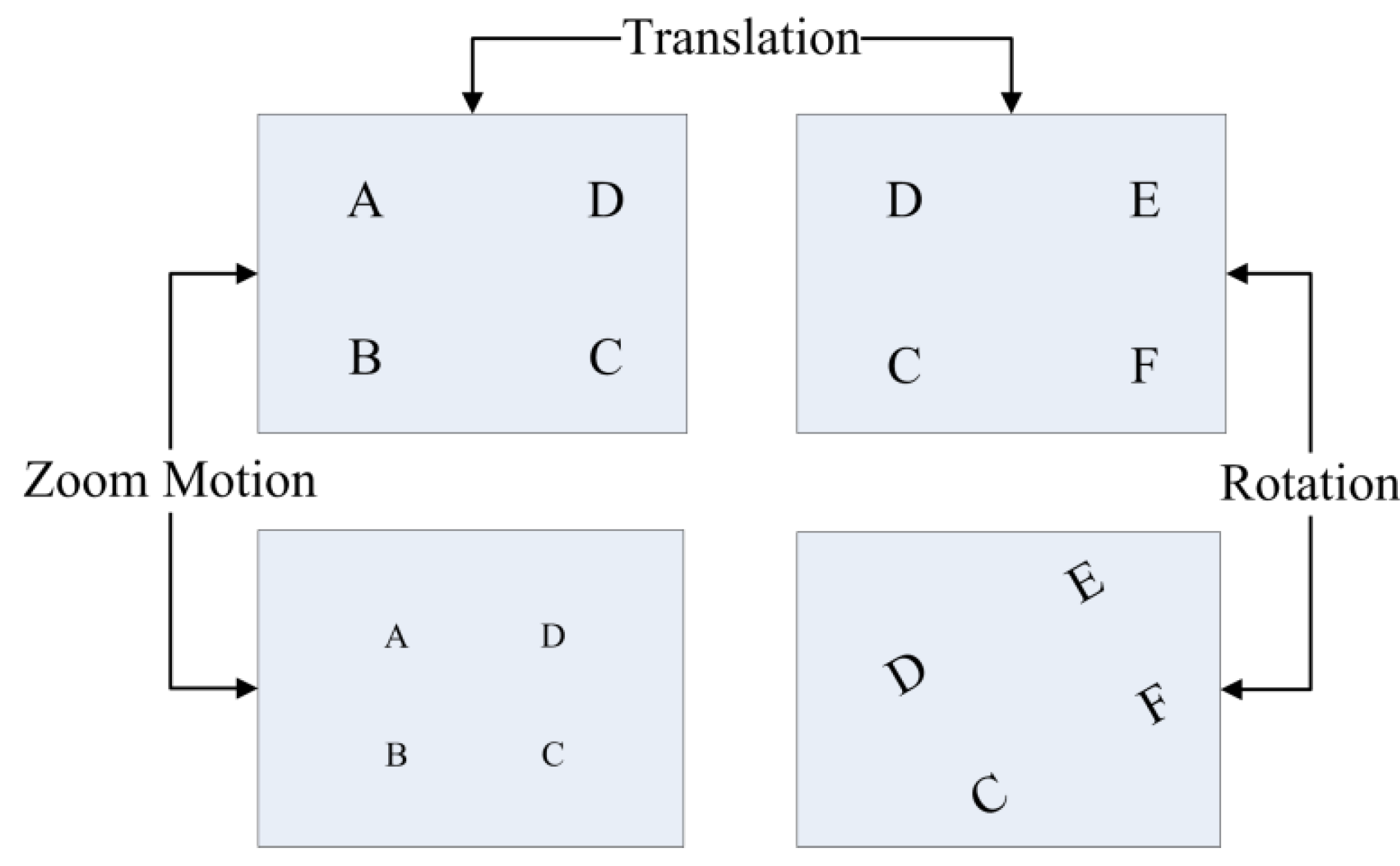
- The motion of the dual platform was often assumed to be smooth and stable, which confines GME to a narrow baseline condition. However, even the same contents (e.g., house, bridges) of two adjacent frames differ in geometric features (shape and size), location, and orientation when the vehicle’s translation or the dual platform’s behavior changes considerably.
1.3. Present Work
2. Methodology
2.1. Scheme of Metadata-Assisted GME
2.1.1. Study Hypotheses
2.1.2. Metadata
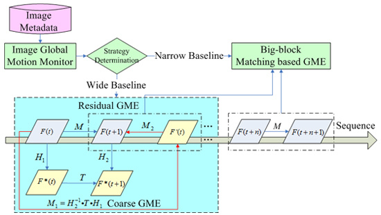
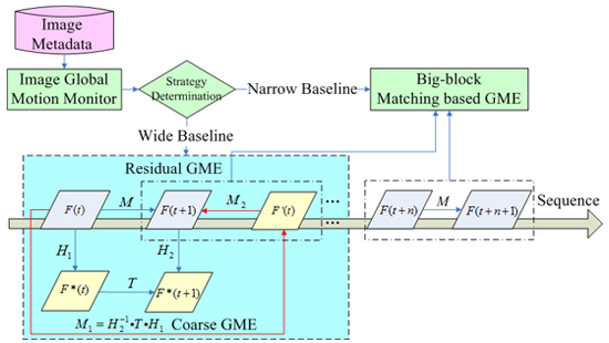
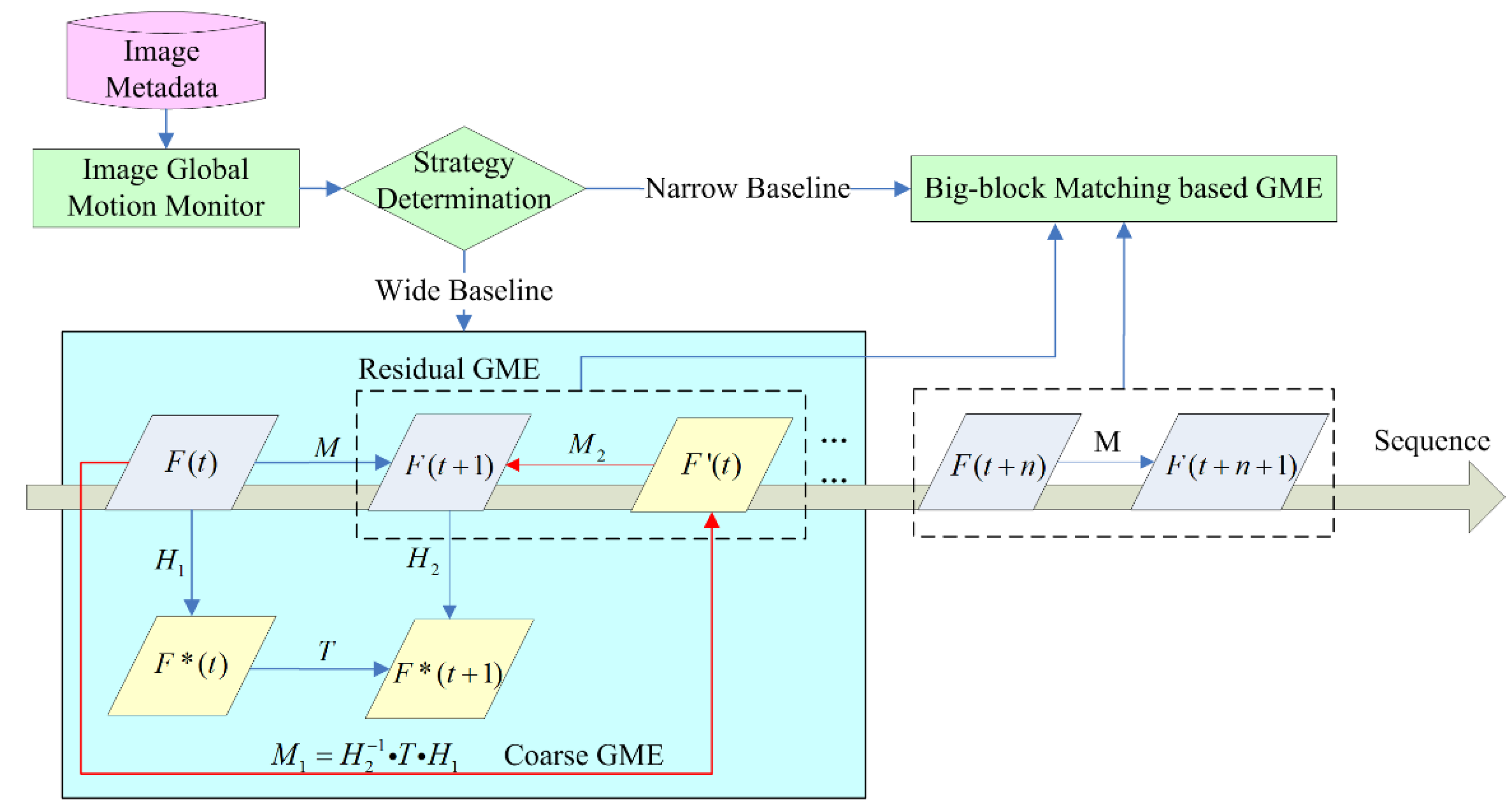
2.1.3. Workflow of MaGME
| Index | Name | Notation | Description |
|---|---|---|---|
| 1 | Longitude | Lng | Measured by GPS, unit: degree |
| 2 | Latitude | Lat | Measured by GPS, unit: degree |
| 3 | Altitude | Alt | Measured by altimeter, unit: meter |
| 4 | Terrain height | Ter | Obtained from GIS, unit: meter |
| 5 | Vehicle heading | H | Angle between the UAV’s nose and the North measured by INS, unit: degree |
| 6 | Vehicle roll | R | Measured by INS, unit: degree |
| 7 | Vehicle pitch | P | Measured by INS, unit: degree |
| 8–10 | Camera installation Translation | tCX、 tCY、 tCZ | Translation from camera to GPS on X-, Y-, and Z-axes, unit: meter |
| 11 | Camera pan | pan | Angle between the camera’s optical axis and the UAV’s nose, unit: degree |
| 12 | Camera tilt | tilt | Angle between the camera’s optical axis and the UAV body plane, unit: degree |
| 13 | Resolution | Row*Col | Row: image row, Col: image column |
| 14 | Focal length | f | Unit: meter |
| 15 | Pixel size | u | Size of each pixel, unit: meter |

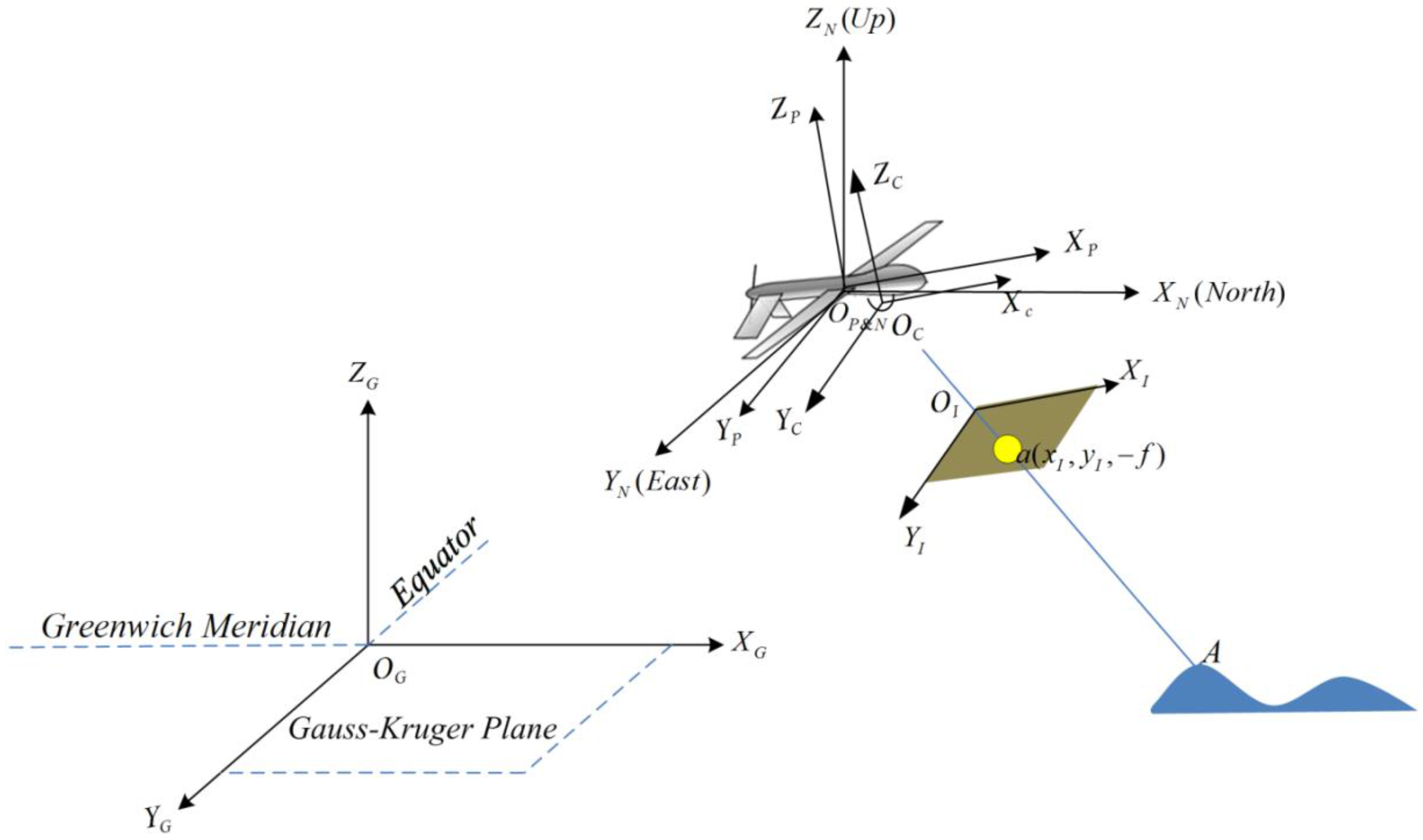
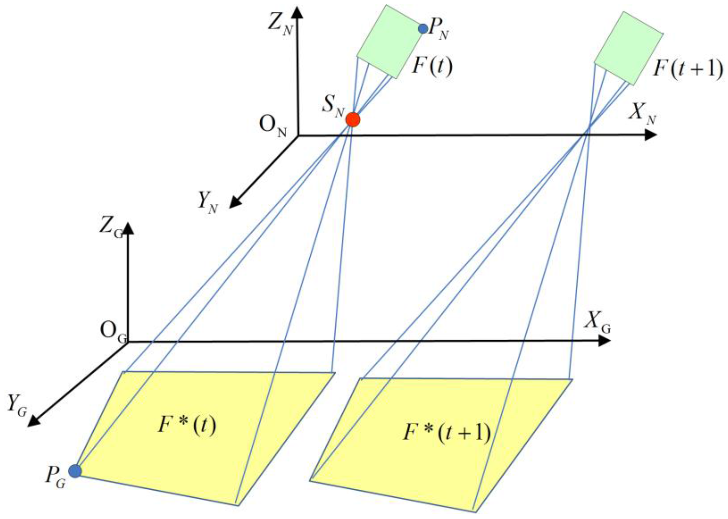
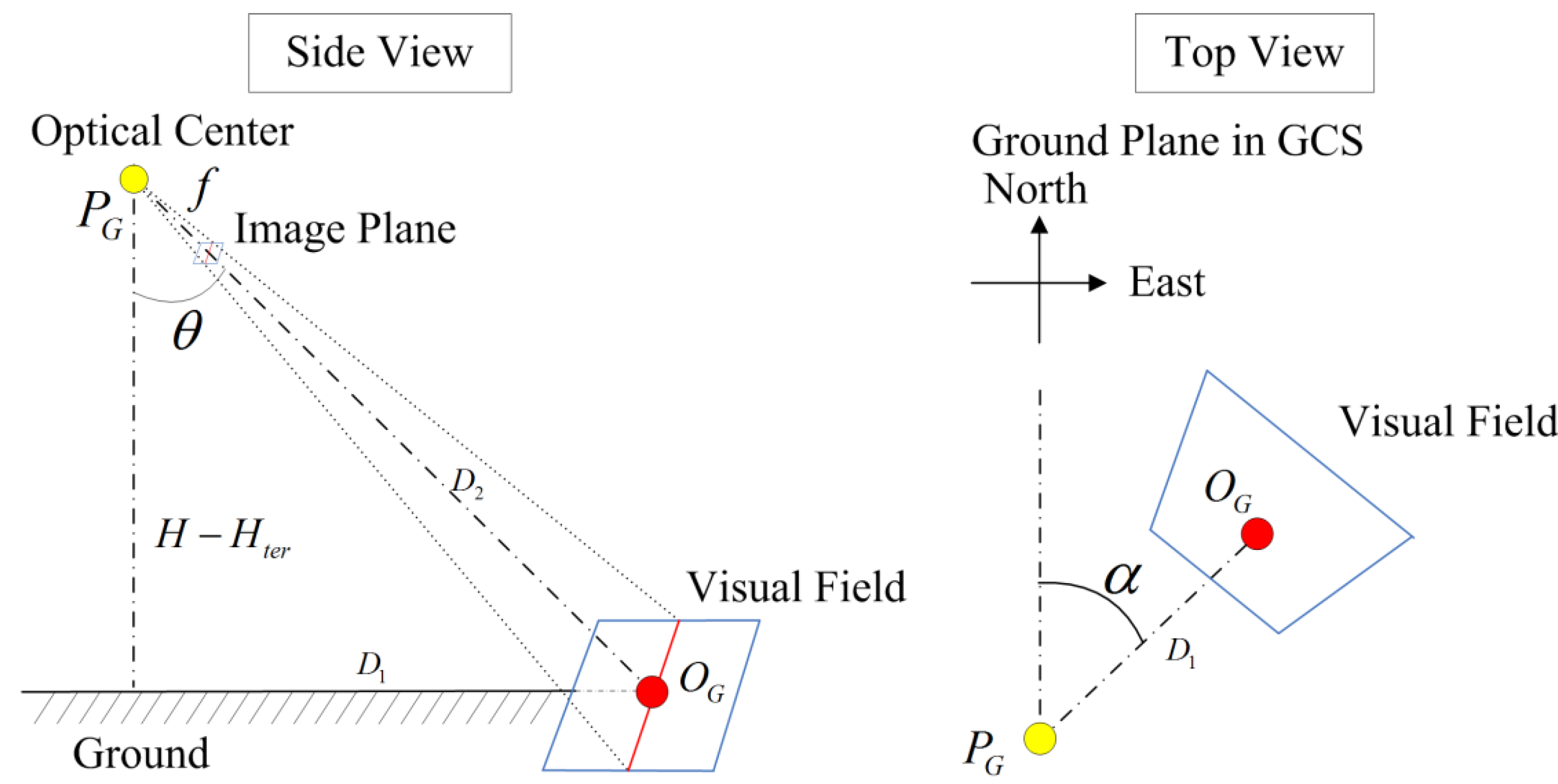
2.2. Coordinate Transformation

| Transformation | Description |
|---|---|
| Translation from ICS to CCS; and are equal to the half of the physical width and height of the imaging plane in value | |
| Translation from CCS to PCS; , , and are the three translations on X-, Y-, and Z-axes | |
| Projective projection from CCS to PCS; two DOFs: pan and tilt | |
| Projective projection from PCS to NCS; h: heading, p: pitch, r: roll | |
| Translation from NCS to GCS; , , and are the three translations on X-, Y-, and Z-axes |
2.3. Coarse GME

2.4. Residual GME
2.4.1. Information and Contrast Feature
2.4.2. Residual GME Based on Big-block Matching

2.5. Image Motion Monitor
3. Results and Discussion
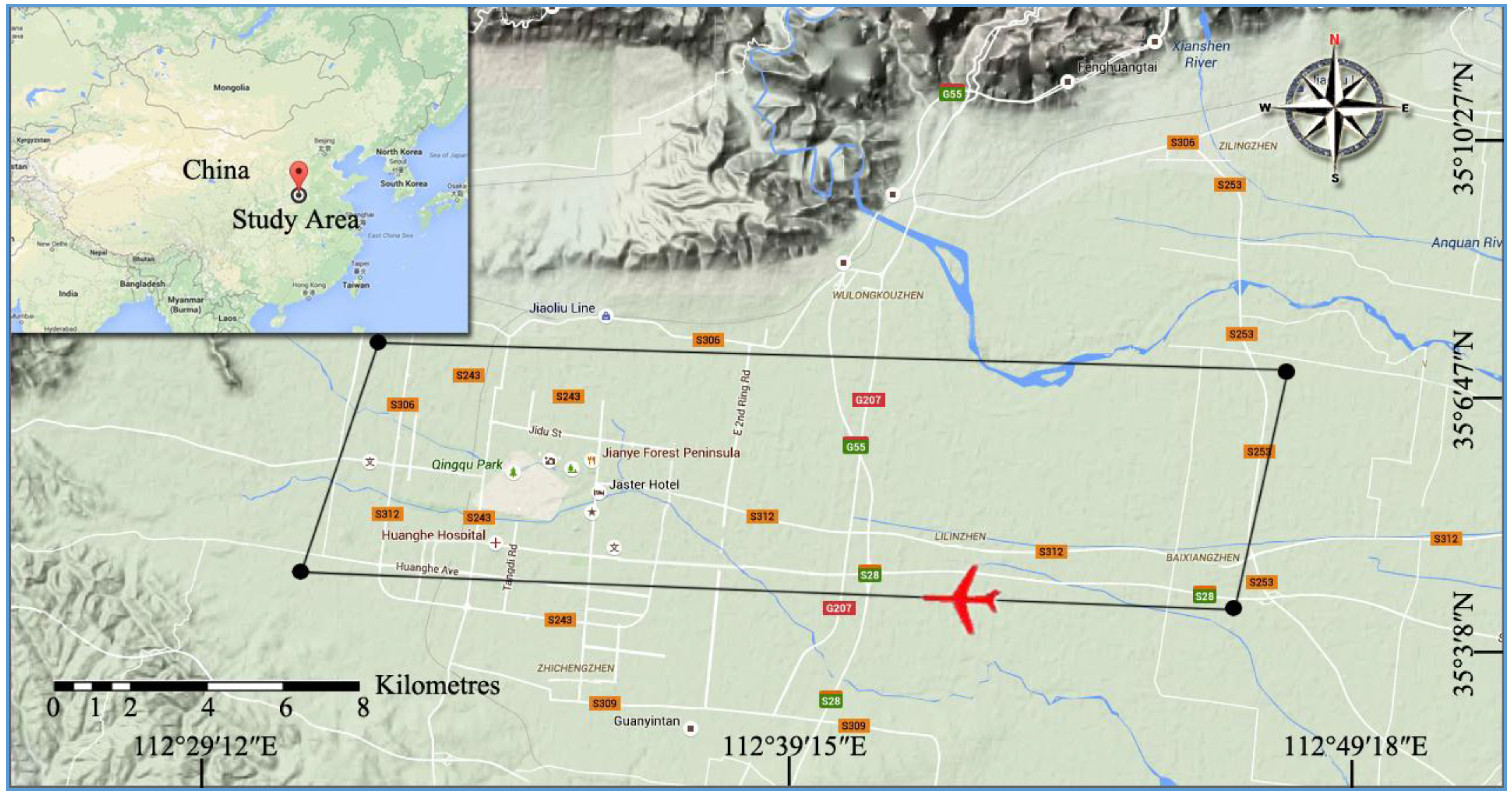
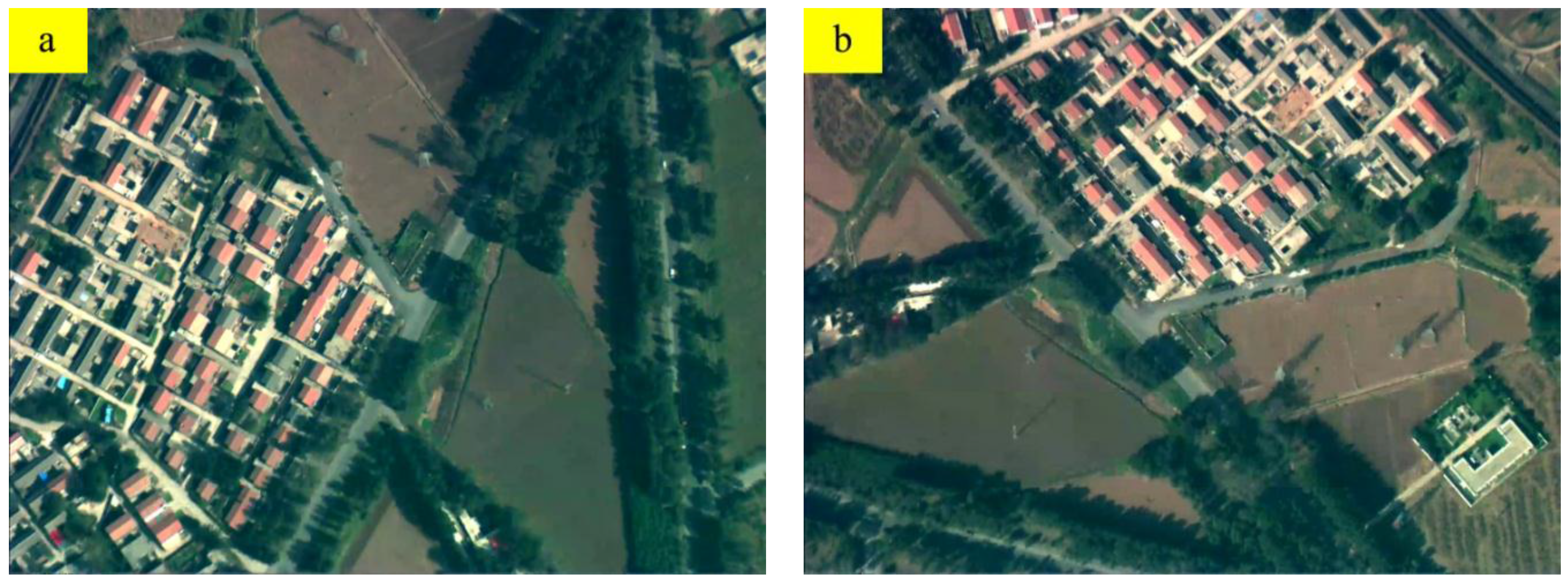
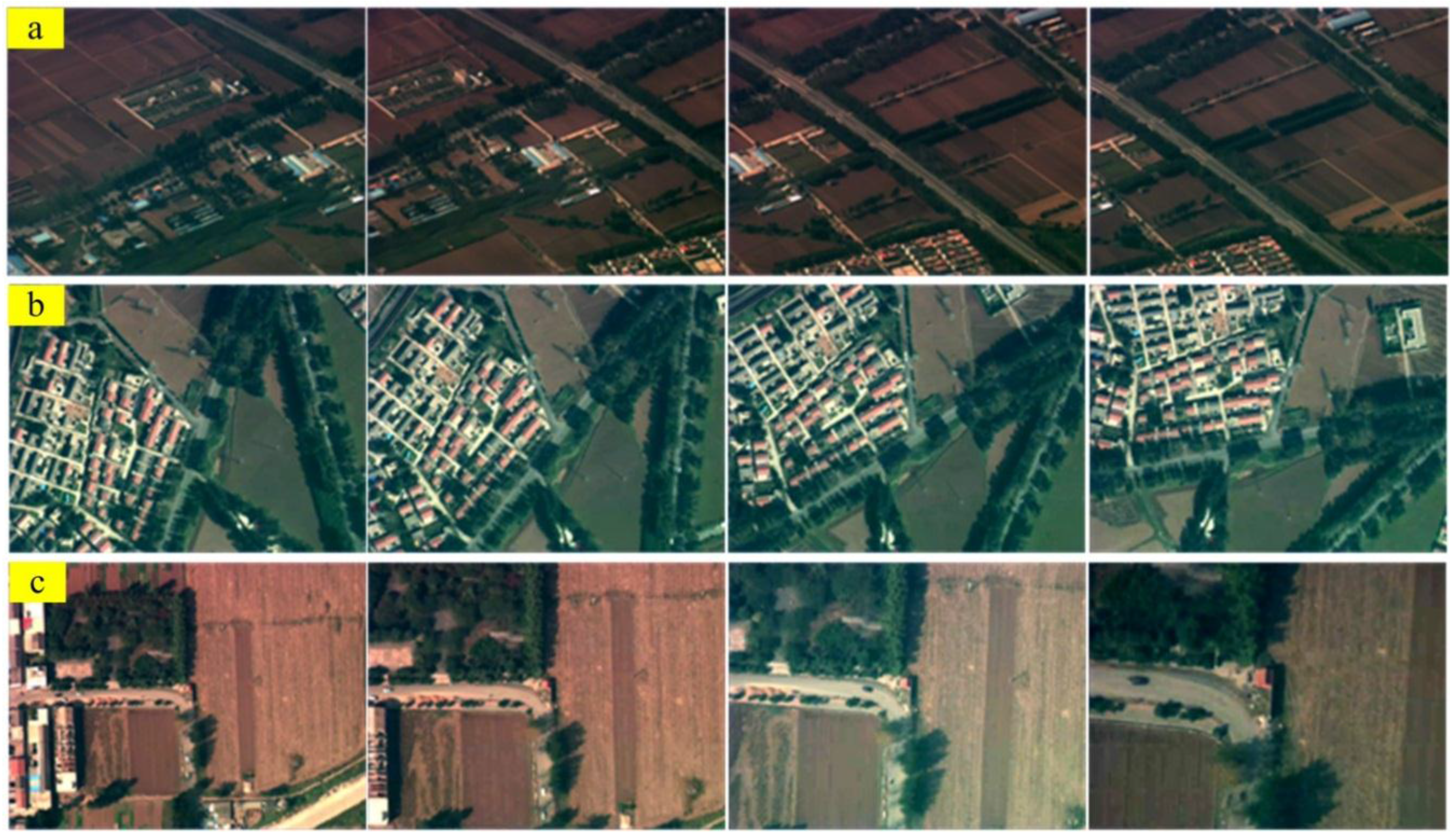
3.1. Study Area and Dataset

3.2. Coarse GME


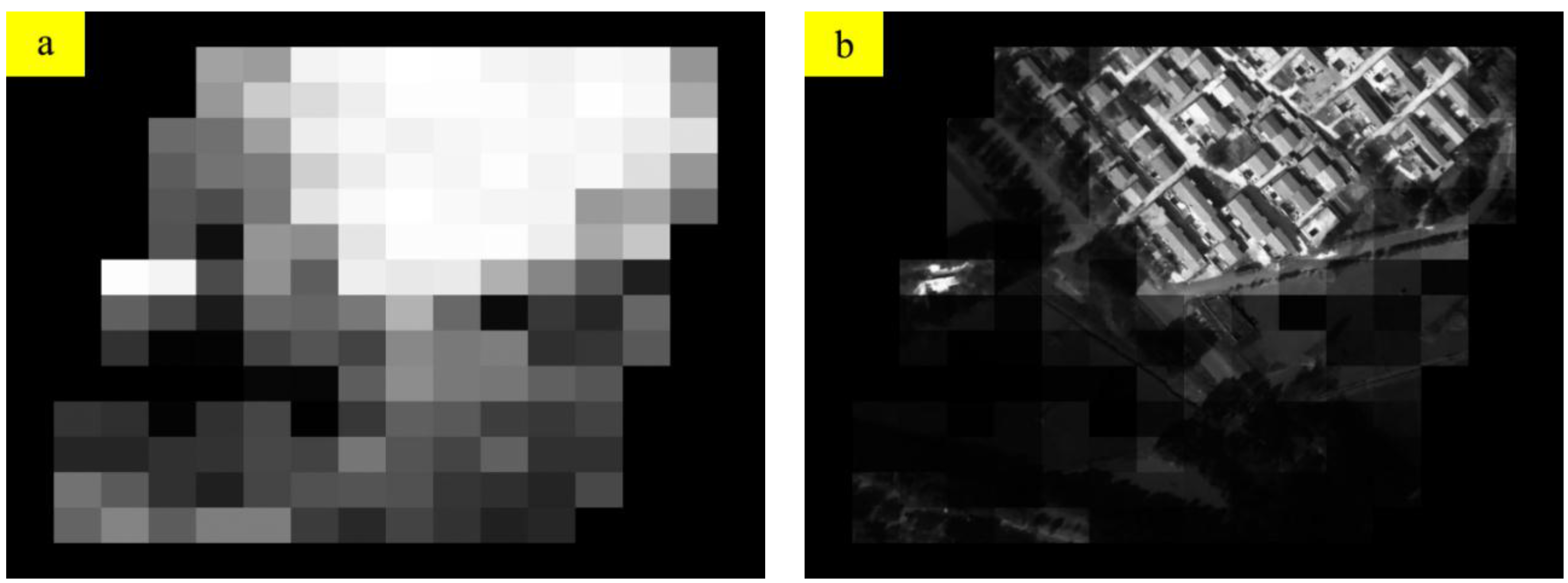
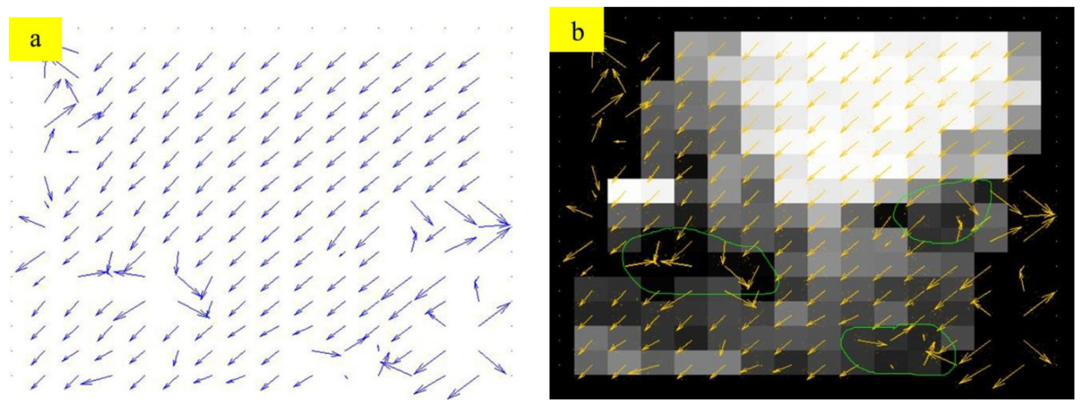
3.3. Residual GME


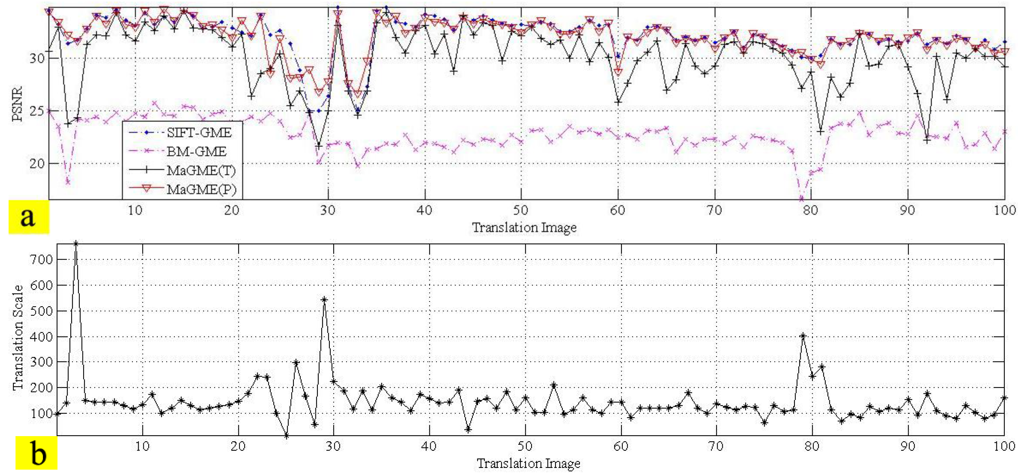
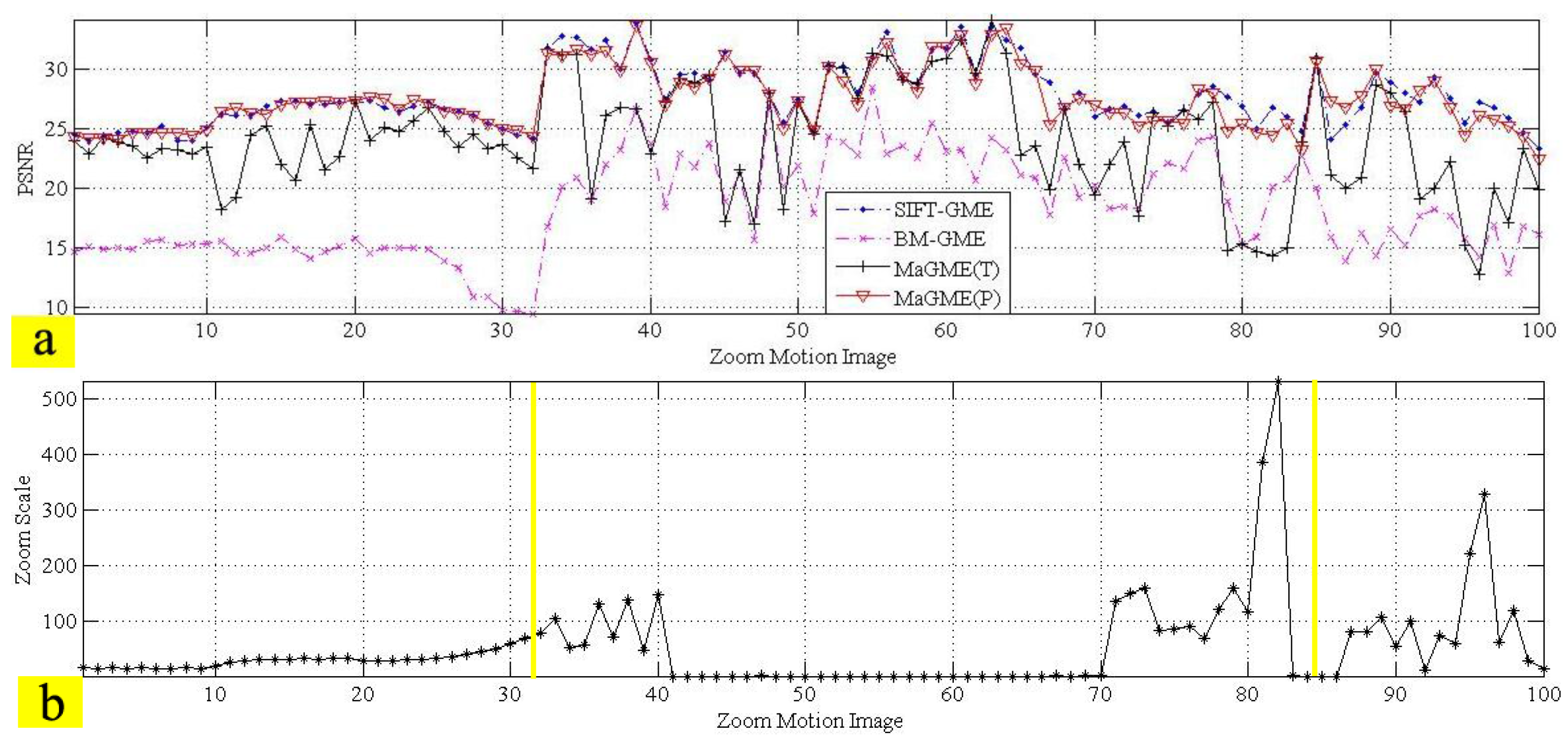
3.4. Performance of the Entire Algorithm

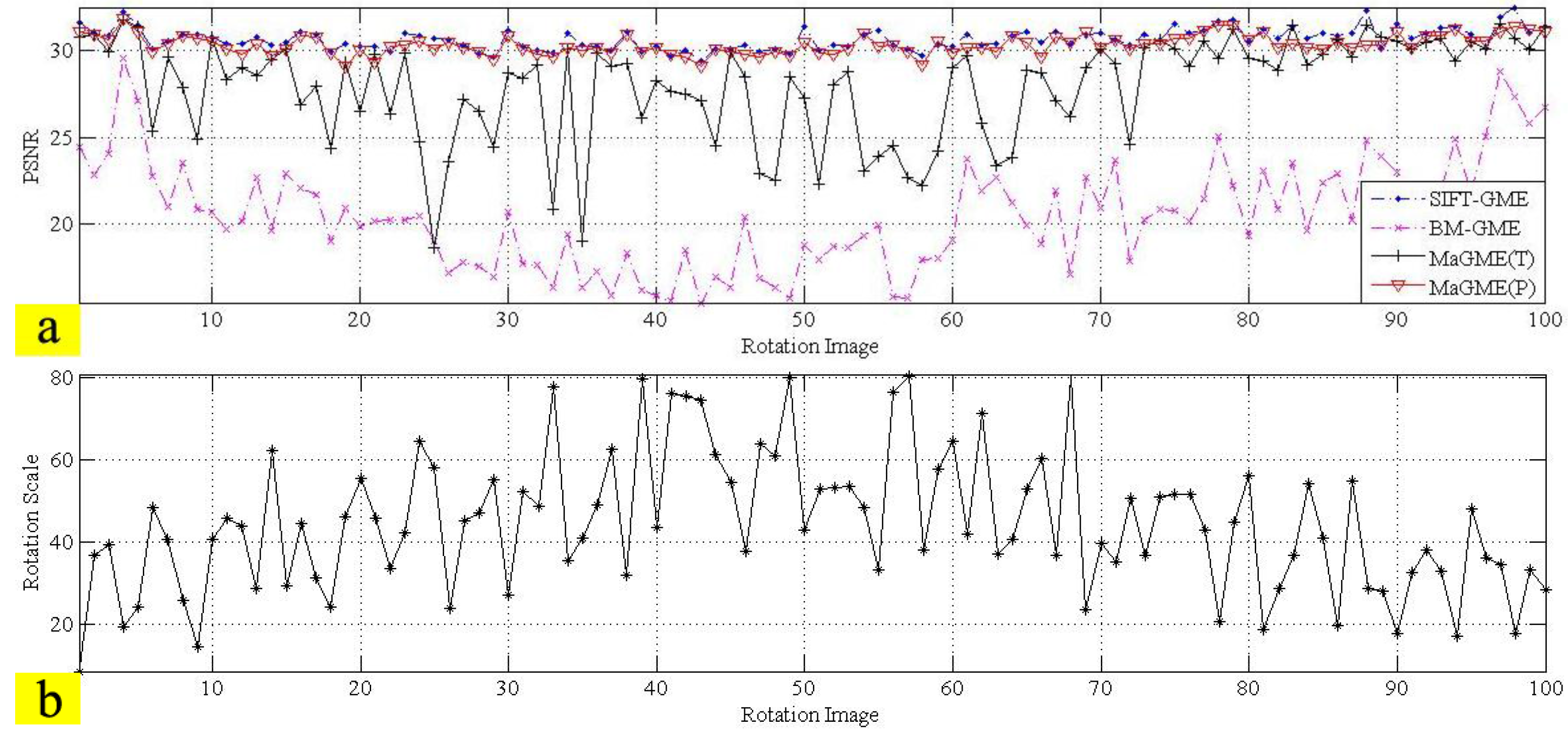

| Test Sequence (Frame Number) | SIFT-GME Average PSNR (dB) | BM-GME Average PSNR (dB) | MaGME(T) Average PSNR (dB) | MaGME(P)Average PSNR (dB) |
|---|---|---|---|---|
| Translation (100) | 32.18 | 22.77 | 30.10 | 32.09 |
| Rotation (100) | 30.70 | 20.49 | 27.94 | 30.36 |
| Zoom motion (100) | 27.67 | 18.22 | 24.01 | 27.37 |
| Average PSNR | 30.18 | 20.49 | 27.35 | 29.94 |
4. Conclusions
Acknowledgements
Author Contributions
Conflicts of Interest
References
- Pajares, G. Overview and current status of remote sensing applications based on unmanned aerial vehicles (UAVs). J. Photogramm. Eng. Remote Sens. 2015, 81, 281–329. [Google Scholar] [CrossRef]
- Vachtsevanos, G.J.; Valavanis, K.P. Military and civilian unmanned aircraft. In Handbook of Unmanned Aerial Vehicles; Valavanis, K.P., Vachtsevanos, G.J., Eds.; Springer Netherlands: Berlin, Germany, 2015; pp. 93–103. [Google Scholar]
- Toma, A. Use of Unmanned Aerial Systems in Civil Applications. Ph.D. Thesis, Politecnico di Torino, Torino, Italy, 2015. [Google Scholar]
- D’Oleire-Oltmanns, S.; Marzolff, I.; Peter, K.D.; Ries, J.B. Unmanned aerial vehicle (UAV) for monitoring soil erosion in Morocco. Remote Sens. 2012, 4, 3390–3416. [Google Scholar] [CrossRef]
- Tong, X.H.; Liu, X.F.; Chen, P.; Liu, S.J.; Luan, K.F.; Li, L.Y.; Liu, S.; Liu, X.L.; Xie, H.; Jin, Y.M.; et al. Integration of UAV-based photogrammetry and terrestrial Laser scanning for the three-dimensional mapping and monitoring of open-pit mine areas. Remote Sens. 2015, 7, 6635–6662. [Google Scholar] [CrossRef]
- Bendig, J.; Bolten, A.; Bennertz, S.; Broscheit, J.; Eichfuss, S.; Bareth, G. Estimating biomass of barley using crop surface models (CSMs) derived from UAV-based RGB imaging. Remote Sens. 2014, 6, 10395–10412. [Google Scholar] [CrossRef]
- Getzin, S.; Nuske, R.; Wiegand, K. Using unmanned aerial vehicles (UAV) to quantify spatial gap patterns in forests. Remote Sens. 2014, 6, 6988–7004. [Google Scholar] [CrossRef]
- Towler, J.; Krawiec, B.; Kochersberger, K. Radiation mapping in post-disaster environments using an autonomous helicopter. Remote Sens. 2012, 4, 1995–2015. [Google Scholar] [CrossRef]
- Skoglar, P.; Orguner, U.; Törnqvist, D.; Gustafsson, F. Road target search and tracking with gimbaled vision sensor on an unmanned aerial vehicle. Remote Sens. 2012, 4, 2076–2111. [Google Scholar] [CrossRef]
- Watts, A.; Ambrosia, V.; Hinkley, E. Unmanned aircraft systems in remote sensing and scientific research: Classification and considerations of use. Remote Sens. 2012, 4, 1671–1692. [Google Scholar] [CrossRef]
- Kendoul, F. Survey of advances in guidance, navigation, and control of unmanned rotorcraft systems. J. Field Robot. 2012, 29, 315–378. [Google Scholar] [CrossRef]
- Mai, Y.; Zhao, H.; Guo, S. The analysis of image stabilization technology based on small-UAV airborne video. In Proceedings of International Conference on Computer Science & Electronics Engineering, Hangzhou, China, 23–25 March 2012; pp. 586–589.
- Brockers, R.; Humenberger, M.; Kuwata, Y.; Matthies, L.; Weiss, S. Computer vision for micro air vehicles. In Advances in Computer Vision & Pattern Recognition; Kisačanin, B., Gelautz, M., Eds.; Springer International Publishing: Berlin, Germany, 2014; pp. 73–107. [Google Scholar]
- Kanade, T.; Amidi, O.; Ke, Q. Real-Time and 3D Vision for Autonomous Small and Micro Air Vehicles. Available online: http://www.cs.cmu.edu/~ke/publications/ke_CDC_04_AUV.pdf (accessed on 5 July 2015).
- Wang, Y.; Hou, Z.; Leman, K.; Chang, R. Real-Time Video Stabilization for Unmanned Aerial Vehicles. Available online: http://www1.i2r.a-star.edu.sg/~ywang/papers/MVA_2011_Real-Time%20Video%20Stabilization%20for%20Unmanned%20Aerial%20Vehicles.pdf (accessed on 5 July 2015).
- Bhaskaranand, M.; Gibson, J.D. Low-complexity video encoding for UAV reconnaissance and surveillance. In Proceedings of Military Communications IEEE Conference, Baltimore, MD, USA, 7–10 November 2011; pp. 1633–1638.
- Rodríguez-Canosa, G.R.; Thomas, S.; del Cerro, J.; Barrientos, A.; MacDonald, B. A real-time method to detect and track moving objects (DATMO) from unmanned aerial vehicles (UAVs) using a single camera. Remote Sens. 2012, 4, 1090–1111. [Google Scholar] [CrossRef]
- Hsieh, J.; Yu, S.; Chen, Y. Motion-based video retrieval by trajectory matching. IEEE Trans. Circuits Syst. Video Technol. 2006, 16, 396–409. [Google Scholar]
- Zhang, H.; Yang, Z.; Zhang, L.; Shen, H. Super-resolution reconstruction for multi-angle remote sensing images considering resolution differences. Remote Sens. 2014, 6, 637–657. [Google Scholar] [CrossRef]
- Turner, D.; Lucieer, A.; Watson, C. An automated technique for generating georectified mosaics from ultra-high resolution unmanned aerial vehicle (UAV) imagery, based on structure from motion (SfM) point clouds. Remote Sens. 2012, 4, 1392–1410. [Google Scholar]
- Huang, Y.R. A fast recursive algorithm for gradient-based global motion estimation in sparsely sampled field. In Proceedings of the Eighth International Conference on Intelligent Systems Design and Applications, Washington, DC, USA, 26–28 November 2008.
- Tok, M.; Glantz, A.; Krutz, A.; Sikora, T. Feature-based global motion estimation using the Helmholtz principle. In Proceedings of the IEEE International Conference on Acoustics, Speech and Signal Processing (ICASSP), Prague, Czech Republic, 22–27 May 2011.
- Chen, K.; Zhou, Z.; Wu, W. Progressive motion vector clustering for motion estimation and auxiliary tracking. ACM Trans. Multimed. Comput. Commun. Appl. 2015, 11, 1–23. [Google Scholar] [CrossRef]
- Haller, M.; Krutz, A.; Sikora, T. Evaluation of pixel- and motion vector-based global motion estimation for camera motion characterization. In Proceedings of the Image Analysis for Multimedia Interactive Services, London, UK, 6–8 May 2009.
- Farin, D.; de With, P.H.N. Evaluation of a feature-based global-motion estimation system. Proc. SPIE 2005. [Google Scholar] [CrossRef]
- Okade, M.; Biswas, P.K. Fast camera motion estimation using discrete wavelet transform on block motion vectors. In Proceedings of the Picture Coding Symposium, Krakow, Poland, 7–9 May 2012.
- Yoo, D.; Kang, S.; Kim, Y.H. Direction-select motion estimation for motion-compensated frame rate up-conversion. J. Disp. Technol. 2013, 9, 840–850. [Google Scholar]
- Amirpour, H.; Mousavinia, A. Motion estimation based on region prediction for fixed pattern algorithms. In Proceedings of the International Conference on Electronics, Computer & Computation, Ankara, Turkey, 7–9 November 2013.
- Sung, C.; Chung, M.J. Multi-scale descriptor for robust and fast camera motion estimation. IEEE Signal Process. Lett. 2013, 20, 725–728. [Google Scholar] [CrossRef]
- Krutz, A.; Glantz, A.; Tok, M.; Esche, M.; Sikora, T. Adaptive global motion temporal filtering for high efficiency video coding. IEEE Trans. Circuits Syst. Video Technol. 2012, 22, 1802–1812. [Google Scholar] [CrossRef]
- Areekath, L.; Palavalasa, K.K. Sensor assisted motion estimation. In Proceedings of the Conference on Engineering & Systems, Uttar Pradesh, India, 12–14 April 2013.
- Chen, X.; Zhao, Z.; Rahmati, A.; Wang, Y.; Zhong, L. Sensor-assisted video encoding for mobile devices in real-world environments. IEEE Trans. Circuits Syst. Video Technol. 2011, 21, 335–349. [Google Scholar] [CrossRef]
- Wang, G.; Ma, H.; Seo, B.; Zimmermann, R. Sensor-assisted camera motion analysis and motion estimation improvement for H.264/AVC video encoding. In Proceedings of the International Workshop on Network & Operating System Support for Digital Audio & Video, ACM, Toronto, ON, Canada, 7–8 June 2012.
- Strelow, D.; Singh, S. Optimal motion estimation from visual and inertial measurements. In Proceedings of the IEEE Workshop on Applications of Computer Vision, Orlando, FL, USA, 3–4 December 2002.
- Rodríguez, A.F.; Ready, B.B.; Taylor, C.N. Using telemetry data for video compression on unmanned air vehicles. In Collection of Technical Papers-AIAA Guidance, Navigation, and Control Conference, Keystone, CO, USA, 21–24 August 2006.
- Gong, J.; Zheng, C.; Tian, J.; Wu, D. An image-sequence compressing algorithm based on homography transformation for unmanned aerial vehicle. In Proceedings of the International Symposium on Intelligence Information Processing & Trusted Computing, IEEE, Huanggang, China, 28–29 October2010.
- Bhaskaranand, M.; Gibson, J.D. Global motion assisted low complexity video encoding for UAV applications. IEEE J. Sel. Top. Signal Process. 2015, 9, 139–150. [Google Scholar] [CrossRef]
- Angelino, C.V.; Cicala, L.; Persechino, G. A Sensor aided H.264 encoder tested on aerial imagery for SFM. In Proceedings of the International Conference on Image Processing (ICIP), Paris, France, 27–30 October, 2014.
- Angelino, C.V.; Cicala, L.; Cicala, L.; de Mizio, M.; Leoncini, P.; Baccaglini, E.; Gavelli, M.; Raimondo, N.; Scopigno, R. Sensor aided H.264 Video Encoder for UAV applications. In Proceedings of IEEE Picture Coding Symposium, San JoSe, CA, USA, 8–13 December 2013.
- Bhaskaranand, M.; Gibson, J.D. Low-complexity video encoding for UAV reconnaissance and surveillance. In Proceedings of the IEEE Military Communications Conference, Baltimore, MD, USA, 7–10 November 2011.
- Gariepy, R. UAV Motion estimation using low quality image features. In Proceedings of the Collection of Technical Papers-AIAA Guidance, Navigation, and Control Conference, Toronto, ON, Canada, 2–5 August 2010.
- Hartley, R.; Zisserman, A. Multiple View Geometry in Computer Vision; Cambridge University Press: Cambridge, UK, 2001; pp. 1865–1872. [Google Scholar]
- Dinh, T.N.; Lee, G. Efficient motion vector outlier removal for global motion estimation. In Proceedings of the IEEE International Conference on Multimedia & Expo (ICME), Barcelona, Spain, 11–15 July 2011.
- Chen, Y.; Bajic, I. Motion vector outlier rejection cascade for global motion estimation. IEEE. Signal Process. Lett. 2010, 17, 197–200. [Google Scholar] [CrossRef]
- Choudhury, H.A.; Saikia, M. Survey on block matching algorithms for motion estimation. In Proceeding of 2014 International Conference on Communications and Signal Processing (ICCSP), Melmaruvathur, India, 3–5 April 2014.
- Jinxin, Z.; Junping, D. Automatic image parameter optimization based on Levenberg-Marquardt algorithm. In Proceedings of the IEEE International Symposium on Industrial Electronics, Seoul, Korea, 5–8 July 2009.
- Su, Y.; Sun, M.; Hsu, V. Global motion estimation from coarsely sampled motion vector field and the applications. In Proceedings of IEEE Transactions on Circuits & Systems for Video Technology, Bangkok, Thailand, 25–28 May 2003.
- Lowe, D.G. Object recognition from local scale invariant feature. In Proceedings of the IEEE International Conference on Computer Vision, Kerkyra, Greece, 20–27 September 1999.
- Lowe, D.G. Distinctive image features from scale-invariant keypoints. Int. J. Comput. Vision. 2004, 60, 91–110. [Google Scholar] [CrossRef]
- Jeffrey, S.B.; David, G.L. Shape indexing using approximate nearest-neighbour search in high-dimensional spaces. In Proceedings of the Conference on Computer Vision and Pattern Recognition, San Juan, Puerto Rico, 17–19 June 1997.
© 2015 by the authors; licensee MDPI, Basel, Switzerland. This article is an open access article distributed under the terms and conditions of the Creative Commons Attribution license (http://creativecommons.org/licenses/by/4.0/).
Share and Cite
Li, H.; Li, X.; Ding, W.; Huang, Y. Metadata-Assisted Global Motion Estimation for Medium-Altitude Unmanned Aerial Vehicle Video Applications. Remote Sens. 2015, 7, 12606-12634. https://doi.org/10.3390/rs71012606
Li H, Li X, Ding W, Huang Y. Metadata-Assisted Global Motion Estimation for Medium-Altitude Unmanned Aerial Vehicle Video Applications. Remote Sensing. 2015; 7(10):12606-12634. https://doi.org/10.3390/rs71012606
Chicago/Turabian StyleLi, Hongguang, Xinjun Li, Wenrui Ding, and Yuqing Huang. 2015. "Metadata-Assisted Global Motion Estimation for Medium-Altitude Unmanned Aerial Vehicle Video Applications" Remote Sensing 7, no. 10: 12606-12634. https://doi.org/10.3390/rs71012606
APA StyleLi, H., Li, X., Ding, W., & Huang, Y. (2015). Metadata-Assisted Global Motion Estimation for Medium-Altitude Unmanned Aerial Vehicle Video Applications. Remote Sensing, 7(10), 12606-12634. https://doi.org/10.3390/rs71012606