Multi-Level Spatial Analysis for Change Detection of Urban Vegetation at Individual Tree Scale


Abstract
: Spurious change is a common problem in urban vegetation change detection by using multi-temporal remote sensing images of high resolution. This usually results from the false-absent and false-present vegetation patches in an obscured and/or shaded scene. The presented approach focuses on object-based change detection with joint use of spatial and spectral information, referring to it as multi-level spatial analyses. The analyses are conducted in three phases: (1) The pixel-level spatial analysis is performed by adding the density dimension into a multi-feature space for classification to indicate the spatial dependency between pixels; (2) The member-level spatial analysis is conducted by the self-adaptive morphology to readjust the incorrectly classified members according to the spatial dependency between members; (3) The object-level spatial analysis is reached by the self-adaptive morphology involved with the additional rule of sharing boundaries. Spatial analysis at this level will help detect spurious change objects according to the spatial dependency between objects. It is revealed that the error from the automatically extracted vegetation objects with the pixel- and member-level spatial analyses is no more than 2.56%, compared with 12.15% without spatial analysis. Moreover, the error from the automatically detected spurious changes with the object-level spatial analysis is no higher than 3.26% out of all the dynamic vegetation objects, meaning that the fully automatic detection of vegetation change at a joint maximum error of 5.82% can be guaranteed.1. Introduction
The presence and change information about the layouts and abundances of urban vegetation is most useful in modeling the behaviors of urban environment, estimating carbon storages and other ecological benefits of urban vegetation [1–3]. Remotely sensed imagery is an important source data available to characterize changes systematically and consistently [4]. Despite both frequent criticism and the availability of many alternatives, change detection from remotely sensed imagery still remains one of the most applied techniques due to its simplicity and intuitive manner [5].
Change detection techniques can be broadly grouped into two objective types: change enhancement and “from–to” change information extraction. These techniques also have two handling manners: pixel-based and object-based change detection [6,7]. The proposed approach is for extracting from–to change information of urban vegetation by the object-based manner and with joint use of spatial and spectral information provided by remote sensing images. A single object may represent an individual tree crown or several adhered crowns and also probably a vegetation-covered region with mixed tree, shrub and grassland. The minimum mapping object is three meters in diameter which is usually associated with the single crown of a younger tree. The approach is thus defined as being at individual tree scale.
It has been revealed that the traditional image differencing method only occasionally works properly due to the effect from the varying illumination levels associated with the changes in season, sun angle, off-nadir distance etc. [3,8]. The efforts to improve this have mainly focused on making the radiation levels of the image pair consistent or acquiring the quantitative correlation between the radiation levels of the image pair. The image rationing method [9] is an example of the former; the regression method [10] and change vector analysis [11] are dedicated to the latter. However, such global analysis of radiation level for a whole image, discerning or not discerning different classes, is often difficult to adapt to the change detection of urban micro-scale objects.
The difficulty is usually caused by the heterogeneous internal reflectance patterns of urban landscape features associated with shadowing effects and off-nadir issues that are not constant through time due to variations in sun angle and sensor look angle. Vegetation object pairs in dual-temporal images often tend to be different even if no vegetation change occurs within the considered time interval [12,13]. Several works related to the identification of shaded members have been reported [14–16]. Some of them assigned the whole shaded surfaces into a single class, probably limited by the poor separability between different shaded classes which is often beyond the capabilities of applied classification methods [14,15]. Although some researchers have paid attention to the detection and reconstruction of shaded scene, due to the difficulties in compensating for each band of weakened reflections in the scene, thus far, only visually as opposed to spectrally, can reconstructed shadow-free imagery be obtained [17–20].
Object-based image analysis (OBIA) and Geographic OBIA (GEOBIA) have become very popular since the turn of the century. In order to contend with the challenges associated with extracting meaningful information from increasingly higher resolution data products, GEOBIA focuses on the spatial patterns many pixels create rather than on only the statistical features each individual pixel owns [21,22]. Many practicable methods for automatically delineating and labeling geographical objects have been developed [23]. Most of them are linked to the concept of multi-resolution segmentation (MRS) [24]. MRS relies on the scale parameter (SP) [25], and the spatial connectivity of homogeneous pixels in a given scale, to partition an image into image objects. However, as for some certain applications, such as mapping vegetation at individual tree scale in a downtown area using high-resolution data, it is a severe challenge to decide the SPs because the vegetation-covered surfaces are often surrounded by buildings and other urban facilities resulting in locally random radiation noises superimposed on their already very complex layout. Consequently, there is no access to proper scale(s) being able to capture the normal and the noise-contaminated pixels in the same time therefore making the knitted objects incomplete.
In order to provide a possible solution to it, a frame of multi-level spatial analyses is put forward in this paper. Based on the fact that some of the spatial patterns (e.g., distance and density, etc.) created by the neighboring pixels of a certain pixel may help label the pixel, the patterns are formulated as a “density dimension” that takes the density of neighboring pixels similar in attribute to the center pixel as an indicator of their homogeneity. The indicator is added to the feature space to present the spatial dependency between pixels for better classification accuracies. The labeled pixels and patches by the classification are called as members and serve as object candidates. In addition, it is not rare that a member or object is geographically adjacent to another involved in a similar class even though their attributes are completely distinct, such as shaded patches connecting to sunlit ones and spurious change objects being adjacent to stable ones. Such spatial dependency can be formulated therefore detected. This lays the conceptual foundation for further spatial analyses in another two levels: member and object. The former can be applied to further improve the member accuracy and the latter is useful in detecting spurious changes and repairing the defects on original objects by comparing a pair of objects in two date images. Thus the objective of detecting urban vegetation change with better accuracy and automation can be reached.
2. Study Region and Data Collection
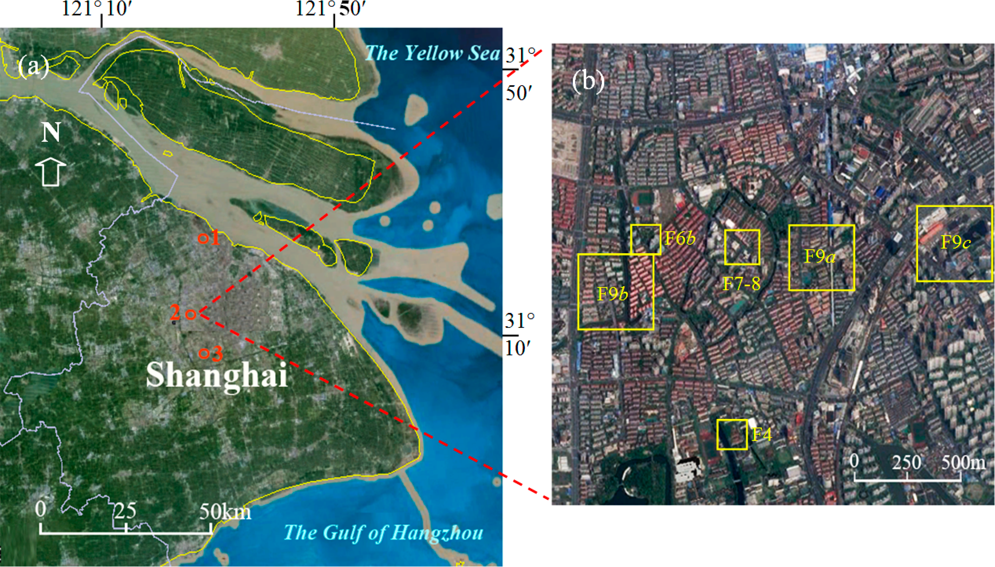
Figure 1 shows the study region.
The test images were randomly selected from nine groups of false-color aerial near-infrared (NIR) images, referred to as “NIR images” in the following text, in a time sequence from 1988 to 2006. The images were purchased from the geographic information service institution of the government. The sensor aboard on was a kind of photogrammetric camera. The original photographic scales were from 1:8000 to 1:15,000 and therefore the spatial resolution at nadir is better than two meters. The original size of photo was 23 cm by 23 cm and they had been assembled into a complete image for each sub- test-region and each date with the geometric and the orthographic corrections before selling. The used film was sensitive to the reflection of NIR band. The photo colors of red, green and blue indicate NIR (760∼850 nm), R (red, 630∼690 nm), and G (green, 520∼600 nm) bands, respectively. In addition, it is a common characteristic of object-based change detection that the detecting accuracy mainly depends on the accuracy of extracting individual object and ignores the spectral similarity between the pairs of images from where the object is extracted. Therefore, the radiation correction of individual image (e.g., atmospheric adjustment) is not as essential as that for the pixel-based change detection.
In Shanghai, likewise with all rainy southern cities in China, NIR images are widely used for city surveying and mapping due to the difficulties in acquiring satellite images all seasons with lower cloud cover. Therefore, it is desirable for them to gain access to the technology of detecting vegetation change from such NIR images.
3. Methods
3.1. Overview
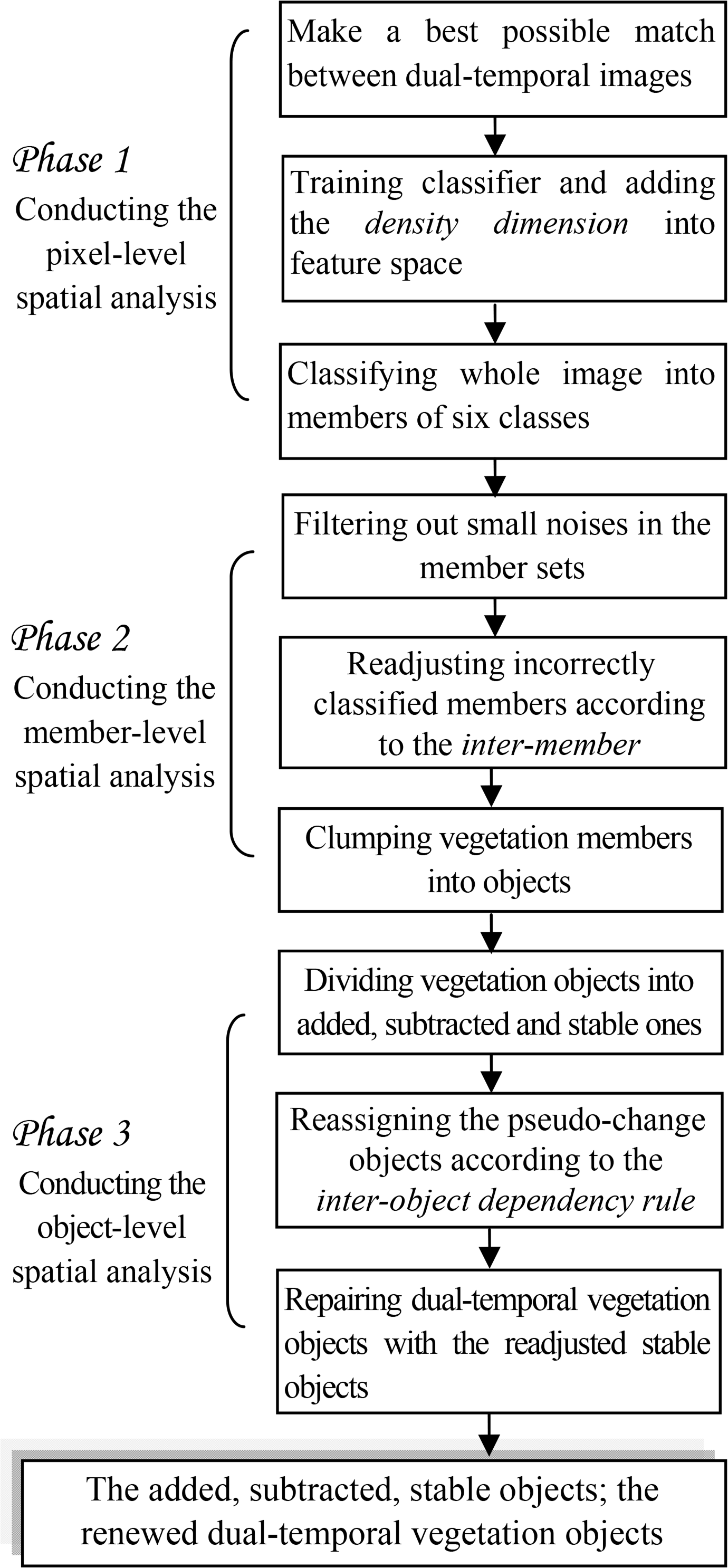
As mentioned previously, the spatial analyses are conducted in three phases. (1) The pixel-level spatial analysis is performed by adding the density dimension to a feature space for classification to indicate the inter-pixel dependency for each pixel; (2) The member-level spatial analysis is conducted by the self-adaptive morphology to readjust the incorrectly classified members according to the inter-member dependency rule; (3) The object-level spatial analysis is realized by the self-adaptive morphology involved with the presetting inter-object dependency rule. The detected spurious changes will be used to repair both dual-temporal vegetation object sets. The added, stable and subtracted objects and the repaired vegetation objects can be finally obtained. Figure 2 shows the flowchart. MATLAB served as the simulation testing tool.
3.2. The Pixel-Level Spatial Analysis
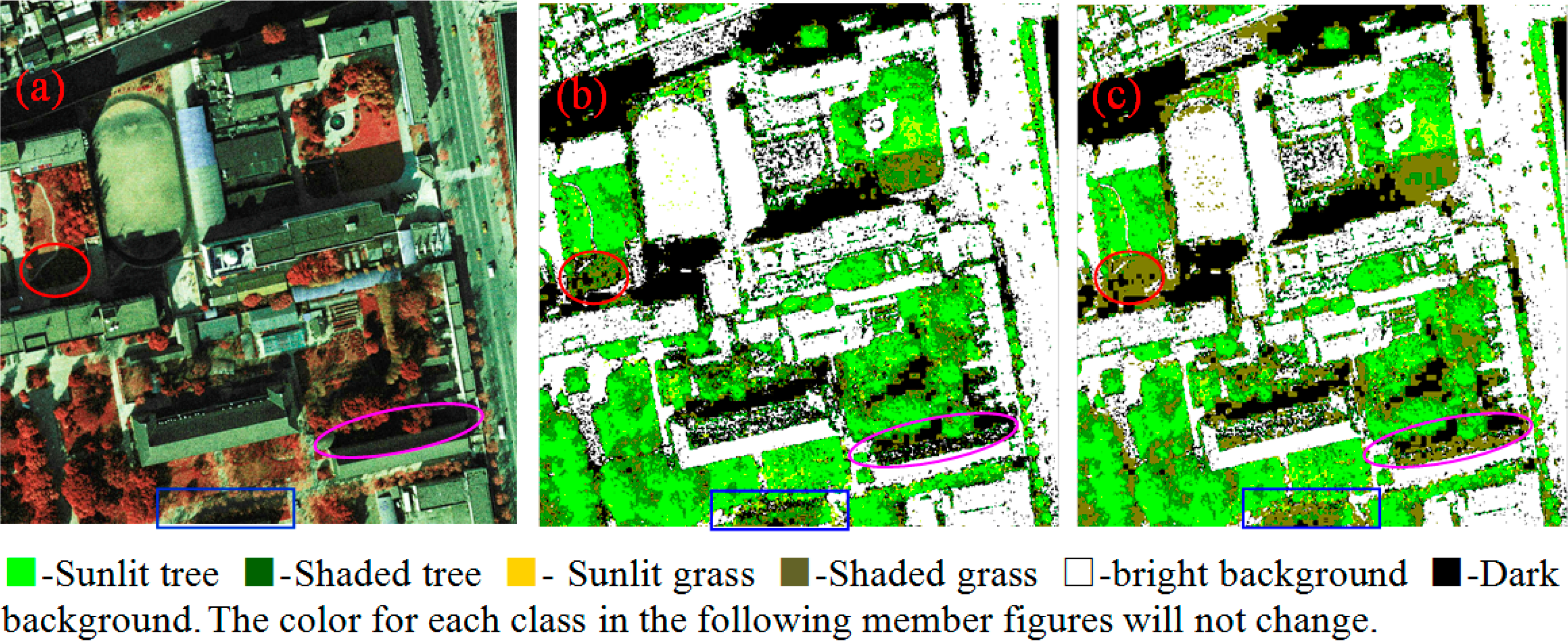
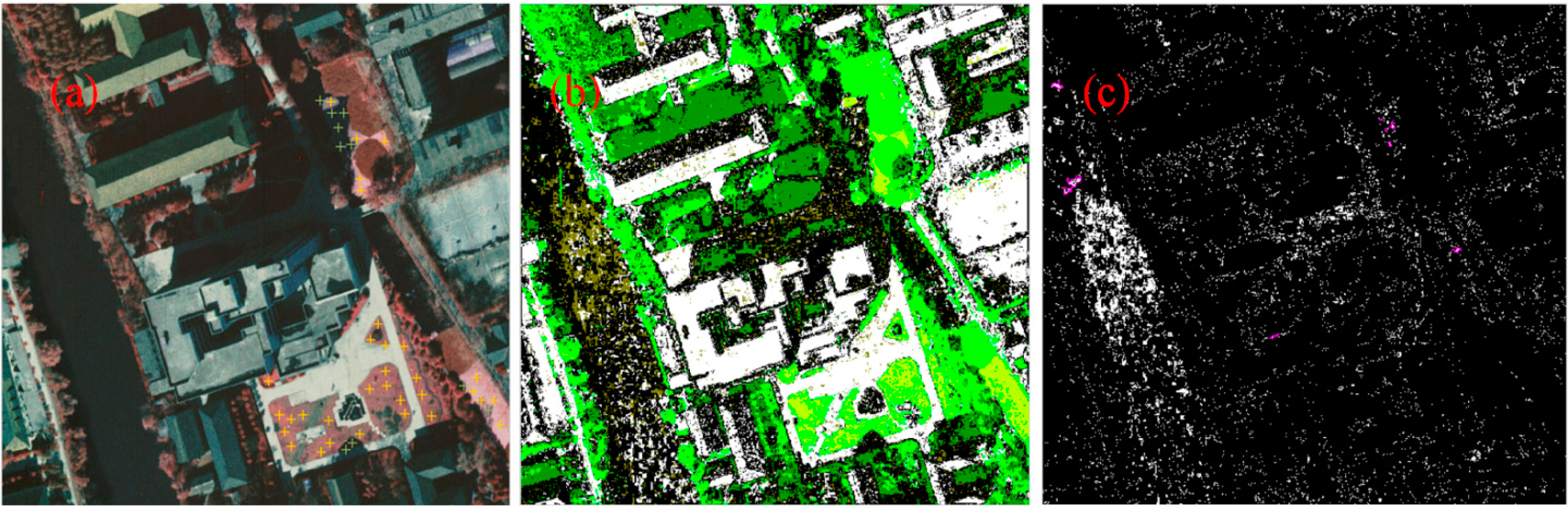
In this phase, the whole image will be classified to the members of different classes through supervised classification. Due to the obvious differences in spectral feature between sunlit and shaded objects and the obvious differences in textural feature between tree and grass on remote sensing imagery of a given resolution, the original six classes include: sunlit tree, shaded tree, sunlit grass, shaded grass, bright background and dark background (involving shaded background and other dark surfaces such as water). Support vector machine (SVM) [26] serves as the model of classifier. In order to make the complexity of the feature space adapt to the number of classes and to highlight the differences in image features between these classes, two spectral and two texture features are utilized (Table 1 [19,27–29]).
Besides the four descriptors, the density dimension, denoted as De, is added to the feature space. De can be understood as a “feature of feature” and is formulated as a density distribution function of multiple features (Equations (1) and (2)). Each element in De represents the density of homogeny neighboring elements. A homogeny element means the pixel with a feature tuple that falls within the tuple of the center element with a given tolerance. With the two equations, the inter-pixel dependency for each pixel can be locally defined in a multi-feature space.
Figure 3 gives an example of the classification with and without De. It can be seen that the identification between different shaded members has been obviously improved by adding De. This may benefit from three novelties: (1) The scale-labeled segments by MRS are replaced with a density field defined by De. The field helps cluster those pixels spatially depart from the patches knitted by other connecting pixels; (2) The homogeneity of pixels is indicated by the density of similar neighboring pixels rather than by SP of MRS. This makes the approach own a better tolerance to image noises; (3) The PS is replaced with dFk. The impact of the accuracy of selecting dFk is far less than that of selecting PS on the classification accuracy. Benefiting from it, a small and relatively stable default of dFk can serve as the tolerance for a single-level segmentation to offer a finer homogeneity between pixels, and the spatial patters created by these homogeneous pixels can be indicated by their density at the same time. Our experiments have revealed that these novelties have great potential for extracting illegible details, such as shaded vegetation members.
3.3. The Member-Level Spatial Analysis
There are four main steps in this phase: (1) removing noises (Section 3.3.1); (2) readjusting misclassified members based on the member-level spatial analysis (Section 3.3.2); (3) knitting vegetation members into objects (Section 3.3.3); and (4) refining objects by interaction (Section 3.3.4).
3.3.1. Removing Noises
Some seriously discrete smaller members should be dealt with as noises before the readjusting to save computational costs because the vegetation members will be individually analyzed afterwards. With the morphological closing, small neighboring members of the same class will be spatially integrated; the rest (those discrete smaller members) will then be removed by area filtering.
3.3.2. Readjusting Misclassified Members Based on the Member-Level Spatial Analysis
After removing the noises, the confusion between shaded grass and dark background members is still commonly apparent, thereby seriously damaging the accuracy of the member. Instead of simply reassigning smaller members by the surrounding majorities as the way of MMUs [5], we use the self-adaptive morphology to depict the inter-member dependency for a more reliable reassigning.
Based on the member-level spatial analysis, each misclassified dark grass member will be readjusted according to the inter-member dependency rule. The dependency for each member can be typically indicated by the density of the neighboring members of involved classes. According to the density, it can be decided whether the center member should be removed as a misclassified or morphologically closed with other involved members. The rule can be formulated as Equation (3).
The self-adaptive morphology is reached by adaptively adjusting t which is the size of the structural element associated with R. The higher the R is, the larger the t will be, and the more the neighboring members will be closed. The algorithm is based on the fact that the higher the R is, the more the members of involved classes around the center member there are and the lower the probability that the central member belongs to noise is. By adjusting t adaptively, the center member can be enlarged to an appropriately integrated vegetation patch. Thus a significant improvement on the accuracy of member can be expected. Figure 4 gives an example.
3.3.3. Knitting Vegetation Members into Objects
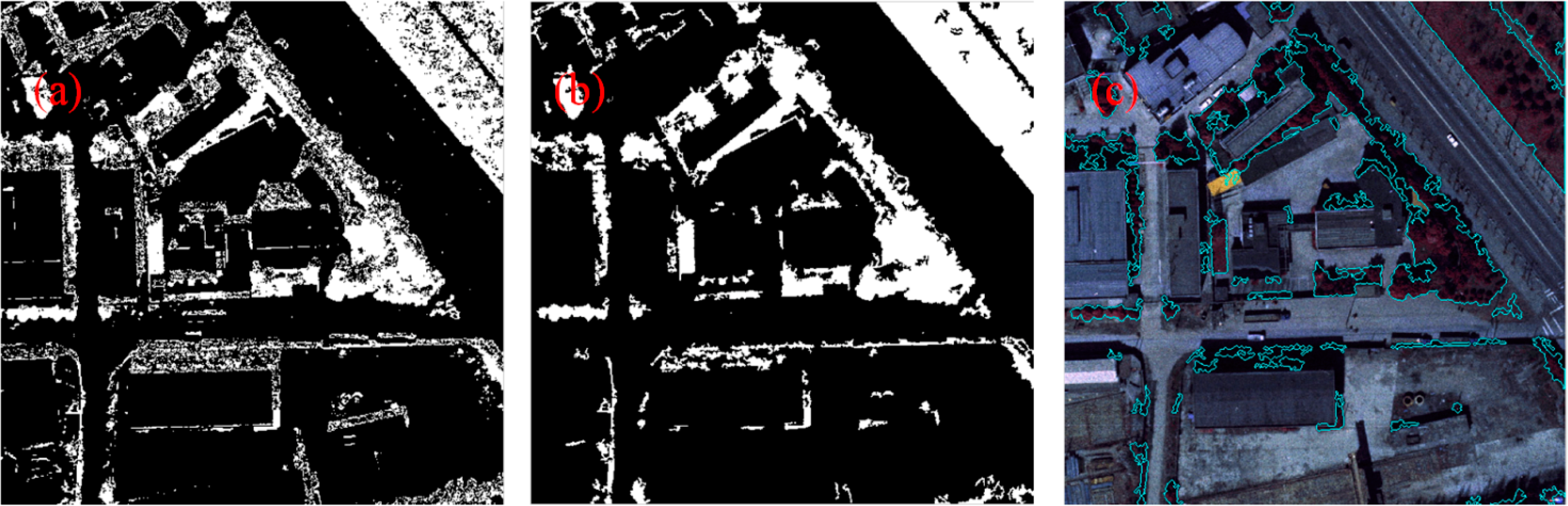
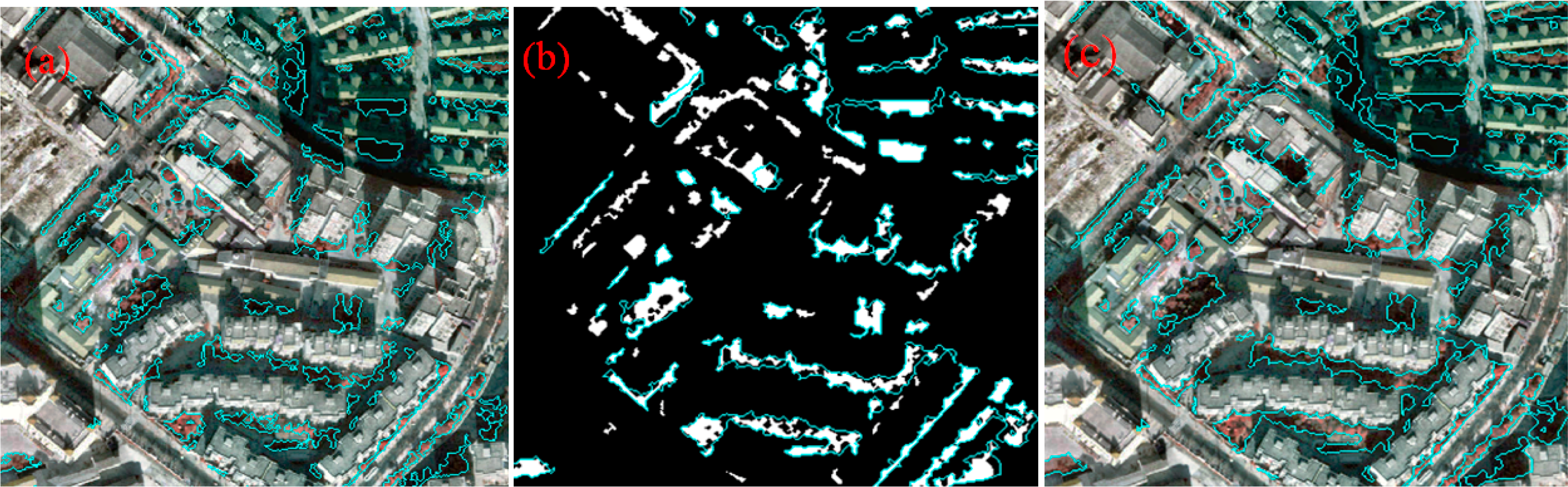
The readjusted members are still scattered and mixed with each other between classes. In general, as long as the members of a class are closely clustered, they can be morphologically knitted to objects, such as bonding discrete members into objects by morphological closing, smoothing object boundaries by morphological opening and removing smaller discrete members by area filtering. Figure 5c gives an example.
In addition, the member-level spatial analysis can also be used to further remove false concaves inside vegetation patches. If a dark background patch is surrounded by a far larger vegetation patch, the former is most likely of a false concave. The area ratio of the former to the latter can serve as a measure for the readjustment. The smaller the ratio is, the higher the probability of the member belonging to a false concave is. Figure 5a,b provide an example.
3.3.4. Refining Vegetation Objects
The originally generated dual-temporal vegetation objects sometimes are insufficiently accurate for change detection and they can be refined by human–computer interaction. There are two new algorithms developed for the refining. One, named as hitting algorithm, is effective in locating the false-present objects and the other, the point expansion algorithm, can be used to generate the false-absent objects.
- (1)
Hitting algorithm
In the following, VS0 is used to denote the binary image of the originally extracted vegetation objects. It is relatively easier to locate the over-extracted patches because they already exist in VS0. By the conventional hitting algorithm, a false-present object can be located when being hit by cursor.
- (2)
Point expansion algorithm
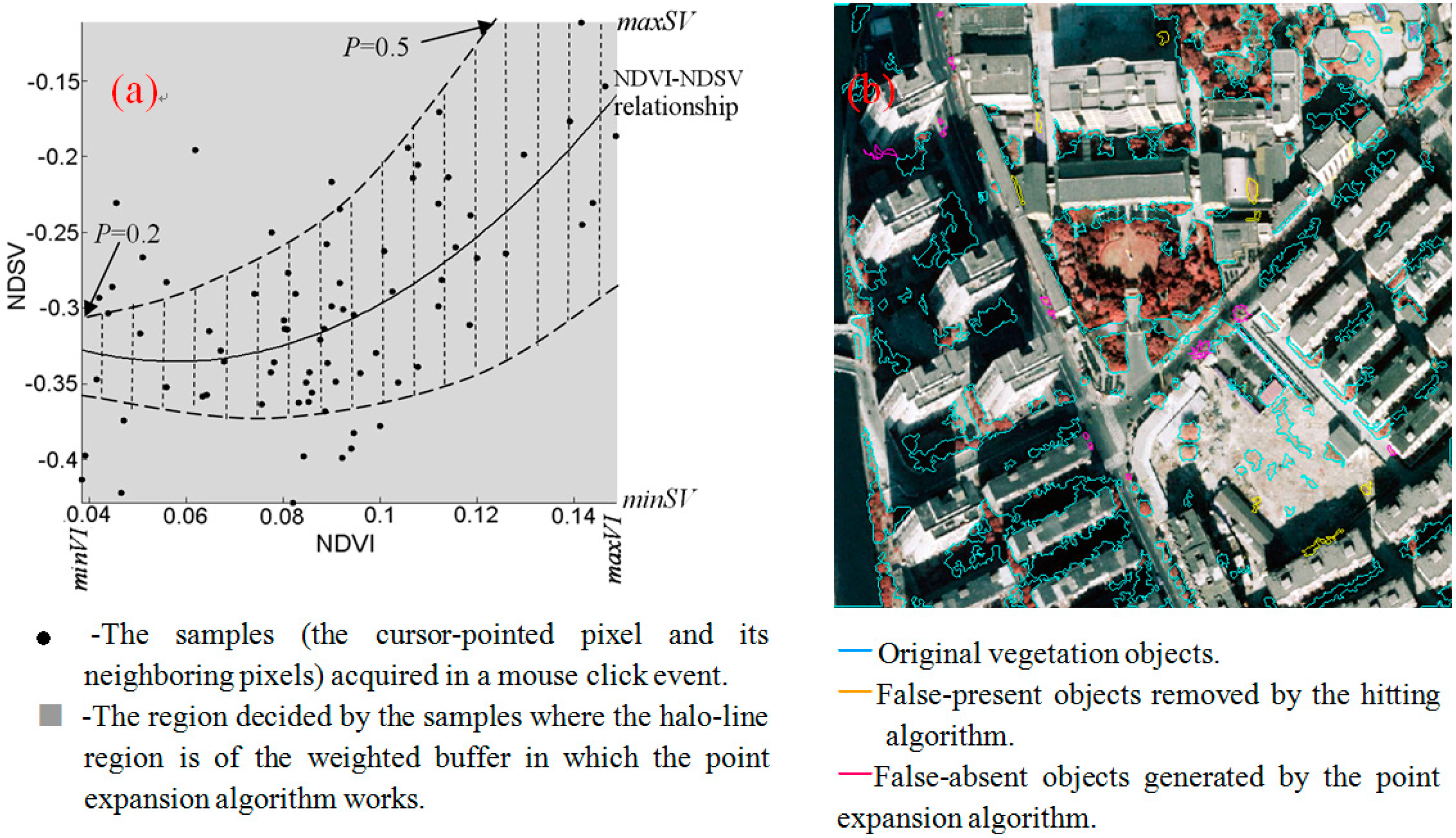
However, to determine a false-absent object is another thing. Its absence from VS0 is resulted from the situation that the majority of pixels in it likely deviate from the mass center of its class in a given feature space. A new algorithm, referred to as the point expansion, has been explored to capture such pixels. Figure 6 gives an example.
Our experiments have revealed that there is a good separability between vegetation and background in the NDVI–NDSV space. Thus the point expansion is conducted through the following steps: (1) taking a cursor-pointed pixel and its neighboring pixels as the samples; (2) deriving a NDVI–NDSV relationship from these samples by a two-order nonlinear fitting; and (3) conducting a seeded region growth within a buffer along the relationship and with these samples as the initial seeds to capture those always under-extracted vegetation pixels. The growing always begins from a more reliable end and searches new vegetation members within the buffer. The weights will make the width of the buffer gradually narrowed as the separability worsens. The growing process can be formulated as Equation (4).
In order to avoid the unexpected entrance of smooth dark background members, a during-growing constraint, termed the “expansion rate,” is proposed (Equation (5)).
ER is usually stable during the iteration but increases suddenly when a larger body of dark smooth background (e.g., water and shaded roads) enters the iteratively expanding region. Therefore, Condition (c) of Equation (4) serves as a constraint on ER to limit the unexpected entrance. T2 is of a threshold with an experimental default of 3. It is possible to achieve the best separation between shaded vegetation and smoother dark background by adjusting T2. Figure 6 provides an example. Additionally, the hitting algorithm and point expansion can also serve as a tool for the late accuracy assessment (Section 4.1).
3.4. The Object-Level Spatial Analysis
There are three main steps in this phase: (1) detecting spurious changes through use of the object-level spatial analysis and then revising both of the dynamic and stable object sets (Section 3.4.1); (2) recovering the misjudgments by interaction (Section 3.4.2); and (3) repairing the original dual-temporal vegetation object sets by merging the renewed stable into both of them (Section 3.4.3).
3.4.1. Detecting Spurious Changes
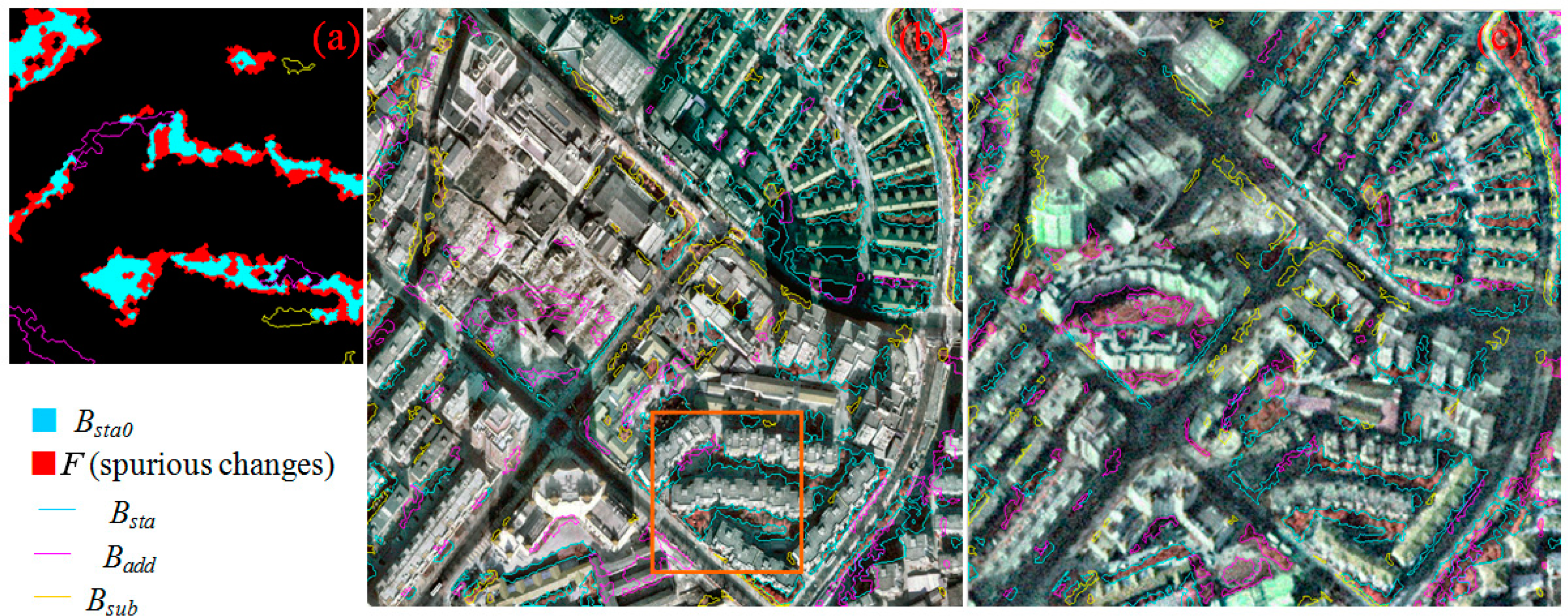
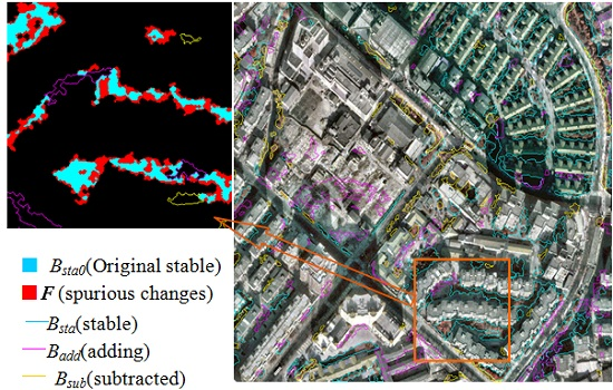
Before the detection, the dual-temporal vegetation objects are divided into three sets: the added, the subtracted and the stable (Badd0, Bsub0 and Bsta0) which denote the new, the disappearing and the stable objects respectively through use of per-pixel binary logical operations. There usually are considerable spurious changes in the initial dynamic object sets (Badd0 and Bsub0) due to variations in sun angle and sensor look angle. The accuracy of the stable objects will also be seriously damaged. The efforts mentioned before to improve the accuracy of the member can merely reduce the area of a pseudo-change patch and make it easier to be detected in this step.
The dependency rule for the object-level spatial analysis is potentially available by assessing how closely a dynamic object is located to a stable one. For example, a dynamic object will be most likely of a part of a stable one if the area of the former is far less than that of the latter and they have long shared boundaries at the same time. Assessed by such an inter-object dependency rule, most spurious changes can be detected. The rule can be formulated as Equation (6).
The rule can be linguistically described as: (1) when a dynamic object is located at an end of a stable one, the area of the former is smaller than T3 and the intersection of the dilated former and the latter is not empty; (2) when a dynamic object is near a side of a stable one, the two objects have length-sufficient shared boundaries and the area of the former is smaller. If any of the two conditions is satisfied, the former will be added to F. Then all the objects in F will be merged into Bsta0 and will also be removed from their original sets at the same time. Figure 7 gives an example of this process. Bsta, Badd and Bsub represent the renewed sets from Bsta0, Badd0 and Bsub0, respectively. It is revealed by the accuracy assessment that more than 97% of spurious-change objects can be detected.
3.4.2. Recovering Misjudgments by Human–Computer Interaction
Another version of the hitting algorithm for recovering the misjudgments has been explored. Some recovering operations will be executed in accordance with the properties of mouse click events. Either a hit dynamic object will be reassigned to Bsta or the hit part from a stable object will be recovered for its original dynamic status. If the differences between before and after the revisions are referred to as errors, the new version of the hitting algorithm can also serve as a tool to assess the accuracy of vegetation change detection.
3.4.3. Repairing Dual-Temporal Vegetation Objects
It is not rare that a vegetation object is less shaded by buildings or with no building shelter in one of the image pairs due to variations in sun angle and sensor look angle. The objects in F usually indicate the variations. Therefore, taking these objects as supplements, the shaded and the obscured vegetation objects can be repaired afterwards. Figure 8 provides an example.
4. Results and Discussion
In this section, the accuracy of extracting vegetation object and detecting spurious change will be assessed separately.
Both the extraction and detection address only binary splitting. The former divides pixels into vegetation and background and the latter divides the vegetation objects into dynamic and stable ones. Instead of using the confusion matrix which is fit for assessing the accuracy of classification between multiple classes, we use the relative errors to indicate the splitting mistakes. In addition, the incorrect vegetation objects, including under and over extracted ones, and the incorrect changes, including false stable and false dynamic ones, cannot become aware before the vegetation objects being extracted and the changes being detected. In most cases, such objects may not be collected as the reserved checking-samples for accuracy assessment in the sampling phase since they usually do not have the typical appearances of their respective classes. Therefore, they were practically collected as accurately as possible by human–computer interaction with the hitting and the point expansion algorithms to guarantee an objective assessment.
4.1. The Accuracy of Extracting Vegetation Object
Four scenes (Figure 3 and Figure 6) are for the accuracy assessment and Table 2 provides the results. Different combinations of spatial analyses are tested in each example to ensure both the spatial analyses at the levels of pixel and members. The feature space, the model of classifier and the original classes are the same as those of the example in Section 3.2.
As mentioned previously, the false-absent and false-present patches in the original object set can be located and then repaired by human–computer interaction. The differences between before and after the repair are referred to as errors for the accuracy assessment (Table 2). It can be seen that the accuracy of automatic extraction of vegetation objects with both the pixel and the member-level spatial analyses is pretty good and only few of them need to be recovered by the interaction. The errors are no more than 2.56%, 7.04% and 12.15% for the cases of with both the pixel and the member-level spatial analyses, with only the pixel-level spatial analysis and with no spatial analysis respectively.
4.2. The Accuracy of Detecting Vegetation Changes
The accuracy assessment is carried out through use of the hitting algorithm mentioned in Section 3.4.2. The differences between before and after the repair are referred to as errors. Four pairs of images provided in Figures 7 and 9 are for the assessment and Table 3 provides the results. The assessment follows the first three steps of the object-level spatial analysis given in the beginning of Section 3.4.
The data in Table 3 reveal that the accuracy of detecting spurious changes through use of the object-level spatial analysis is also so good that only a few of objects are misjudged by computer. The objects need to be recovered by human–computer interaction is only 2.03% on average and no more than 3.26% out of all the dynamic objects in area. The interactive recovery is likely required to deal with the off-nadir issues when vegetation locates close to higher buildings (e.g., the object pointed by red arrow in Figure 9c1).
5. Conclusions
This paper presents a novel method to improve change detection accuracy of the urban vegetation using high-resolution remote sensing images. The following conclusions can be supported by the aforementioned work. (1) The proposed approach takes advantage of series of spatial analyses at multi-levels which can help to significantly reduce the error of the extracted objects and the detected spurious changes; (2) All the spatial analyses in different levels connect one after another and each of them has been proved to be indispensable in the entire process. The errors from the automatic extraction of vegetation objects are no more than 2.56%, 7.04% and 12.15% for the cases with both pixel and member-level spatial analyses, with only pixel-level spatial analysis, and with no spatial analysis, respectively. The error from the automatic detection of spurious changes with the object-level spatial analysis is no more than 3.26%. It means that only no higher than 2.56% of incorrectly extracted vegetation objects and 3.26% of misjudged dynamic objects need to be recovered by human–computer interaction; (3) The limitation of the approach is mainly caused by the dependence on the position matching of two date images; otherwise the error from the detected spurious changes would increase heavily. However, the accurate position matching in a dense high-rise building area is difficult to reach because parts of the reference points in the ground for the matching are often sheltered by buildings. Thus, a method with better tolerance to this shortcoming is appreciated.
Acknowledgments
We would like to express our gratitude to Brian Finlayson, University of Melbourne, Australia and Professor Minhe Ji, East China Normal University, China, for their reviews and many helpful suggestions. The work presented in this paper is supported by the National Natural Science Foundation of China (Grant No. 41071275).
Author Contributions
Jun Qin analyzed the data. Jianhua Zhou performed the experiments and wrote the paper. Bailang Yu revised the paper.
Conflicts of Interest
The authors declare no conflict of interest.
References
- Coppin, P.; Jonckheere, I.; Nackaerts, K.; Muys, B. Digital change detection methods in ecosystem monitoring: A review. Int. J. Remote Sens 2004, 25, 1565–1596. [Google Scholar]
- Small, C.; Lu, W.T. Estimation and vicarious validation of urban vegetation abundance by spectral mixture analysis. Remote Sens. Environ 2006, 100, 441–456. [Google Scholar]
- Berberoglu, S.; Akin, A. Assessing different remote sensing techniques to detect land use/cover changes in the eastern Mediterranean. Int. J. Appl. Earth Obs. Geoinf 2009, 11, 46–53. [Google Scholar]
- Coops, N.C.; Wulder, M.A.; White, J.C. Identifying and describing forest disturbance and spatial pattern: Data selection issues and methodoloical implications. In Understanding Forest Disturbance and Spatial pattern: Remote Sensing and GIS Approaches; Wulder, M.A., Franklin, S.E., Eds.; CRC Press: Boca Raton, FL, USA, 2006; pp. 33–60. [Google Scholar]
- Colditz, R.R.; Acosta-Velázquez, J.; Díaz Gallegos, J.R.; Vázquez Lule, A.D.; Rodríguez-Zúñiga, M.T.; Maeda, P.; Cruz López, M.I.; Ressl, R. Potential effects in multi-resolution post-classification change detection. Int. J. Remote Sens 2012, 33, 6426–6445. [Google Scholar]
- Chan, J.C.; Chan, K.; Yeh, A.G. Detecting the nature of change in an urban environment: A comparison of machine learning algorithms. Photogram. Eng. Remote Sens 2001, 67, 213–225. [Google Scholar]
- Rafiee, R.A.; Salman, M.A.; Khorasani, N. Assessment of changes in urban green spaces of Mashad city using satellite data. Int. J. Appl. Earth Obs. Geoinf 2009, 11, 431–438. [Google Scholar]
- Prakash, A.; Gupta, R.P. Land-use mapping and change detection in a coal mining area—A case study in the Jharia Coalfield, India. Int. J. Remote Sens 1998, 19, 391–410. [Google Scholar]
- Bindschadler, R.A; Scambos, T.A.; Choi, H.; Haran, T.M. Ice sheet change detection by satellite image defferencing. Remote Sens. Environ 2010, 114, 1353–1362. [Google Scholar]
- Coppin, P.R.; Bauer, M.E. Digital change detection in forest ecosystems with remote sensing imagery. Remote Sens. Rev 1996, 13, 207–234. [Google Scholar]
- Malila, W.A. Change vector analysis: An approach for detecting forest changes with Landsat. Proceedings of the Machine Processing of Remotely Sensed Data Symposium, West Lafayette, IN, USA, 3–6 June 1980; pp. 326–335.
- Wulder, M.A.; Ortlepp, S.M.; White, J.C.; Coops, N.C. Impact of sun-surface-sensor geometry upon multitemporal high spatial resolution satellite imagery. Can. J. Remote Sens 2008, 34, 455–461. [Google Scholar]
- Chen, G.; Hay, G.J.; Carvalho, L.M.T.; Wulder, M.A. Object-based change detection. Int. J. Remote Sens 2012, 33, 4434–4457. [Google Scholar]
- Small, C. Estimation of urban vegetation abundance by spectral mixture analysis. Int. J. Remote Sens 2001, 22, 1305–1334. [Google Scholar]
- Pu, R.L.; Gong, P.; Michishita, R; Sasagawa, T. Spectral mixture analysis for mapping abundance of urban surface components from the Terra/ASTER data. Remote Sens. Environ 2007, 112, 939–954. [Google Scholar]
- Van der Linden, S.; Hostert, P. The influence of urban structures on impervious surface maps from airborne hyperspectral data. Remote Sens.Environ 2009, 113, 2298–2305. [Google Scholar]
- Prati, A.; Mikic, I.; Trivedi, M.M.; Cucchiara, R. Detecting moving shadows: Algorithms and evaluations. IEEE Trans. Pattern Anal. Mach. Intell 2003, 25, 918–923. [Google Scholar]
- Tsai, V.J.D. A comparative study on shadow compensation of color aerial images in invariant color models. IEEE Trans. Geosci. Remote Sens 2006, 44, 1661–1671. [Google Scholar]
- Zhou, J.H.; Zhou, Y.F.; Guo, X.H.; Ren, Z. Methods of extracting distribution information of plants at urban darken areas and repairing their brightness. J. E. China Norm. Univ. (Natl. Sci. Ed.) 2011, 6, 1–9. [Google Scholar]
- Gao, X.J.; Wan, Y.C.; Zheng, S.Y.; Li, J. Automatic shadow detection and compensation of aerial remote sensing images. Geomat. Inf. Sci. Wuhan Univ 2012, 37, 1299–1302. [Google Scholar]
- Hofmann, P.; Blaschke, T.; Strobl, J. Quantifying the robustness of fuzzy rule sets in object based image analysis. Int. J. Remote Sens 2011, 32, 7359–7381. [Google Scholar]
- Blaschke, T.; Hay, G.J.; Kelly, M.; Lang, S.; Hofmann, P.; Addink, E.; Feitosa, R.; van der Meer, F.; van der Werff, H.; van Coillie, F.; et al. Geographic object-based image analysis: A new paradigm in remote sensing and geographic information science. ISPRS Int. J. Photogram. Remote Sens 2014, 87, 180–191. [Google Scholar]
- Blaschke, T. Object based image analysis for remote sensing. ISPRS Int. J. Photogram. Remote Sens 2010, 65, 2–16. [Google Scholar]
- Baatz, M.; Schäpe, A. Multiresolution segmentation—An optimization approach for high quality multi-scale image segmentation. In Angewandte Geographische Informationsverarbeitung XII; Strobl, J., Blaschke, T., Griesebner, G., Eds.; Wichmann-Verlag: Heidelberg, Germany, 2000; pp. 12–23. [Google Scholar]
- Drăguţ, L.; Csillik, O.; Eisank, C.; Tiede, D. Automated parameterisation for multi-scale image segmentation on multiple layers. ISPRS Int. J. Photogram. Remote Sens 2014, 88, 119–127. [Google Scholar]
- Bennett, K.P.; Campbell, C. Support vector machines: Hype or Hallelujah? SIGKDD Explor 2000, 2, 1–13. [Google Scholar]
- Price, J.C. Estimating vegetation amount from visible and near infrared reflectances. Remote Sens. Environ 1992, 41, 29–34. [Google Scholar]
- Zhou, J.H.; Zhou, Y.F.; Mu, W.S. Mathematic descriptors for identifying plant species: A case study on urban landscape vegetation. J. Remote Sens 2011, 15, 524–538. [Google Scholar]
- Huete, A.R. A soil-adjusted vegetation index (SAVI). Remote Sens. Environ 1988, 25, 295–309. [Google Scholar]


| Sign | Name | Meaning | Applicability |
|---|---|---|---|
| NDVI | Normalized Difference Vegetation Index [27] | NDVI = (IR − R)/(IR + R) where IR and R are the DNs of NIR and red bands, respectively. | Distinguishing between vegetation and background. |
| NDSV | Normalized Difference of Saturation and Brightness [19] | NDSV = (S − V)/(S + V) where S and V are saturation and brightness in the Hue- saturation-brightness color system. | Distinguishing between shaded vegetation and dark background |
| Cd | Density of low-NIR pixels | Cd = Sp/A [a] where Sp is a supplemental pixel set. Sp = {BWlow∩!BWhigh, BWlow|NDVI > a × TNDVI & SAVI > 1.5 × a × TNDVI, BWhigh|NDVI > TNDVI}[b,c] | Extracting winter deciduous tree crowns. |
| Dd | Density of dark details [28] | Dd(k) = COUNT(BWd(k))/Aplant(k) [a,d] BWd = {BWd ⊆ I, BWd|(I•se−I)>c×d where BWd(k) is the kth block of a binary image of dark detail; d is the mean size of dark detail; I is a gray image; • and se, the sign of morphological closing and its structure element; c is a coefficient. | Dd is sensitive to the variations of crown roughness. Different Dd matrices involved with d can often server as independent features in a feature space (e.g., the example in Figure 3). |
[a]A = Block area; Aplant = vegetation-covered area in a block.[b]BWhigh and BWlow = Binary images of vegetation cover associated with normal and lowered thresholds respectively. SAVI = Soil-adjusted vegetation index [29]. The condition of SAVI > 1.5 a·TNDVI can often work well for BWlow to extract low-NIR reflection crowns where a is of a coefficient with the experimental defaults of 0.6 in summer and 0.3 in winter, respectively.[c]TNDVI = The threshold for the segmentation of NDVI with a widely used experimental default of 0.17 for extracting vegetation from NIR images.[d]COUNT(•) = Counting function for the number of true members in a binary image.
| Figure No. | AVS (pixels) | Error with no Spatial Analysis (%) | Error with the Pixel-Level Spatial Analysis only (%) | Error with Both the Pixel and Member-Level Spatial Analyses (%) | ||||||
|---|---|---|---|---|---|---|---|---|---|---|
| Eunder | Eover | Etotal | Eunder | Eover | Etotal | Eunder | Eover | Etotal | ||
| 4 | 335,340 | 2.66 | 5.48 | 8.14 | 0.86 | 4.44 | 5.30 | 0.47 | 0.51 | 0.98 |
| 5 | 195,250 | 1.63 | 7.04 | 8.67 | 0.87 | 6.17 | 7.04 | 0.85 | 1.71 | 2.56 |
| 6 | 108,640 | 2.98 | 9.17 | 12.15 | 2.33 | 1.74 | 4.08 | 1.34 | 0.5 | 1.84 |
| 3 | 191,510 | 1.26 | 9.57 | 10.83 | 0.77 | 1.58 | 2.34 | 0.46 | 0.81 | 1.27 |
| Mean | 2.13 | 7.81 | 9.95 | 1.21 | 3.48 | 4.69 | 0.78 | 0.88 | 1.66 | |
| Maximum | 2.98 | 9.57 | 12.15 | 2.33 | 6.17 | 7.04 | 1.34 | 1.71 | 2.56 | |
| Figure No | Year | Image size | Adyn0 (pixels) | Adyn (pixels) | Ddyn (%) |
|---|---|---|---|---|---|
| 7 | 2000/2003 | 1020 × 1125 | 80,756 | 83,392 | 3.264779 |
| 9a | 1993/2003 | 441 × 496 | 47,245 | 48,393 | 2.43081 |
| 9b | 2000/2005 | 512 × 496 | 29,681 | 29,538 | −0.48345 |
| 9c | 2003/2006 | 893 × 954 | 67,890 | 66,566 | −1.94967 |
Davg = 2.03%; Dmax = 3.26%
© 2014 by the authors; licensee MDPI, Basel, Switzerland This article is an open access article distributed under the terms and conditions of the Creative Commons Attribution license (http://creativecommons.org/licenses/by/3.0/).
Share and Cite
Zhou, J.; Yu, B.; Qin, J. Multi-Level Spatial Analysis for Change Detection of Urban Vegetation at Individual Tree Scale. Remote Sens. 2014, 6, 9086-9103. https://doi.org/10.3390/rs6099086
Zhou J, Yu B, Qin J. Multi-Level Spatial Analysis for Change Detection of Urban Vegetation at Individual Tree Scale. Remote Sensing. 2014; 6(9):9086-9103. https://doi.org/10.3390/rs6099086
Chicago/Turabian StyleZhou, Jianhua, Bailang Yu, and Jun Qin. 2014. "Multi-Level Spatial Analysis for Change Detection of Urban Vegetation at Individual Tree Scale" Remote Sensing 6, no. 9: 9086-9103. https://doi.org/10.3390/rs6099086
APA StyleZhou, J., Yu, B., & Qin, J. (2014). Multi-Level Spatial Analysis for Change Detection of Urban Vegetation at Individual Tree Scale. Remote Sensing, 6(9), 9086-9103. https://doi.org/10.3390/rs6099086