Monitoring Depth of Shallow Atmospheric Boundary Layer to Complement LiDAR Measurements Affected by Partial Overlap

Abstract
: There is compelling evidence that the incomplete laser beam receiver field-of-view overlap (i.e., partial overlap) of ground-based vertically-pointing aerosol LiDAR restricts the observational range for detecting aerosol layer boundaries to a certain height above the LiDAR. This height varies from one to few hundreds of meters, depending on the transceiver geometry. The range, or height of full overlap, is defined as the minimum distance at which the laser beam is completely imaged onto the detector through the field stop in the receiver optics. Thus, the LiDAR signal below the height of full overlap remains erroneous. In effect, it is not possible to derive the atmospheric boundary layer (ABL) top (zi) below the height of full overlap using lidar measurements alone. This problem makes determination of the nocturnal zi almost impossible, as the nocturnal zi is often lower than the minimum possible retrieved height due to incomplete overlap of lidar. Detailed studies of the nocturnal boundary layer or of variability of low zi would require changes in the LiDAR configuration such that a complete transceiver overlap could be achieved at a much lower height. Otherwise, improvements in the system configuration or deployment (e.g., scanning LiDAR) are needed. However, these improvements are challenging due to the instrument configuration and the need for Raman channel signal, eye-safe laser transmitter for scanning deployment, etc. This paper presents a brief review of some of the challenges and opportunities in overcoming the partial overlap of the LiDAR transceiver to determine zi below the height of full-overlap using complementary approaches to derive low zi. A comprehensive discussion focusing on four different techniques is presented. These are based on the combined (1) ceilometer and LiDAR; (2) tower-based trace gas (e.g., CO2) concentration profiles and LiDAR measurements; (3) 222Rn budget approach and LiDAR-derived results; and (4) encroachment model and LiDAR observations.
1. Introduction
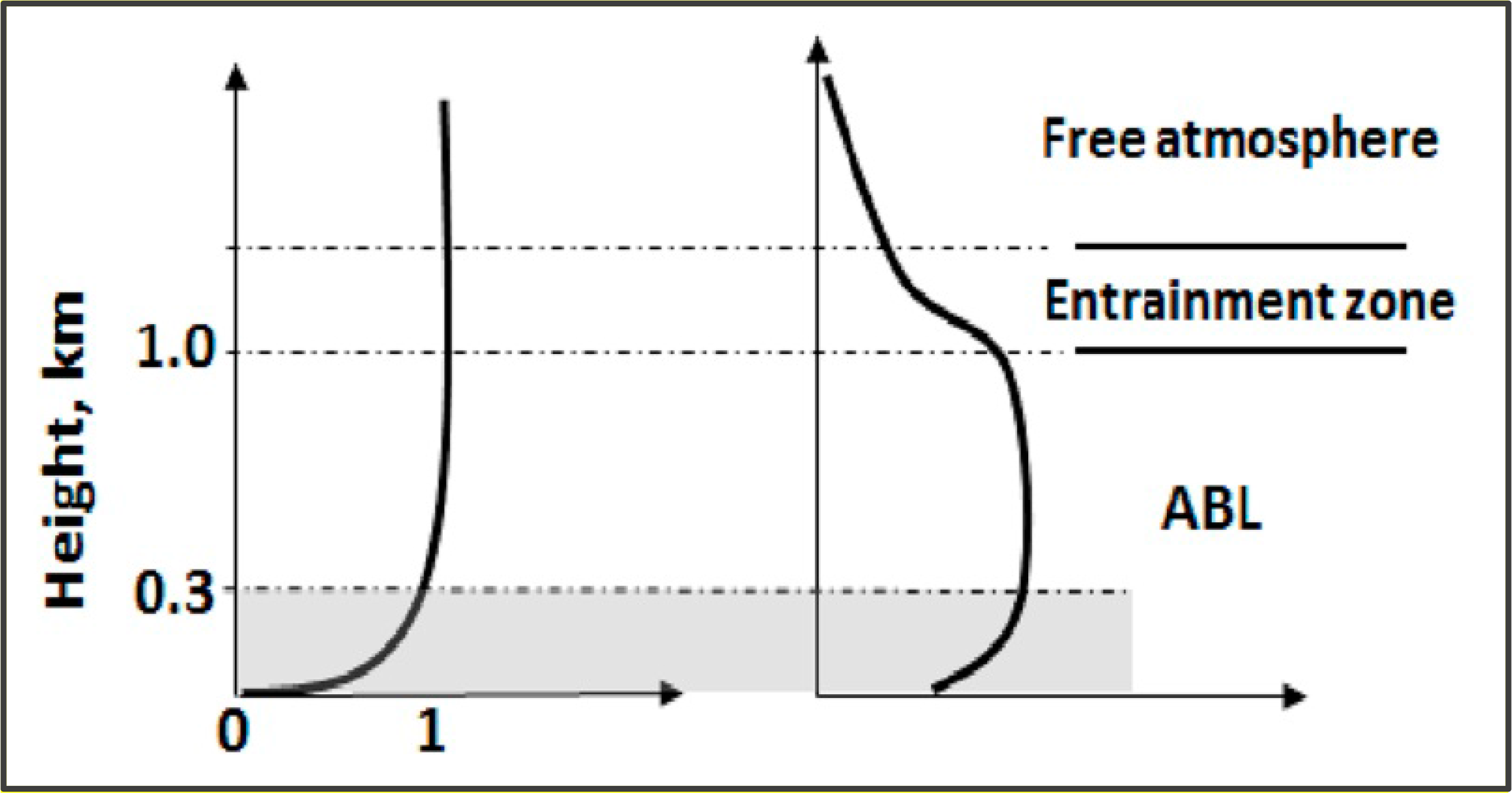
The atmospheric boundary layer (ABL) and the entrainment zone primarily govern the mixing of pollutants into the upper troposphere, which influences air quality and climate simulation [1]. The depth of the ABL and the growth rate of the ABL in the morning are important parameters for characterizing many atmospheric processes, including land-atmosphere exchange processes and the dispersion of air pollutants and the formation of clouds [2–4]. Ground-based remote sensing techniques (e.g., LiDAR, ceilometer) are useful tools for monitoring ABL depths [5–7]. The potential of high vertically and temporally resolved aerosol backscatter measurements with LiDAR and ceilometer offers an excellent opportunity to determine the top of the ABL (zi). In the last three decades different methods have been developed to determine zi from ground-based LiDAR and ceilometer measurements, [7–14] and from the space-borne LiDAR system CALIPSO [15–17]. In particular, numerous studies have been performed to determine daytime convective boundary layer (CBL) topped by the clean, free atmosphere (FA). These studies used different techniques, namely threshold detection (e.g., [18]), the gradient-based method (e.g., [19]), the inflection point method (e.g., [20]), the variance analysis (e.g., [21]), the Haar wavelet approach (e.g., [14]), the combined wavelet and image processing method [22], the ideal profile method (e.g., [23]), and the 2-D gradient approach [24] to derive zi using aerosol LiDAR measurements.
LiDAR systems are used to monitor daytime zi since: (1) aerosols are good tracers of turbulent mixing; (2) there are over 30 years of studies on aerosol backscatter gradients and variances; (3) there is temporal coverage in the daytime ABL regime; and (4) there is spatial coverage with networks of LiDARs/ceilometers around the world (e.g., [22,24]). However, the development of a zi retrieval algorithm that is both automated and applicable at all times and under different meteorological conditions still remains a challenge (e.g., [13,21]). Since the aerosols may exist in multiple stratifications the correct attribution of the layer at the top of the mixing layer is not trivial, and deriving retrieval uncertainties from LiDAR profiles alone certainly remains another challenge [8,13]. Numerous efforts were made to resolve this issue of attribution (e.g., [21,25]). For instance, the SIRTA (Site Instrumental de Recherche par Télédétection Atmosphérique) observatory conducted studies based on long-term time series of collocated profiling measurements, and found that the use of ancillary data makes the aerosol-based estimations of ABL depth more physically reliable under a wide spectrum of conditions (e.g., [20,21]). Numerous reviews have also been carried out in the past to address this attribution issue (e.g., [8–10]). However, some limitations of LiDAR systems include the LiDAR transceiver overlap effect, aerosol washout due to rain, and presence of light attenuating water clouds with high optical depth (e.g., [20,21,24–27])]. In particular, zi-dynamics and associated aerosol stratification cannot be well understood due to the incomplete knowledge of the LiDAR response at all ranges which is posed by the partial overlap function (i.e., the geometrical form factor or crossover function) [5,6]. This issue yields a systematic effect. Thus, the application of ground-based LiDAR systems is useful for the situation of a deep, convective ABL; however, for stable atmospheric conditions often observed at night when the ABL is too shallow (i.e., zi lies below the height of full overlap), LiDAR measurements need to be supplemented with other techniques to finally determine the entire diurnal cycle of zi.
The height of the full overlap defines the distance (often called the “dead-zone”) from the LiDAR to the first detectable and useful aerosol backscatter signal in the entire profile. Due to the LiDAR transceiver overlap effect, determination of depth of shallow CBL, and often nocturnal boundary layer (NBL), remain almost impossible using only LiDAR measurements. In fact, the LiDAR overlap makes the zi undetectable below this limit. In case of a very low zi, which frequently occurs under stable conditions at night and sometimes during the day, particularly in winter, this offset can actually mask the early growth of CBL height and can also lead to erroneous results in monitoring shallow ABL in the daytime. This issue has been given little attention in the literature as far as LiDAR-determination of ABL depth is concerned (e.g., [21,25,26]).
In this article, some of the potential approaches that could overcome the partial overlap effect of LiDAR systems to monitor shallow ABL are first discussed. A brief review is then presented on the opportunities and the challenges of overcoming the partial overlap effect using complementary measurements with some recommendations for near future research. The key aim of the different sections of this review is to identify and discuss some of the critical issues in monitoring shallow ABL, and in particular to help the scientific community address NBL depth variability in detail. Within the ongoing scientific projects related to the boundary layer process studies at the SIRTA observatory, it has been clearly recognized that improvement in the zi retrieval algorithms by determining the zi lying below the full-overlap is an important step to improve numerical models dedicated to the boundary layer process studies in both regional [28–31] and global scales (e.g., [32]). In general, this is an important aspect for routine monitoring of zi using aerosol LiDAR measurements. Additionally, there is a strong need of more robust zi retrieval algorithm, associated with retrieval uncertainties and reliability flags (e.g., [24,31]).
The remaining part of the article is organized as follows. Section 2 briefly summarizes the importance of monitoring shallow ABL. Some of the experimental and theoretical methods that allows for retrieving the overlap function and correct LiDAR-derived signal for further processing are discussed in Section 3. Four different approaches to derive the entire diurnal cycle of zi are addressed in Section 4; both potential and limitation of these methods are discussed. Finally, Section 5 provides a brief summary and draws conclusions.
2. Importance of Monitoring Shallow Atmospheric Boundary Layer
The concentrations of passive trace gases within the ABL do not vary only because of changes in the mixing volume (i.e., ABL depth), but they also change due to boundary layer dynamics associated with the growth rate of zi, which determines the entrainment of FA air into the ABL (e.g., [1,2]). The FA air entrained into the ABL has different thermodynamic and chemical properties; in particular, the concentrations of the tracers like radon, CO2, water vapor, CO, CH4, N2O, aerosol particles, drop significantly from ABL to the FA, as was found by many researchers in the past (e.g., [33,34]).
Therefore, it cannot be excluded that the tracer concentrations within the ABL, are affected by the growth rate of the zi in the morning, in addition to the zi itself via ABL dilution effect, or so-called “volume effect”. In fact, the ABL depth acts as a “first-order” control for the vertical extent of the “box” within which mixing and dispersion of the tracers like GHGs (CO2, CH4, N2O, etc.), aerosol particles, ozone, and 222Rn, etc. take place [35–38]. Characterization of the temporal variability of zi during entire diurnal cycle is therefore required. For instance, the ecosystem CO2 exchange and the ABL mixing are correlated diurnally and seasonally via the “rectifier effect,” which has been thoroughly documented (e.g., [39]). Thus, the assessment of the effect of carbon sequestration and/or greenhouse gas emissions reduction activities, including attribution of sources and sinks by region and sector is a challenging but important task [38–41]. In estimating the CBL growth rate during the early morning transition or in studying dispersion in a shallow CBL [42–44], determination of zi below the height of full overlap of a LiDAR system is urgently required. Additionally, a growing CBL during the morning transition period first interacts with the overlying residual layer (RL) and then with the FA after reaching the quasi-stationary height. Both these interactions have an impact on the growth rate, and consequently on the mixing processes and relevant dilution of the tracers in the boundary layer [39,45]. Therefore, determination of the depth of shallow NBL/shallow CBL/growing CBL over the land surface is considered important for dispersion studies and for monitoring air quality.
3. Theoretical and Experimental Approaches to Correct LiDAR Signal for Overlap Factor
In the simplest form, the LiDAR-received signal intensity can be expressed as [4]
Most of today’s automated and test-bed research lidars around the world are not capable of determining low ABL depths (∼100–200 m). To obtain a comprehensive overview on the partial overlap of the LiDAR transceiver system, a few important factors need to be discussed first. It is also important to understand the geometric reasons for the systematic error causing difficulties in monitoring shallow ABL, in particular, NBL. Figure 1 shows a schematic of a simple mono-static bi-axial aerosol LiDAR system illustrating the effect of partial overlap on the LiDAR measurements. In principle, the overlap function O(R) describes the competency in performance of a LiDAR with which light is coupled into its detectors as a function of range (i.e., height as we describe here vertically-pointing LiDAR system). In Equation (1), the value of O(R) is zero at the LiDAR and becomes 1 when the volume of space containing the transmitted pulse is completely imaged onto the detector through the field stop [46]. Thus, from the top of the LiDAR transceiver to the height of full overlap (where O(R) = 1), O(R) varies in height with values from 0 to 1 (Figure 1). This is referred to as partial overlap region.
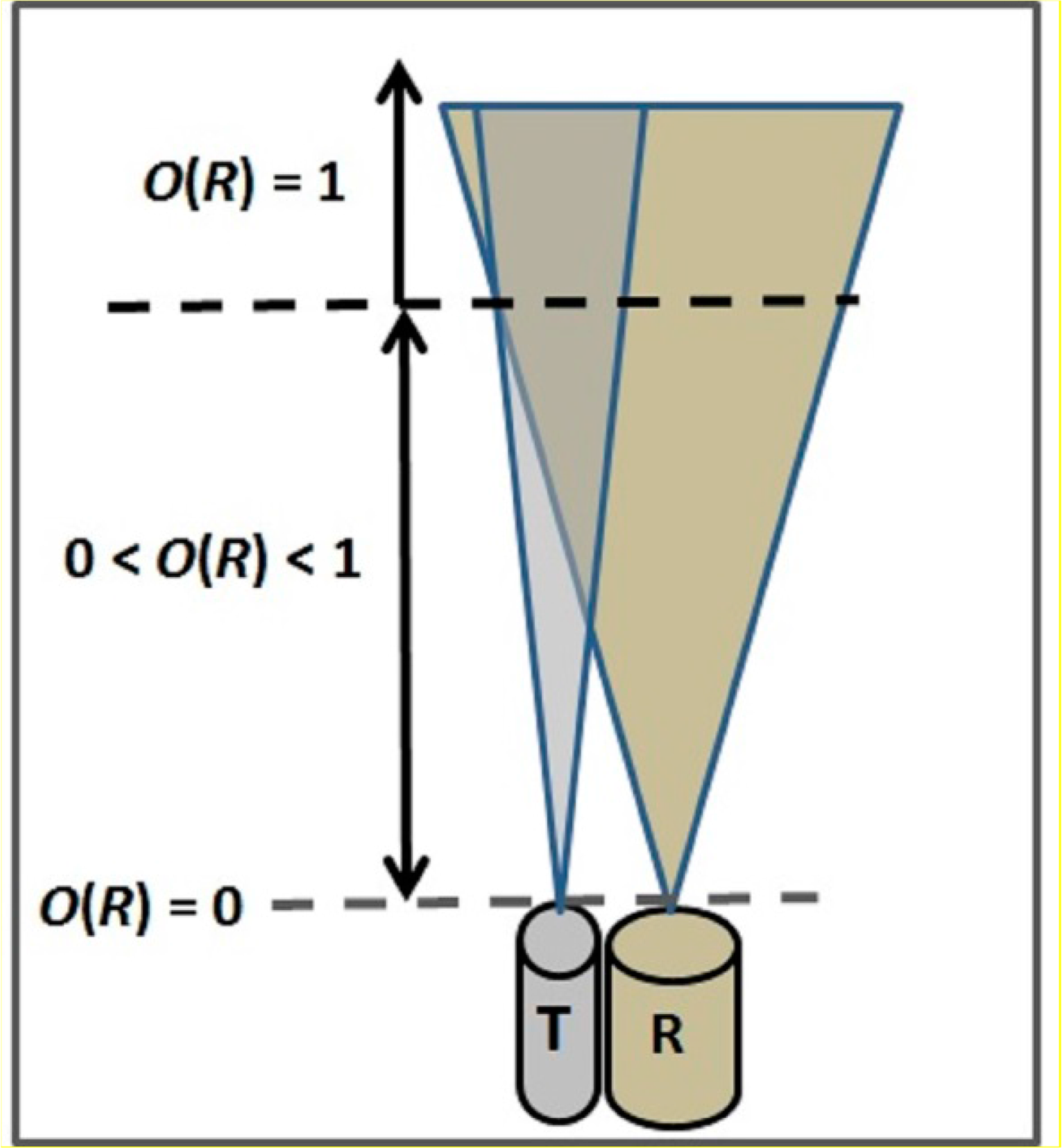
The height dependence of O(R) is further illustrated in Figure 2. By tuning an iris placed in the focal plane of the telescope, the receiving telescope’s field of view can be increased so that the overlap range can be reduced and the height of full overlap becomes lower. However, it should be noted that there is a compromise between the incomplete overlap and the background light noise which need to be maintained to achieve a better signal-to-noise ratio (SNR). In general, the overlap function mainly depends on the geometry of the LiDAR transceiver setup. For instance, co-axial LiDAR systems with the transmitter and receiver having the same optical axes are also affected by the partial overlap effect due to misalignment in the receiver optics (e.g., [46,47]). On the other hand, in many LiDAR systems with large telescopes (more than 50-cm diameter) full overlap (i.e., O(R) of 1) is achieved at a distance of more than 1 km (e.g., [47,48]). For LiDAR systems with a smaller telescope (between 20 and 40 cm diameter), the complete overlap is found to be between 150 and 600 m above ground (e.g., [46–50]). Significant errors exist in the profile of the LiDAR signal received from the region of incomplete overlap, i.e., close to the ground where the aerosol particles are both most abundant and most variable [49]. Consequently, the partial overlap introduces a systematic error in the LiDAR measurements because it precludes the determination of the depth of the shallow and stable ABL (especially at night). If the LiDAR signals are corrected for partial overlap (i.e., O(R) becomes unity and independent of height), an objective routine to determine zi is available and a robust attribution is applied, the diurnal cycle of zi could be achieved using a LiDAR system only. However, there are challenges with this method, as will be discussed in the following pages.
Figure 2 exemplifies a profile of range-dependent O(R), explaining that the full-overlap of the transceiver is attained at about 300 m distance. Determination of the zi below 300 m would thus require changes in the LiDAR configuration to obtain a complete transceiver overlap at a much lower range. Although the real structure in the ABL, entrainment zone and zi is more complex than shown, this figure still provides a useful information for relating O(R) to LiDAR backscatter profile. Wandinger and Ansmann [51] introduced an experimental approach to determine O(R), which requires a pure molecular backscatter channel (Raman signal) in addition to the usual elastic backscatter signal. This method works well for the 355 and the 532 nm channels using Raman signals under both homogeneous and inhomogeneous conditions without any critical assumption, unlike some theoretical approaches (e.g., slope method, polynomial regression, non-linear regression) illustrated by Tomine et al. [52], Dho et al. [53], Povey et al. [54], among others. However, Guerrero-Rascado et al. [55] found poor performance of Raman-signal approach for 1064 nm-channel of a LiDAR system due to the low intensity for the Raman shifted signal in the infrared range.
On the other hand, to compensate the differences in the overlap functions resulting from the wavelength-dependent beam divergence, Markowicz et al. [56] proposed a multi-axial design for their multi-wavelength LiDAR system where each of the laser beams is emitted separately and the respective position between the beam and telescope’s axes can be adjusted. Recently, Biavati et al. [57] proposed an experimental technique to estimate an overlap correction function. They introduced an iterative procedure to retrieve an experimental correction and a fitting procedure to obtain a modeled correction which yielded promising results. However, this correction factor could be achieved only if the LiDAR system could be oriented at angles different than 90°. On the other hand, measurements obtained by operational LiDARs like micro-pulse LiDAR (MPL) deployed within NASA’s MPL-NET are also affected by the partial overlap and need additional measurements of horizontal profiles up to a ∼10 km clear line-of-sight and homogenous atmospheric conditions which is often challenging to achieve due to the inhomogeneity of aerosol structures within the ABL (e.g., [58]). Berkoff et al. [59] developed an experimental approach for correcting the partial overlap of the MPL using a secondary receiver that eliminates the need for horizontal measurements. However, their technique requires a specific configuration of additional optical components (detector, filters, data channel, etc.) and co-alignment of receivers.
Another approach to obtain near-range signal below the height of complete overlap is by improving the entire LiDAR transceiver geometry by adding a smaller telescope. For instance, Behrendt et al. [35] demonstrated two receiving telescopes for a state-of-the-art water vapor DIAL system: an 80-cm telescope in vertically-pointing mode for the far field and a 20-cm telescope for the near field. Additionally, they also found an improvement in the overlap factor by introducing a fiber-based transmitter for the high-power laser in their LiDAR system. The water vapor DIAL system developed by Behrendt et al. [47] is a unique system but due to its complexity this type of LiDAR system requires high expenditure, significant amount of maintenance, advanced and high power laser technology, etc. Thus, we suggest that this system or any other two-telescope bi-axial LiDAR system is not a suitable candidate for operational monitoring of zi though it is an excellent instrument for field deployments (e.g., [48]). On the other hand, numerous custom-made vertically-pointing aerosol LiDAR systems are operational around the world within different networks like ICOS, GALION, etc. (e.g., [24,31]); further improvement in their optical geometry or modifications of any other instrumental feature is not straightforward.
Additionally, by pointing a laser beam in various directions at various angles (scanning) with respect to the surface, a ground-based aerosol LiDAR system can provide a description of the three-dimensional distribution of aerosols in the atmosphere [60–63]. Range height indicator (RHI) scanning measurements can help obtain low zi starting from a distance where complete overlap is reached [56]. The RHI scanning measurements were used only within some feasibility studies and/or case studies using data obtained during field campaigns. Notwithstanding, all range eye-safety in the transmitted laser beam needs to be maintained for these LiDAR systems (e.g., [62,63]), otherwise they cannot be deployed in urbanized areas. Additionally, scanning LiDAR systems usually require high-power laser transmitters to achieve useful SNR in the off-zenith profiles due to the trade-off in range/height relationships with scanner elevation angles in the RHI mode (e.g., [47]).
Deployment of nadir-pointing airborne LiDAR systems does not pose any challenges for monitoring shallow ABL as long as an appropriate mission plan is made by flying the aircraft well-above the zi [64–66]. Airborne LiDAR measurements do not make low zi retrieval erroneous since the overlap-affected part of the LiDAR signal remains in the FA atop a CBL. However, contamination due to ground-returns makes the LiDAR signals erroneous close to ground so that few bins (corresponding to 100 m or more depending on the range resolution) close to the ground create saturation in the detectors (e.g., [66]). In any case, operational monitoring of zi with airborne LiDAR measurements is not regarded a practical approach.
In summary, it is possible to overcome the problem of the partial overlap via improving LiDAR system configuration, using two-telescope receiver configuration, by changing the deployment or platform of the LiDAR instrument, or via some experimental/theoretical approaches by calculating an overlap correction function or other method based on Raman channel. Additionally, using common optics for both transmitter and receiver (mono-static configuration) or by imaging the laser beam side with a wide-angle camera, it is possible to overcome the effect of partial overlap factor (e.g., [67,68]). However, these solutions often become technically challenging, highly expensive, and unrealistic as soon as operational monitoring of zi is concerned. They are also limited due to the inhomogeneous aerosol structures often present in the ABL. For instance, we are not familiar with any scanning LiDAR system that is operational for routine monitoring of zi. While using a mono-static LiDAR, Eresmaa et al. [69] found that low ABL depth was not determined well. Under these circumstances, an alternative method needs to be sought or additional information would be beneficial to incorporate into the retrieval algorithms so that the shallow ABL could also be monitored on regular basis with vertically-pointing single-channel elastic LiDAR systems. Recently, some researchers showed potential for using near-surface meteorological and micrometeorological parameters in the zi retrieval algorithm to help the attribution (e.g., [21,25,70]), however, problems related to the partial overlap factor are yet to be solved. In the following, a comprehensive overview on four different approaches to complement LiDAR-derived time series of zi is presented.
4. Supplementary Methods to Determine the Depth of Shallow Atmospheric Boundary Layer
4.1. Ceilometer and LiDAR Measurements
Ceilometers use similar principles as in LiDAR systems. In general, a ceilometer transmits fast, low-powered laser pulses into the atmosphere and detects the back-scattered returns from clouds and aerosols above the instrument. Ceilometers are mostly dedicated to cloud base height/cloud layer measurements and vertical visibility for meteorological and aviation applications. However, due to recent progresses in low-cost laser systems, ceilometers have been found useful for detecting aerosols in general and especially for detecting volcanic ash layers, and recently for determining zi (e.g., [50]). Many researchers in the past discussed in detail the potential differences between the efficiency of LiDAR and ceilometer systems for monitoring ABL (e.g., [24]). Due to the low power of the laser transmitter used in the ceilometer, the performance of the ceilometer with respect to SNR is much better in the nighttime than it is during the day, when aerosol particles are generally concentrated enough to provide a strong gradient in the NBL [24]. In contrast, the high SNR of LiDAR signals even for daytime measurements yields the advantage to monitor the CBL height without ambiguity. For instance, while comparing the performance of a Jenoptik ceilometer, Hesse et al. [71] found a considerable increase in the SNR and dynamic range (by a factor of 2) for NBL compared to daytime CBL. Additionally, while comparing performance of LiDAR and ceilometer, Tsaknakis et al. [72] found that during the daytime the CL31 ceilometer was able to correctly detect the presence of various aerosol layers only after averaging the signals for sufficiently longer term period (3 h). An averaging time of more than few tens of minutes is not suitable for determining CBL depths, in particular during the morning transition period, when CBL depth often increases with a growth rate of more than 300 m/h (e.g., [45,50]).
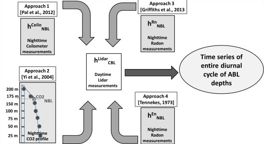
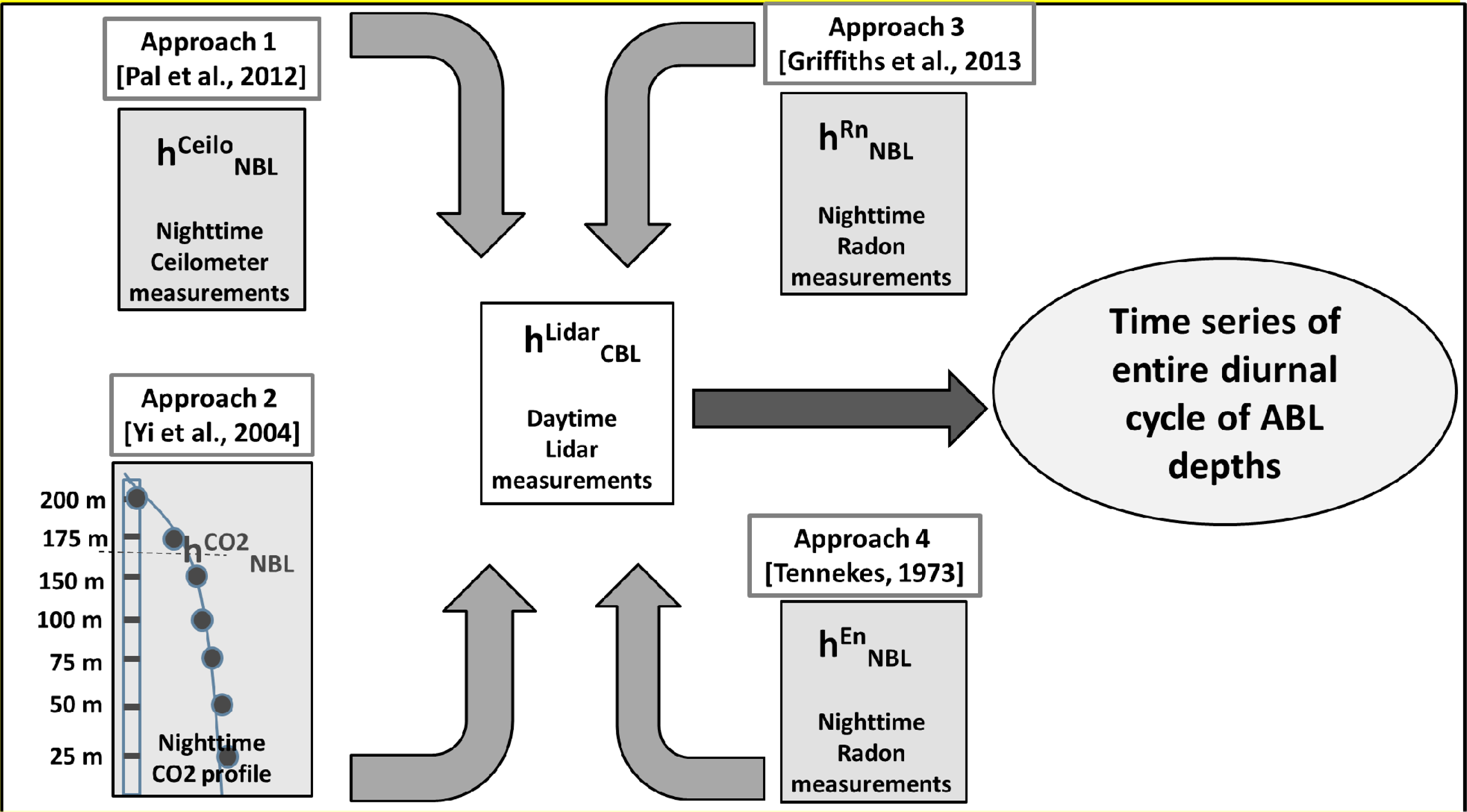
The most remarkable differences between LiDAR and ceilometer systems lie in their overlap factor and the power of the laser transmitter used. Most of the today’s ceilometers use an enhanced single-lens technology in their transceiver and thus have excellent performance starting at the first bin, corresponding to 15–30 m [73–75]. Therefore, these systems do not suffer from the partial overlap factor that vertically-pointing LiDAR systems do, and have system efficiency over the entire measuring range (with respect to the overlap issue). This efficiency helps obtain significantly improved near-range performance for monitoring shallow NBL. Thus, ceilometers are found to be important candidates, in particular for monitoring the transition from stable boundary layer (SBL) to CBL, or from shallow CBL to a growing CBL regime [50]. On the other hand, due to the high power laser transmitter used in the LiDAR systems, they are suitable for monitoring daytime CBL height with sufficient accuracy as was demonstrated by many researchers in the past. Pal et al., [50] while investigating zi variability around Paris, used concurrent measurements obtained with both LiDAR and ceilometer systems. Finally, they used combined zi measurements: a ceilometer was used for the NBL and LiDAR was used for the daytime CBL. Figure 3 presents a schematic for obtaining entire diurnal cycle of zi using combined LiDAR and ceilometer based approaches.
It should be noted that both LiDAR and ceilometer systems use aerosols as tracers to determine the zi. The only drawback in this approach is that simultaneous LiDAR and ceilometer measurements at a site would be required. However, during field campaigns or routine measurements at different observatories around the world like SIRTA, ACRF (ARM Climate Research Facility), CIAO (CNR-IMAA Atmospheric Observatory), CESAR Observatory (Cabauw), among others, both instruments are usually available (e.g., [31,76]). Thus, we suggest that if an appropriate attribution technique is chosen [21,24], LiDAR-ceilometer retrieval results in a correct estimate of zi; an uncertainty of around 15–30 m exists due to sampling of aerosol signal at different heights depending on range resolutions in the data.
4.2. Tower-Based Trace Gas Concentration Profile and LiDAR Measurements
The depth of the ABL plays an important role in controlling the concentration of GHGs and other tracers like aerosols due to the ABL dilution effect, often referred to as vertical mixing term in a mass budget (e.g., [2,39]). There is compelling evidence that ABL dilutes the surface CO2 flux during both night and day as well as during different seasons in a year (e.g., [77–79]). In general and on a daily basis, during the nighttime, RL CO2 is sampled at the upper part of a tall tower on flat terrains, while at the lower levels a relatively higher concentration of CO2 is observed (Figure 3). In the present context, we refer to towers with heights of around 100 m or more for monitoring GHGs and meteorological variables as tall towers (e.g., [78–82]). The CO2 concentrations at lower levels are affected by nocturnal accumulation, creating a gradient at the upper level of the tower [79]. The diurnal variability of the CO2 mixing ratio on flat, homogeneous terrain is mainly determined by the surface CO2 flux, CO2 advection, and the volume of air in which the CO2 is mixed. It thus depends on the depths of the ABL both during day and night. The NBL depth can be derived from vertical profiles of the CO2 mixing ratio since CO2 is an excellent indicator of stratification. Yi et al. [83] determined the entire diurnal cycle of zi by combining the measurements from 915-MHz boundary layer profiling radar and CO2 concentrations obtained at six levels on a 447-m tall tower. They used a tower-based CO2 profile to determine both the SBL depths in the night and the low CBL depths during morning. Following Yi et al. [80], they defined the top of the SBL at which CO2 gradients first become very small. Finally, they complemented these measurements with the profiler measurements. The working principle of zi retrieval using wind profilers lies in the determination of the location of the peak reflectivity caused by turbulence acting on a gradient of humidity at zi ([27]). In Yi et al. [83], the profiler measurements were not able to define ABL shallower than 400 m. Under similar assumptions, Denning et al. [81] derived the entire diurnal cycle of zi by combining radar reflectivity and vertical profiles of CO2 made on a tall tower in northern Wisconsin.
Recently, Schmidt et al. [79] illustrated that during the nighttime the vertical profiles of CO2 mole fraction at the four sampling heights on the 180-m tall Trainou tower usually exhibited strong gradients within the NBL, while Pal et al. [50] found that the aerosol LiDAR at the same site was not able to accurately detect the boundary layer aerosol structures and associated mixing processes taking place in the NBL due to the partial overlap effect. Following the previous studies illustrating the combination of radar/wind profiler and tower-based CO2 profile measurements, we suggest that by combining LiDAR and tower-based CO2 profiles one can also monitor the entire diurnal cycle of ABL depths: LiDAR for daytime CBL depths and tower-based CO2 profiles for NBL depths. Hence, the issues related to the partial overlap could be resolved. It should be noted, however, that the NBL depths derived with the CO2 profile-based approach would be based on coarse resolution (30 to 50 m or higher depending on the sampling heights) unlike high-resolution LiDAR measurements (15 m or lower). Thus, some sort of interpolation would be required in the CO2 profiles and should be carefully handled before this gradient-based approach is applied. Some sensitivity tests are highly recommended for the choice of the interpolation scheme as was performed in Yi et al. [83]. One should note that applications of the CO2-profile based approach will most likely fail to determine NBL depths over mountainous regions, and in particular at ridge-top sites since orographically-induced flow (e.g., upslope flow) will often affect the patterns of the diurnal cycle of CO2 or any other tracers in these regions [84,85].
It should be noted here that while exploring six years of trace gas measurements on 180 m tall tower in Trainou (France), Schmidt et al. [79] found that tracers other than CO2 like methane (CH4), sulfur hexafluoride (SF6), molecular hydrogen (H2), nitrous oxide (N2O), and carbon monoxide (CO) show nocturnal gradient similar to those found for CO2. Therefore, we consider that when using the gradient-based approach, tower-based profiles of these tracers could be also used for routine monitoring of NBL depths over flat terrain. The main drawback of the proposed approach is that the installation of tall towers are more expensive than simply acquiring a ceilometer, since towers hundreds of meters tall always require considerably more maintenance. However, for the experimental sites within different networks (e.g., ICOS, AmeriFlux, NOAA tall tower network, etc.) where tall-tower measurements already exist, the trace gas profile-based approach could be applied as a parallel approach to determine low ABL depths to complement LiDAR measurements that are affected by partial overlap effect. An uncertainty of around 50 m in the zi arises if an appropriate gradient is not chosen during the sensitivity analyses of choosing the correct inflection point.
4.3. 222Rn tracer method and LiDAR-Derived Results
The naturally occurring, radioactive noble gas radon (222Rn) is an ideal passive tracer for investigating atmospheric transport and mixing processes within the ABL (e.g., [86]). 222Rn is an inert gas emanating from soils and rocks containing 226Ra. Since its half-life (3.83 days) is much longer than the timescales of turbulence in a CBL (<1 h), it is considered as a conservative tracer for mixing in the ABL; it is also a useful timescale for determining rates of soil-atmosphere gas exchange [87–90]. Additionally, its half-life is sufficiently short to ensure that typical concentrations in the FA are orders of magnitude lower than within the ABL. Williams et al. [91] while investigating vertical profiles of 222Rn, found a marked drop in concentrations from high values within the ABL (typically around 4 ± 3 Bq·m−3) to near-zero values in the FA (around 0.5 ± 0.4 Bq·m−3). We consider that due to the simplicity of the processes affecting radon concentration in the ABL (e.g., half-life of 3.83 d, contrasts in ABL-FA, radioactive decay as the only sink, etc.), with a few assumptions it is straightforward to derive zi from a time series of 222Rn concentrations for NBL regime (i.e., from time of sunset to the time when CBL starts developing after next day’s sunrise).
Assuming horizontal homogeneity, the time series of 222Rn concentrations can be inverted to determine an effective mixing height (e.g., [92]). This method is appropriate for NBL regimes (Figure 3). Duenas and Fernandez [93] illustrated that temporal variability in the 222Rn concentration due to changes in the exhalations rate is of second order compared to vertical turbulent mixing mechanism, except in very prolonged periods of heavy precipitation, or when the surface is covered by snow or ice. A mass balance approach illustrates that in a non-divergent flow field and in the absence of horizontal advection of 222Rn, the temporal variation in the 222Rn mean concentration in the CBL, is driven by the sum of the surface emissions, radioactive decay, and vertical mixing (dilution) within the ABL (e.g., [39,92]). The corresponding relationship can be expressed as:
Using radon-based zi estimations, numerous researchers estimated trace gas fluxes (e.g., N2O) during nocturnal inversions or SBL regimes or synoptic events (e.g., [94–96]). In addition, following a similar approach, Griffiths et al. [92] derived an improved mixing height retrieval algorithm where the key focus was to improve the attribution technique when LiDAR signals encounter multiple aerosol layers. This technique can be used for shallower SBL or for the periods when the zi measurements are affected due to the partial overlap effect. Thus, this technique could potentially complement LiDAR measurements below the full-overlap height if a reliable attribution technique is applied for the LiDAR measurements collected over the height of full-overlap during the daytime [13,34,50]. However, during the morning transition period with slow growth of CBL, the radon-based tracer method would not be applicable for obtaining low zi below the height of full overlap. However, for the CBL regime with rapid growth rate (say 200–300 m/h), zi quickly reaches beyond the height of full overlap so that LiDAR becomes useful.
It should be noted that the application of the radon-based approach requires the knowledge of the rate of emission of radon gas from the soil and information about the footprint of the radon concentrations measured at a site, which are site-specific. In general, radon flux F in Equation (6) is directly measured with flux chambers at various sites where tower-based radon measurements are available. There is ongoing effort to estimate radon flux using maps of soil composition, soil uranium content and soil moisture ([97]). Additionally, when advection dominates the measurements and soils are covered with snow or ice, the radon-based approach is not considered to be a very useful approach (e.g., [92]). An uncertainty of around 30–50 m arises if the measurements of radon flux are not available and theoretical estimations are used.
4.4. Encroachment Model and LiDAR-Derived Results
Near-surface thermodynamics and micrometeorological features during the morning transition period play an important role in governing the development of the CBL throughout the morning until the time when the CBL height reaches a quasi-stationary regime (e.g., [98,99]). Following an encroachment model introduced by Tennekes [98], a simple hypothesis has been developed to detect only the low CBL top rising from below the full overlap height during the early morning transition period. According to this assumption, the zi starts growing immediately after crossover (when the heat flux changes sign from negative to positive) followed by sunrise.
Following the encroachment model introduced by Tennekes [98], one can relate the changes in the ABL depths during morning transition period as:
Using LiDAR -measured zi above the height of full-overlap one can determine z2 using any of the gradient-based techniques discussed above. To determine z1, one can use Equation (7) going backwards in time until the time of crossover (dt = T2 − T1 with T2 > T1) [21]. Using this method one cannot determine the NBL depths for the entire nighttime period. However, determination of growth rate of ABL is possible with this approach. As explained previously, this determination is very important in studying the dilution of pollutants and other tracers in the atmosphere during the morning transition period. Using this approach, one can also determine dzi/dt experimentally using LiDAR-measured zi after the height of full overlap. Finally, a comparison could be done with dzi/dt for the period before the time when zi reaches the full-overlap. Corresponding results will definitely help understand in detail the transition from SBL (or NBL) to CBL (or shallow CBL) during the morning transition period. It should be mentioned that this method would work for the LiDAR measurements on days when well-mixed CBL development takes place, likely during fair weather, anti-cyclonic conditions without the presence of optically thick clouds in the boundary layer and large scale subsidence (e.g., [1,50]).
5. Summary and Conclusions
Ground-based single-channel aerosol LiDAR systems have attracted much attention in recent decades. The availability of automated and robust aerosol LiDAR systems around the world have made LiDAR remote sensing of boundary layer processes more versatile than ever before. Routine monitoring of the entire diurnal cycle of atmospheric boundary layer depths is an important but a challenging task. Within numerous research projects and networks around the world (e.g., EU COST Action ES0702, EG-CLIMET, ARM, ICOS, GALION, MPL-NET, etc.) ground-based vertically-pointing aerosol LiDARs are found to be useful research tools for routine monitoring of atmospheric boundary layerheight, zi [31]. Therefore, it is important to address in detail the current knowledge and remaining gaps in the zi retrieval algorithms. This paper presents a long-standing problem of most standard ground-based vertically-pointing aerosol LiDAR systems in the retrieval of zi when ABL is shallow, typically at night or during very cold days. This problem is inherently related to the incomplete overlap function of the LiDAR transceiver.
The purpose of this review is to present a comprehensive overview of different complementary approaches that could be used to close the gap in the time series of zi so that the entire diurnal cycle of atmospheric boundary layer height could be derived. We conclude that the incomplete overlap between the laser beam and the receiver field of view significantly affects LiDAR observations in the near-field range and ultimately poses a critical challenge to retrieve low ABL depths using LiDAR measurements. In general, the lack of information on the aerosol stratification and the variability of low zi lying below the overlap region during the morning transition period make it difficult and often impossible to study dispersion of tracers in the lower troposphere. A detailed review of previous works focusing on four different approaches was conducted to discuss the advances in retrieving low ABL depths that cannot be performed by LiDAR measurements alone. The measurement principle, temporal and spatial resolution, and the advantages and limitations of each approach are summarized in Table 1.
It should be noted, however, that transitioning between two methods in any of the combined approach is dependent on the prevailing near-surface meteorological conditions at the measurement site. The onset of CBL eroding the nocturnal inversion during the morning transition period and the onset of NBL/SBL during the evening transition period were discussed in detail in past studies (e.g., [21,42,44,45,99,100]). It has been found that the onset of CBL in the morning, starting after sunrise and crossover (i.e., when sensible heat flux becomes positive), can go through two phases: (1) NBL to shallow CBL with slow growth rate; and (2) shallow CBL to a rapidly growing CBL. On the other hand, during evening transition, in absence of subsidence, NBL starts developing after sunset and crossover (i.e., sensible heat flux becomes negative). For the LiDAR-ceilometer combination, transitioning between the two methods is straightforward, since ceilometers can accurately determine the onset of CBL in the morning and NBL in the evening, and yield zi till the height of full overlap of the LiDAR system without any ambiguity. Thus, after ceilometer-derived zi crosses the height of full overlap of the collocated LiDAR, zi measurements obtained with LiDAR should be used. For the LiDAR and tower-based profile approach, knowledge of the times of both crossovers is similarly important. Additionally, trace gas measurement at the top of the tower often remain in the RL after the evening transition period, as discussed earlier. This event could be also used as a proxy for transitioning between the two methods during the evening transition period. However, in situations when a tower-based profile is not able to find an appropriate inversion corresponding to the NBL zi, LiDAR-derived measurements need to be used, provided LiDAR-derived zi is higher than the height of full overlap; otherwise, no value should be reported. For the LiDAR and the radon-tracer combination, both the periods of morning and the evening transitions need to be investigated as the applicability of the radon tracer method is valid for the period between two crossovers (after sunset to next day sunrise). For a more detailed description of the radon tracer method, readers are referred to Griffiths et al. [92]. However, as mentioned in Table 1, transitioning between two methods for LiDAR-radon combination remains a challenge for both morning and evening transition periods. Notwithstanding, the detection of boundary layer transitions, and in particular the evening transition period, is indeed a challenging topic for the atmospheric science community, as has been recently elucidated in the Boundary-Layer Late Afternoon and Sunset Turbulence (BLLAST) project (e.g., [101–103]). For the LiDAR and encroachment model combination, the transitioning between two methods depends on time of the heat flux crossover in the morning transition period. Additionally, site specific meteorological conditions and temporal variability in micrometeorological variables would provide detailed information (e.g., inflection point in the temperature rise, mixing ratio variability, etc.) about the morning transition period. As mentioned before, the encroachment model based approach provides only zi variability from the time of crossover to the time when CBL crosses the height of full overlap (e.g., [21,45]).
Having identified gaps in knowledge about the partial overlap effect of LiDAR systems for monitoring low ABL depths, key findings from different approaches were discussed and some recommendations were made. A brief review is presented here focusing on the possibilities of overcoming the partial overlap effect of a LiDAR transceiver system to determine zi below the height of the full overlap. In particular, four different approaches were explored with an aim to complement LiDAR measurements for monitoring zi during entire diurnal cycle. There are many different technical/instrumental approaches and analytical methods to solve the partial overlap of the LiDAR transceiver. These methods are usually limited due to the complexity in the system configuration, the requirement of a scanning measurement facility, the need for improvement of the LiDAR system configuration, the use of two-telescope receiver configuration, the requirement of different deployments or platforms, or the application of some experimental/theoretical approaches. None of the methods are straightforward for the purpose of routine monitoring of the zi and they often demand considerable time and significant improvement in the system set up. Thus, it is important to note that supplementary techniques are indeed useful to obtain low zi lying below the height of full overlap of the LiDAR-receiver unit so that entire diurnal cycle of zi is achieved. Some remarks on the possibilities of automated recognition of ABL height from LiDAR signals are also included.
Seibert et al. [9] provided some useful insights into the research for determining ABL height from profilers like radiosonde, LiDAR, radar, sodar etc. where they clearly mentioned “Under stable conditions, the inherent difficulties call for a combination of several methods…”. They made an assessment of different methods to determine the ABL height illustrating LiDARs are not capable of determining low SBL and partly capable to determine low ABL height (100–500 m AGL). However, they did not discuss in detail the limitation of LiDAR systems pertaining to the partial overlap of the transceiver and the possibilities of overcoming via different experimental/theoretical approaches and limitations of those techniques. In addition, after Seibert et al. published their findings in 2000, numerous automated ground-based LiDARs were deployed within various research programs around the world where ABL depth determination using long-term continuous measurements became high priority within the community. Thus, we believe that the advantages and limitations of four different methods discussed in this review are of great importance for the community involved in LiDAR development and applications for ABL research. Additionally, in early 2000, state-of-the-art of LiDAR technology was not so far as they are now so that operational monitoring of ABL depths by integrated networks of ceilometers and LiDARs was not of high priority as they are now within many networks around the world (SPALnet, MPL-Net, EUMETNET, ICOS, GAW, GALION, EARLINET, EG-CLIMET, AD-Net (Asian dust and aerosol LiDAR observation network), etc.). For instance, in early 2000, ceilometers were used to be applied to determine cloud base heights (e.g., CT12K by National Weather Service in the US) while a considerable progress has been made recently in the ceilometer technology. Additionally, tower-based CO2 and CO profiles were not as common as they are now and the radon-based tracer approach has been found applicable monitor NBL depths only recently (e.g., [92]).
Among the four parallel approaches discussed here, we conclude that the LiDAR-ceilometer combination to be the most appropriate one since similar instruments and determination techniques (gradient-based algorithm) are involved under similar hypothesis using aerosol as tracers for boundary layer mixing processes. Additionally, this approach includes fewer assumptions than the other methods discussed in this article. It might be the case for some days or atmospheric situation on a day that ceilometer may be useful for some regimes of the daytime CBL and LiDARs are also useful for NBL, especially over urban region in spring and summer (e.g., nighttime urban boundary layer depths). However, the methods we discussed in this article illustrate possibility of determining entire diurnal cycle of zi on routine basis. However, it should be mentioned here that an error analysis for the retrieval of zi using single LiDAR/ceilometer profile is still an emerging issue in the LiDAR/ceilometer remote sensing technique for monitoring ABL (e.g., [21,24]). One can consider the differences observed between the mean boundary depth obtained by variance-based [21] analysis and hourly mean of the finally attributed instantaneous zi as most probable uncertainty estimates. In addition, the finally attributed zi could be compared with the collocated (or from nearby meteorological stations) radiosonde profile derived zi and resultant difference would serve then an estimate of error in the zi measured by LiDAR and ceilometer. The review presented here not only shows the potential of different approaches to determine low ABL depths, but it also outlines some important boundary layer processes (e.g., vertical mixing, growth rates, transition from NBL to CBL, and mass-balance for radon and CO2 in well-mixed CBL) involved in the routine monitoring of the ABL depths from ground-based measurements.
Acknowledgments
This work has been carried out within the SIRTA project “Boundary Layer Process Studies” and within the SIRTA science initiatives of multi-instrument soundings of diurnal cycle of ABL depths. SIRTA is a French national atmospheric experimental facility located in Palaiseau (France) at Ecole Polytechnique. A major part of the work was performed when the author was affiliated with Laboratoire de Météorologie Dynamique (LMD), CNRS-Ecole Polytechnique, Palaiseau, France. The author appreciates the knowledgeable comments of Martial Haeffelin (Director, SIRTA) at various stages of this study, and the support of SIRTA staff members. The author thanks four anonymous reviewers for their objective assessments and useful suggestions, which certainly helped improve the scientific and the technical content of the article. The author also thanks Adrianna Foster and Michael Saha (Department of Environmental Sciences, University of Virginia, Charlottesville, VA, USA) for their careful proofreading and English editing.
Conflicts of Interest
The author declares no conflict of interest.
References
- Stull, R. An Introduction to Boundary Layer Meteorology; Kluwer Academic Publishers: Dordrecht, The Netherlands, 1988. [Google Scholar]
- Nilsson, E.D.; Rannik, Ǖ.; Kulmala, M.; Buzorius, G.; O’Dowd, C.D. Effects of continental boundary layer evolution, convection, turbulence and entrainment on aerosol formation. Tellus B 2001, 53, 441–461. [Google Scholar]
- McGrath-Spangler, E.L.; Denning, A.S. Impact of entrainment from overshooting thermals on land-atmosphere interactions during summer 1999. Tellus B 2010, 62, 441–454. [Google Scholar]
- McGrath-Spangler, E.L.; Denning, A.S.; Corbin, K.D.; Baker, I.T. Sensitivity of land-atmosphere exchanges to overshooting PBL thermals in an idealized coupled model. J. Adv. Model. Earth Syst 2009, 1. [Google Scholar] [CrossRef]
- Kovalev, V.A.; Eichinger, W.E. Elastic Lidar: Theory, Practice, and Analysis Methods; Wiley: New York, NY, USA, 2004. [Google Scholar]
- Weitkamp, C. Lidar: Range-Resolved Optical Remote Sensing of the Atmosphere; Springer Series in Optical Sciences; Springer: New York, USA, 2005; pp. 1–455. [Google Scholar]
- Kaimal, J.C.; Abshire, N.L.; Chadwick, R.B.; Decker, M.T.; Hooke, W.H.; Kropfli, R.A.; Neff, W.D.; Pasqualucci, F.; Hildebrand, P.H. Estimating the depth of the daytime convective boundary layer. J. Appl. Meteor 1982, 21, 1123–1129. [Google Scholar]
- Wilczak, J.M.; Gossard, E.E.; Neff, W.D.; Eberhard, W.L. Ground-based remote sensing of the atmospheric boundary layer: 25 years of progress. Bound. Layer Meteorol 1996, 78, 321–349. [Google Scholar]
- Seibert, P.; Beyrich, F.; Gryning, S.-E.; Joffre, S.; Rasmussen, A.; Tercier, P. Review and intercomparison of operational methods for the determination of the mixing height. Atmos. Environ 2000, 34, 1001–1027. [Google Scholar]
- Morille, Y.; Haeffelin, M.; Drobinski, P.; Pelon, J. STRAT: An automated algorithm to retrieve the vertical structure of the atmosphere from single-channel Lidar Data. J. Atmos. Ocean. Technol 2007, 24, 761–775. [Google Scholar]
- Wulfmeyer, V.; Pal, S.; Turner, D.D.; Wagner, E. Can water vapor Raman lidar resolve profiles of turbulent variables in the convective boundary layer? Bound. Layer Meteorol 2010, 136, 253–284. [Google Scholar]
- Behrendt, A.; Pal, S.; Wulfmeyer, V.; Valdebenito, A.M.; Lammel, G. A novel approach for the characterization of transport and optical properties of aerosol particles near sources Part I: Measurement of particle backscatter coefficient maps with a scanning UV lidar. Atmos. Environ 2011, 45, 2795–2802. [Google Scholar]
- Granados-Muñoz, M.J.; Navas-Guzmán, F.; Bravo-Aranda, J.A.; Guerrero-Rascado, J.L.; Lyamani, H.; Fernández-Gálvez, J.; Alados-Arboledas, L. Automatic determination of the planetary boundary layer height using lidar: One-year analysis over southeastern Spain. J. Geophys. Res 2012, 117, D18208. [Google Scholar]
- Brooks, I.M. Finding boundary layer top: Application of a wavelet covariance transform to lidar backscatter profiles. J. Atmos. Ocean. Technol 2003, 20, 1092–1105. [Google Scholar]
- Jordan, N.S.; Hoff, R.M.; Bacmeister, J.T. Validation of Goddard earth observing system-version 5 MERRA planetary boundary layer heights using CALIPSO. J. Geophys. Res 2010, 115, D24218. [Google Scholar]
- McGrath-Spangler, E.L.; Denning, A.S. Estimates of North American summertime planetary boundary layer depths derived from space-borne lidar. J. Geophys. Res 2012, 117, 1–8. [Google Scholar]
- McGrath-Spangler, E.L.; Denning, A.S. Global seasonal variations of midday planetary boundary layer depth from CALIPSO space-borne LIDAR. J. Geophys. Res 2013, 118, 1226–1233. [Google Scholar]
- Melfi, S.H.; Spinhirne, J.D.; Chou, S.H.; Palm, S.P. Lidar observations of vertically organized convection in the planetary boundary layer over the ocean. J. Clim. Appl. Meteorol 1985, 24, 806–821. [Google Scholar]
- Martucci, G.; Matthey, R.; Mitev, V.; Richner, H. Comparison between backscatter Lidar and radiosonde measurements of the diurnal and nocturnal stratification in the lower troposphere. J. Atmos. Ocean. Technol 2007, 24, 1231–1244. [Google Scholar]
- Pal, S.; Behrendt, A.; Wulfmeyer, V. Elastic-backscatter-lidar-based characterization of the convective boundary layer and investigation of related statistics. Ann. Geophys 2010, 28, 825–847. [Google Scholar]
- Pal, S.; Haeffelin, M.; Batchvarova, E. Exploring a geophysical process-based attribution technique for the determination of the atmospheric boundary layer depth using aerosol lidar and near-surface meteorological measurements. J. Geophys. Res 2013, 118, 1–19. [Google Scholar]
- Lewis, J.R.; Welton, E.J.; Molod, A.M.; Joseph, E. Improved boundary layer depth retrievals from MPLNET. J. Geophys. Res 2013, 118, 9870–9879. [Google Scholar]
- Steyn, D.G.; Baldi, M.; Hoff, R.M. The Detection of mixed layer depth and entrainment zone thickness from Lidar backscatter profiles. J. Atmos. Ocean. Technol 1999, 16, 953–959. [Google Scholar]
- Haeffelin, M.; Angelini, F.; Morille, Y.; Martucci, G.; Frey, S.; Gobbi, G.P.; Lolli, S.; O’Dowd, C.D.; Sauvage, L.; Xueref-Rémy, I.; et al. Evaluation of mixing-height retrievals from automated profiling lidars and ceilometers in view of future integrated networks in Europe. Bound. Layer Meteorol 2012, 143, 49–75. [Google Scholar]
- Cimini, N.; Angelini, F.; Dupont, J.-C.; Pal, S.; Haeffelin, M. Microwave radiometer measurements of mixing layer height. Atmos. Meas. Tech 2013, 6, 2941–2951. [Google Scholar]
- Valdebenito, A.M.; Pal, S.; Lammel, G.; Behrendt, A.; Wulfmeyer, V. A novel approach for the characterization of transport and optical properties of aerosol particles emitted from an animal facility—Part II: High-resolution chemistry transport model and its assessment using lidar measurements. Atmos. Environ 2011, 45, 2981–2990. [Google Scholar]
- Cohn, S.A.; Angevine, W.M. Boundary layer height and entrainment zone thickness measured by lidars and wind-profiling radars. J. Appl. Meteorol 2000, 39, 1233–1247. [Google Scholar]
- Cheruy, F.; Campoy, A.; Dupont, J.-C.; Ducharne, A.; Hourdin, F.; Haeffelin, M.; Chiriaco, M.; Idelkadi, A. Combined influence of atmospheric physics and soil hydrology on the simulated meteorology at the SIRTA atmospheric observatory. Clim. Dyn 2013, 40, 2251–2269. [Google Scholar]
- Menut, L.; Mailler, S.; Dupont, J.-C.; Haeffelin, M.; Elias, T. Predictability of the meteorological conditions favorable to radiative fog formation during the 2011 ParisFog campaign. Bound. Layer Meteorol 2014, 150, 277–297. [Google Scholar]
- Haeffelin, M.; Dupont, J.C.; Boyouk, N.; Baumgardner, D.; Gomes, L.; Roberts, G.; Elias, T. A comparative study of radiation fog and quasi-fog formation processes during the PARISFOG field experiment 2007. Pure Appl. Geophys 2013, 170, 1–21. [Google Scholar]
- Haeffelin, M.; Crewell, S.; Illingworth, A.J.; Pappalardo, G.; Russchenberg, H.; Chiriaco, M.; Ebell, K.; Hogan, R.J.; Madonna, F. Parallel developments and formal collaborations between US ARM and European atmospheric research observatory programs. AMS Monograph 2014. in press. [Google Scholar]
- McGrath-Spangler, E.L.; Molod, A.M. Comparison of GEOS-5 AGCM planetary boundary layer depths computed with various definitions. Atmos. Chem. Phys 2014, 14, 6717–6727. [Google Scholar]
- Zaucker, F.; Daum, P.H.; Wetterauer, U.; Berkowitz, C.; Kromer, B.; Broecker, W.S. Atmospheric 222Rn measurements during the 1993 NARE Intensive. J. Geophys. Res 1996, 101, 29149–29164. [Google Scholar]
- Ouwersloot, H.G.; Vilà-Guerau de Arellano, J.; Nölscher, A.C.; Krol, M.C.; Ganzeveld, L.N.; Breitenberger, C.; Mammarella, I.; Williams, J.; Lelieveld, J. Characterization of a boreal convective boundary layer and its impact on atmospheric chemistry during HUMPPA-COPEC-2010. Atmos. Chem. Phys 2012, 12, 9335–9353. [Google Scholar]
- Culf, A.D.; Fisch, G.; Malhi, Y.; Nobre, C.A. The influence of the atmospheric boundary layer on carbon dioxide concentrations over a tropical forest. Agric. For. Meteorol 1997, 85, 149–158. [Google Scholar]
- Janssen, R.H.H.; Vila-Guerau de Arellano, J.; Ganzeveld, L.N.; Kabat, P.; Jimenez, J.L.; Farmer, D.K.; van Heerwaarden, C.C.; Mammarella, I. Combined effects of surface conditions, boundary layer dynamics and chemistry on diurnal SOA evolution. Atmos. Chem. Phys 2012, 12, 6827–6843. [Google Scholar]
- Pal, S.; Devara, P.C.S. A wavelet-based spectral analysis of long-term time series of optical properties of aerosols obtained by lidar and radiometer measurements over an urban station in Western India. J. Atmos. Solar Terr. Phys 2012, 84, 75–87. [Google Scholar]
- Lac, C.; Donnelly, R.P.; Masson, V.; Pal, V.; Riette, S.; Donier, S.; Queguiner, S.; Tanguy, G.; Ammoura, L.; Xueref-Remy, I. CO2 dispersion modeling over Paris region within the CO2-MEGAPARIS project. Atmos. Chem. Phys 2013, 13, 4941–4961. [Google Scholar]
- Gibert, F.; Schmidt, M.; Cuesta, J.; Ciais, P.; Ramonet, M.; Xueref, I.; Larmanou, E.; Flamant, P.H. Retrieval of average CO2 fluxes by combining in situ CO2 measurements and backscatter lidar information. J. Geophys. Res 2007, 112, D10301. [Google Scholar]
- Bousquet, P.; Peylin, P.; Ciais, P.; le Quere, C.; Friedlingstein, P.; Tans, P.P. Regional changes in carbon dioxide fluxes of land and oceans since 1980. Science 2000, 290, 1342–1346. [Google Scholar]
- Gerbig, C.; Lin, J.C.; Wofsy, S.C.; Daube, B.C.; Andrews, A.E.; Stephens, B.B.; Bakwin, P.S.; Grainger, C.A. Toward constraining regional-scale fluxes of CO2 with atmospheric observations over a continent: 2. Analysis of COBRA data using a receptor-oriented framework. J. Geophys. Res 2003, 108, 4756. [Google Scholar] [CrossRef]
- Angevine, W.M.; Baltink, H.K.; Bosveld, F.C. Observations of the morning transitions of the convective boundary layer. Bound. Layer Meteorol 2001, 101, 209–227. [Google Scholar]
- Schäfer, K; Emeis, S.; Hoffmann, H.; Jahn, C. Influence of mixing layer height upon air pollution in urban and sub-urban areas. Meteorol. Z 2006, 15, 647–658. [Google Scholar]
- Bange, J.; Spiess, T.; Kroonenberg, A.V. Characteristics of the early-morning shallow convective boundary layer from Helipod flights during STINHO-2. Theor. Appl. Climatol 2007, 90, 113–126. [Google Scholar]
- Pal, S.; Lee, T.R.; Phelps, S.; de Wekker, S.F.J. Impact of atmospheric boundary layer depth variability and wind reversal on the diurnal variability of aerosol concentration at a valley site. Sci. Total Environ 2014, 496, 424–434. [Google Scholar]
- Wandinger, U. Introduction to Lidar in Lidar-Range-Resolved Optical Remote Sensing of the Atmosphere; Weitkamp, C., Ed.; Springer: New York, NY, USA, 2005. [Google Scholar]
- Behrendt, A.; Wulfmeyer, V.; Riede, A.; Wagner, G.; Pal, S.; Bauer, H.; Radlach, M.; Spath, F. 3-Dimensional observations of atmospheric humidity with a scanning differential absorption lidar. Proc. SPIE 2009, 7475, 74750L. [Google Scholar]
- Pal, S.; Behrendt, A.; Bauer, H.; Radlach, M.; Riede, A.; Schiller, M.; Wagner, G.; Wulfmeyer, V. 3-dimensional observations of atmospheric variables during the field campaign COPS IOP. Earth Environ. Sci 2008, 1, 012031. [Google Scholar]
- Sassen, K.; Dodd, G.C. Lidar crossover function and misalignment effects. Appl. Opt 1982, 21, 3162–3165. [Google Scholar]
- Pal, S.; Xueref-Remy, I.; Ammoura, L.; Chazette, P.; Gibert, F.; Royer, P.; Dieudonné, E.; Dupont, J.-C.; Haeffelin, M.; Lac, C.; et al. Spatio-temporal variability of the atmospheric boundary layer depth over the Paris agglomeration: An assessment of the impact of the urban heat island intensity. Atmos. Environ 2012, 63, 261–275. [Google Scholar]
- Wandinger, U.; Ansmann, A. Experimental determination of the lidar overlap profile with Raman lidar. Appl. Opt 2002, 41, 511–514. [Google Scholar]
- Tomine, K.; Hirayama, C.; Michimoto, K.; Takeuchi, N. Experimental determination of the crossover function in the laser radar equation for days with a light mist. Appl. Opt 1989, 28, 2194–2195. [Google Scholar]
- Dho, S.W.; Park, Y.J.; Kong, H.J. Experimental determination of a geometric form factor in a lidar equation for an inhomogeneous atmosphere. Appl. Opt 1997, 36, 6009–6010. [Google Scholar]
- Povey, A.C.; Grainger, R.G.; Peters, D.M.; Agnew, J.L.; Rees, D. Estimation of a lidar’s overlap function and its calibration by nonlinear regression. Appl. Opt 2012, 51, 5130–5143. [Google Scholar]
- Guerrero-Rascado, J.L.; Costa, M.J.; Bortoli, D.; Silva, A.M.; Lyamani, H.; Alados-Arboledas, L. Infrared lidar overlap function: an experimental determination. Opt. Exp 2010, 18, 20350–20359. [Google Scholar]
- Markowicz, K.M.; Flatau, P.J.; Kardas, A.E.; Remiszewska, J.; Stelmaszczyk, K.; Woeste, L. Ceilometer retrieval of the boundary layer vertical aerosol extinction structure. J. Atmos. Ocean. Technol 2008, 25, 928–944. [Google Scholar]
- Biavati, G.; di Donfrancesco, G.; Cairo, F.; Feist, D.G. Correction scheme for close-range LiDAR returns. Appl. Opt 2011, 50, 5872–5882. [Google Scholar]
- Welton, E.J.; Campbell, J.R.; Spinhirne, J.D.; Scott, V.S. Global monitoring of clouds and aerosols using a network of micro-pulse LiDAR systems, in Lidar Remote Sensing for Industry and Environmental Monitoring. Proc. SPIE 2001, 4153, 151–158. [Google Scholar]
- Berkoff, T.A.; Welton, E.J.; Campbell, J.R.; Scott, V.S.; Spinhirne, J.D. Investigation of overlap correction techniques for the Micro-Pulse Lidar NETwork (MPLNET). In Proceedings of the 2003 IEEE International Geoscience and Remote Sensing Symp, Toulouse, France, 21–25 July 2003; 7, pp. 4395–4397.
- Eloranta, E.W.; Forrest, D.K. Volume imaging lidar observation of the convective structure surrounding the flight path of an instrumented aircraft. J. Geophys. Res 1992, 97, 18383–18394. [Google Scholar]
- Pal, S. A Mobile, Scanning Eye-Safe LiDAR for the Study of Atmospheric Aerosol Particles and Transport Processes in the Lower Troposphere. Ph.D. Thesis, Faculty of Natural Sciences, University of Hohenheim, Stuttgart, Germany, 2009. Available online: http://opus.ub.uni-hohenheim.de/volltexte/2009/340/ (accessed on 25 February 2009).
- Strawbridge, K.B.; Snyder, B.J. Planetary boundary layer height determination during Pacific 2001 using the advantage of a scanning lidar instrument. Atmos. Environ 2004, 38, 5861–5871. [Google Scholar]
- Mayor, S.D.; Spuler, S.M. Raman-shifted eye-safe aerosol Lidar. Appl. Opt 2004, 43. [Google Scholar]
- Kiemle, C.; Kästner, M.; Ehret, C. The convective boundary layer structure from lidar and radiosonde measurements during the EFEDA’91 campaign. J. Atm. Ocean Technol 1996, 12, 771–782. [Google Scholar]
- White, A.B.; Senff, C.J.; Banta, R.M. A comparison of mixing depths observed by ground-based wind profilers and an airborne lidar. J. Atmos. Ocean. Technol 1999, 16, 584–590. [Google Scholar]
- Behrendt, A.; Pal, S.; Aoshima, F.; Bender, M.; Blyth, A.; Corsmeier, U.; Cuesta, J.; Dick, G.; Dorninger, M.; Flamant, C.; et al. Observation of convection initiation processes with a suite of state-of-the-art research instruments during COPS IOP 8b. QJR Meteorol. Soc 2011, 137, 81–100. [Google Scholar]
- Sharma, N.C.P.; Barnes, J.E.; Kaplan, T.B.; Clarke, A.D. Coastal aerosol profiling with a camera LiDAR and nephelometer. J. Atmos. Ocean. Tech 2011, 28, 418–425. [Google Scholar]
- Barnes, J.; Sharma, N.; Kaplan, T. Atmospheric aerosol profiling with a bistatic imaging LiDAR system. Appl. Opt 2007, 46, 2922–2929. [Google Scholar]
- Eresmaa, N.; Karppinen, A.; Joffre, S.M.; Rasanen, J.; Talvitie, H. Mixing height determination by ceilometer. Atmos. Chem. Phys 2006, 6, 1485–1493. [Google Scholar]
- Di Giuseppe, F.; Riccio, A.; Caporaso, L.; Bonafé, G.; Gobbi, G.P.; Angelini, F. Automatic detection of atmospheric boundary layer height using ceilometer backscatter data assisted by a boundary layer model. QJR Meteorol. Soc 2012, 138, 649–663. [Google Scholar]
- Hesse, B.; Flentje, H.; Althausen, D.; Ansmann, A.; Frey, S. Ceilometer LiDAR comparison: Backscatter coefficient retrieval and signal-to-noise ratio determination. Atmos. Meas. Tech 2010, 3, 1763–1770. [Google Scholar]
- Tsaknakis, G.; Papayannis, A.; Kokkalis, P.; Amiridis, V.; Kambezidis, H.D.; Mamouri, R.E.; Georgoussis, G.; Avdikos, G. Inter-comparison of lidar and ceilometer retrievals for aerosol and planetary boundary layer profiling over Athens, Greece. Atmos. Meas. Tech 2011, 4, 1261–1273. [Google Scholar]
- Münkel, C. Mixing height determination with LiDAR ceilometers-results from Helsinki testbed. Meteorol. Z 2007, 16, 451–459. [Google Scholar]
- Emeis, S.; Schäfer, K.; Münkel, C. Surface-based remote sensing of the mixing-layer height: A review. Meteorol. Z 2008, 17, 621–630. [Google Scholar]
- Emeis, S.; Schäfer, K.; Münkel, C. Observation of the structure of the urban boundary layer with different ceilometers and validation by RASS data. Meteorol. Z 2009, 18, 149–154. [Google Scholar]
- Haeffelin, M.; Barthès, L.; Bock, O.; Boitel, C.; Bony, S.; Bouniol, D.; Chepfer, H.; Chiriaco, M.; Cuesta, J.; Delanoë, J.; et al. SIRTA, a ground-based atmospheric observatory for cloud and aerosol research. Ann. Geophys 2005, 23, 253–275. [Google Scholar]
- Wofsy, S.C.; Goulden, M.L.; Munger, J.M.; Fan, S.M.; Bakwin, P.S. Net exchange of CO2 in a mid-latitude forest. Science 1993, 260, 1314–1317. [Google Scholar]
- Ramonet, M.; Ciais, P.; Rivier, L.; Laurila, T.; Vermeulen, A.; Geever, M.; Jordan, A.; Levin, I.; Laurent, O.; Delmotte, M.; et al. The ICOS Atmospheric Thematic Center, 2011. Proceedings of the 16th WMO Expert Meeting, Wellington, New Zealand, 25–28 October 2011.
- Schmidt, M.; Lopez, M.; Yver, C.; Kwok, C.; Messager, C.; Ramonet, M.; Wastine, B.; Vuillemin, C.; Truong, F.; Gal, B.; et al. Six years of high-precision quasi-continuous atmospheric greenhouse gas measurements at Trainou Tower (Orléans Forest, France). Atmos. Meas. Tech 2014, 7, 2283–2296. [Google Scholar]
- Yi, C.; Davis, K.J.; Bakwin, P.S.; Denning, A.S.; Zhang, N.; Desai, A.; Lin, J.C.; Gerbig, C. Observed covariance between ecosystem carbon exchange and atmospheric boundary layer dynamics at a site in Northern Wisconsin. J. Geophys. Res 2004, 109, D08302. [Google Scholar]
- Denning, A.S.; Zhang, N.; Yi, C.; Branson, M.; Davis, K.; Kleist, J.; Bakwin, P. Evaluation of modeled atmospheric boundary layer depth at the WLEF tower. Agric. For. Meteorol 2008, 148, 206–215. [Google Scholar]
- Denning, A.S.; Collatz, G.J.; Zhang, C.; Randall, D.A.; Berry, J.A.; Sellers, P.J.; Colello, G.D.; Dazlich, D.A. Simulations of terrestrial carbon metabolism and atmospheric CO2 in a general circulation model Part 1 Surface carbon fluxes. Tellus B 1996, 48, 521–542. [Google Scholar]
- Yi, C.; Davis, K.J.; Berger, B.W.; Bakwin, P.B. Long-term observations of the dynamics of the continental planetary boundary layer. J. Atmos. Sci 2001, 58, 1288–1299. [Google Scholar]
- Whiteman, C.D. Mountain Meteorology: Fundamentals and Applications; Oxford University Press: New York, NY, USA, 2000; p. 355. [Google Scholar]
- Lee, T.R.; de Wekker, S.F.D.; Pal, S.; Andrews, A.; Kofler, J. Meteorological controls on the diurnal variability of carbon monoxide mixing ratio at a mountaintop monitoring site in the Appalachian Mountains. Tellus. B 2014. submitted. [Google Scholar]
- Dentener, F.; Feichter, J.; Jeuken, A. Simulation of the transport of Rn-222 using on-line and off-line global models at different horizontal resolutions: Detailed comparison with measurements. Tellus B 1999, 51, 573–602. [Google Scholar]
- Schmidt, M.; Glatzel-Mattheier, H.; Sartorius, H.; Worthy, D.E.; Levin, I. Western European N2O emissions: A top-down approach based on atmospheric observations. J. Geophys. Res 2001, 106, 5507–5516. [Google Scholar]
- Mayer, J.-C.; Bargsten, A.; Rummel, U.; Meixner, F.X.; Foken, T. Distributed Modified Bowen Ratio method for surface layer fluxes of reactive and non-reactive trace gases. Agric. For. Meteorol 2011, 151, 655–668. [Google Scholar]
- Lopez, M. Estimation of Greenhouse Gases Emission at Different Scales in France Using High Precision Observations. Ph.D. Thesis, University Paris-Sud, Orsay, France. 2012. [Google Scholar]
- Clements, W.E.; Wilkening, M.H. Atmospheric pressure effects and 222Rn transport across earth-air interface. J. Geophys. Res 1974, 79, 5025–5029. [Google Scholar]
- Williams, A.G.; Zahorowski, W.; Chambers, S.; Griffiths, A.; Hacker, J.M.; Element, A.; Werczynski, S. The vertical distribution of radon in clear and cloudy daytime terrestrial boundary layers. J. Atmos. Sci 2011, 68, 155–174. [Google Scholar]
- Griffiths, A.D.; Parkes, S.D.; Chambers, S.D.; McCabe, M.F.; Williams, A.G. Improved mixing height monitoring through a combination of lidar and radon measurements. Atmos. Meas. Tech 2013, 6, 207–218. [Google Scholar]
- Duenas, C.; Fernandez, M.C. Dependence of Radon flux on concentrations of soild gas and air gas and an analysis of the effects produced by several atmospheric variables. Ann. Geophys 1987, 5B, 533–540. [Google Scholar]
- Lopez, M.; Schmidt, M.; Yver, C.; Messager, C.; Worthy, D.; Kazan, V.; Ramonet, M.; Bousquet, P.; Ciais, P. Seasonal variation of N2O emissions in France inferred from atmospheric N2O and 222Rn measurements. J. Geophy. Res 2012, 117, D14103. [Google Scholar]
- Biraud, S.; Ciais, P.; Ramonet, M.; Simmonds, P.; Kazan, V.; Monfray, P.; O’Doherty, S.; Spain, T.; Jennings, S. European greenhouse gas emissions estimated from continuous atmospheric measurements and 222Rn at Mace Head, Ireland. J. Geophys. Res 2000, 105, 1351–1366. [Google Scholar]
- Yver, C.; Schmidt, M.; Bousquet, P.; Zahorowski, W.; Ramonet, M. Estimation of the molecular hydrogen soil uptake and traffic emissions at a suburban site near Paris through hydrogen, carbon monoxide, and 222Rn semicontinuous measurements. J. Geophys. Res 2009, 114, D18304. [Google Scholar]
- Lopez, M. Environment Canada. Personal Communication, Ontario, Canada, 2014.
- Tennekes, H. A model for the dynamics of the inversion above a convective boundary layer. Atmos. Sci 1973, 30, 558–567. [Google Scholar]
- Batchvarova, E.; Gryning, S.-E. Applied model for the growth of the daytime mixed layer. Bound. Layer Meteorol 1991, 56, 261–274. [Google Scholar]
- Acevedo, O.C.; Fitzjarrald, D. The early evening surface-layer transition: Temporal and spatial variability. J. Atmos. Sci 2001, 58, 2650–2667. [Google Scholar]
- Busse, J.; Knupp, K. Observed characteristics of the afternoon-evening boundary layer transition based on sodar and surface data. J. Appl. Meteorol. Hydrol 2012, 51, 571–582. [Google Scholar]
- Blay-Carreras, E.; Pino, D.; Vilà-Guerau de Arellano, J.; van de Boer, A.; De Coster, O.; Darbieu, C.; Hartogensis, O.; Lohou, F.; Lothon, M.; Pietersen, H. Role of the residual layer and large-scale subsidence on the development and evolution of the convective boundary layer. Atmos. Chem. Phys 2014, 14, 4515–4530. [Google Scholar]
- Lothon, M.; Lohou, F.; Pino, D.; Couvreux, F.; Pardyjak, E.R.; Reuder, J.; Vilà-Guerau de Arellano, J.; Durand, P.; Hartogensis, O.; Legain, D.; et al. The BLLAST field experiment: Boundary-layer late afternoon and sunset turbulence. Atmos. Chem. Phys. Discuss 2014, 14, 10789–10852. [Google Scholar]


| Instrument/Method | Variable or Profile | Method of zi Detection | Temporal and Spatial Resolutions | Merits | Limitations |
|---|---|---|---|---|---|
| Ceilometer | Backscatter signal from clouds and aerosols | Gradient-based approach on profiles of aerosol backscatter to detect the inflection point in the profiles | 10–300 s 15–45 m |
|
|
| Tower-based profile | CO2 concentration profile between ground and the tall tower top | Gradient in the CO2 mixing ratio | 15–30 min 30–50 m depending on the sampling heights of the measurements on the tower |
|
|
| Radon tracer | Time series of 222Rn concentration at a certain height closed to the surface | Radon mass budget approach considering no growth in zi in the NBL | 15–30 min Height resolution: NA |
|
|
| Encroachment model | Time series of sensible heat flux, potential temperature and lapse rate | Relationship between dzi/dt and sensible heat flux during CBL growth | 10 minutes or more Height resolution: NA |
|
|
© 2014 by the authors; licensee MDPI, Basel, Switzerland This article is an open access article distributed under the terms and conditions of the Creative Commons Attribution license (http://creativecommons.org/licenses/by/3.0/).
Share and Cite
Pal, S. Monitoring Depth of Shallow Atmospheric Boundary Layer to Complement LiDAR Measurements Affected by Partial Overlap. Remote Sens. 2014, 6, 8468-8493. https://doi.org/10.3390/rs6098468
Pal S. Monitoring Depth of Shallow Atmospheric Boundary Layer to Complement LiDAR Measurements Affected by Partial Overlap. Remote Sensing. 2014; 6(9):8468-8493. https://doi.org/10.3390/rs6098468
Chicago/Turabian StylePal, Sandip. 2014. "Monitoring Depth of Shallow Atmospheric Boundary Layer to Complement LiDAR Measurements Affected by Partial Overlap" Remote Sensing 6, no. 9: 8468-8493. https://doi.org/10.3390/rs6098468
APA StylePal, S. (2014). Monitoring Depth of Shallow Atmospheric Boundary Layer to Complement LiDAR Measurements Affected by Partial Overlap. Remote Sensing, 6(9), 8468-8493. https://doi.org/10.3390/rs6098468