On Recovering Missing Ground Penetrating Radar Traces by Statistical Interpolation Methods
Abstract
: Missing traces in ground penetrating radar (GPR) B-scans (radargrams) may appear because of limited scanning resolution, failures during the acquisition process or the lack of accessibility to some areas under test. Four statistical interpolation methods for recovering these missing traces are compared in this paper: Kriging, Wiener structures, Splines and the expectation assuming an independent component analyzers mixture model (E-ICAMM). Kriging is an adaptation to the spatial context of the linear least mean squared error estimator. Wiener structures improve the linear estimator by including a nonlinear scalar function. Splines are a commonly used method to interpolate GPR traces. This consists of piecewise-defined polynomial curves that are smooth at the connections (or knots) between pieces. E-ICAMM is a new method proposed in this paper. E-ICAMM consists of computing the optimum nonlinear estimator (the conditional mean) assuming a non-Gaussian mixture model for the joint probability density in the observation space. The proposed methods were tested on a set of simulated data and a set of real data, and four performance indicators were computed. Real data were obtained by GPR inspection of two replicas of historical walls. Results show the superiority of E-ICAMM in comparison with the other three methods in the application of reconstructing incomplete B-scans.1. Introduction
Multiple ground penetrating radar (GPR) A-scans corresponding to different locations (“shifts”) are usually organized in a B-scan (radargram) format to afford a 2D description of the specimen under analysis [1]. The number of sampled locations (i.e., the resolution in the “shift” domain) is limited by practical constraints, such as the duration of inspection, the volume of recorded data and accessibility to specific areas. Moreover, uncontrolled failures during signal acquisition may lead to the loss of relevant information, thus degrading the final quality of the B-scans. A possible solution not requiring reacquisition of the GPR signals is the use of interpolation methods, which can recover missing data from available data. The interpolation of missing or corrupted traces is a common processing step in ground penetrating radar interpretation [2]. This study is limited to the interpolation of GPR B-scans. In this context, there are three common GPR issues that require interpolation: (i) recovery of traces lost due to sampling errors, particularly in difficult terrain; (ii) de-clipping of saturated GPR signals; and (iii) re-sampling of data acquired in continuous trigger mode to a fixed sampling rate, also known as rubber-band interpolation. In GPR, these issues are usually solved using spline interpolation [3]. Some works explore the possibility of using interpolation to increase the resolution of the acquired GPR signals, a problem that is still under research (e.g., [4]). This improvement could help with the development of techniques that benefit from high data resolution [5]. There have been some attempts to analyze GPR data by performing hyperbola detection, which is robust to missing or anomalous data (e.g., [6]). However, these attempts were performed on simulated data and real data in highly controlled conditions, whereas this paper studies both simulated and real data in realistic conditions.
Interpolation capabilities rely on well-known sampling principles. In its simplest form, sampling theory states that samples of a uniformly-sampled 1D signal may be perfectly interpolated by means of an infinite linear filter [7] if the sampling frequency is high enough (i.e., at least twice the bandwidth in the Fourier-transformed domain). The process becomes more complicated in cases of nonuniform sampling and 2D signals. In addition, implementation of an infinite linear filter is not possible in practice and must be replaced by a truncated version, leading to non-perfect recovery of the interpolated samples. All of these problems impose severe limitations on the design of deterministic interpolators.
Other approaches to the interpolation problem rely on statistical estimation theory. The available samples are considered realizations of random variables that can be used to estimate the missing samples. Available and missing samples are “connected” by a statistical model (e.g., the joint probability density function), which must be known to implement estimators that are optimal under some criterion. One main advantage of the statistical approach is the flexibility in the structure and organization of data (time-space coordinates), because only the statistical dependence among them is of concern.
Thus, in this paper, we present the results of analysis into the recovery of GPR missing traces using statistical interpolators. Four methods are considered. Two of them (Kriging and Wiener structures) are well-known techniques used in many different areas [8,9]. The third method (splines) is the standard method employed for interpolation in GPR applications [1,10]. We propose a fourth method as a new technique based on a general statistical non-Gaussian mixture model of the observation joint probability density. The superior performance of the proposed method will be shown by simulated and real data experiments. Real data experiments were carried out on GPR data obtained from a replica of historical walls.
In the next section, we briefly present the interpolation methods. Simulated and real data experiments are presented in Sections 3 and 4, respectively. Conclusions end the paper. We have included the analytical derivations in the Appendices section.
2. Interpolation Methods
Let us consider an observation vector x of size [M × 1]. The meaning of the elements of x is not constrained in any sense. They may represent a segment of a temporal or a space sequence; they may correspond to a 1D alignment of 2D data, and so on. Assuming that Munk values from this vector are unknown, the vector values can be grouped into two smaller dimension vectors: y (known values) and z (unknown values). That is,
The goal is to optimally estimate or predict z from y. Estimation theory [11] gives us well-known optimization criteria and their corresponding solutions. Basically, two general criteria have been considered in practice: maximum likelihood (ML) and least mean squares error (LMSE), which leads to two alternative solutions, namely
In general, the ML approach involves seeking the global maximum in a multidimensional function, which can only be done by means of iterative algorithms. Hence, problems of initialization and convergence to local maxima typically emerge. The LMSE criterion involves finding a nonlinear function, which can reasonably approximate E [z/y]. This can be done in several ways. The simplest form is to assume that a linear approximation is sufficient, thus reaching the solution of the linear LMSE (LLMSE) criterion. The advantage of the LLMSE criterion is that the linear operator can be obtained by simply solving a linear equation system (the Wiener-Hopf equations [12]). Moreover, only second-order statistics are necessary to define this system.
In this study, we considered four methods that are representative of the ML and LMSE criteria. Three of these methods already exist and have been extensively used, while the fourth is a novel method presented and applied in this paper for the first time. The first method (Kriging) is an LLMSE estimator based upon adapting the Wiener-Hopf equations to work with spatially-distributed data [8]. It has been extensively used in geostatistical applications [13], so it is particularly suited to the processing of 2D data. The second method (Wiener structures) is composed of a linear estimator followed by a scalar nonlinear function [9]. Although the use of Wiener structures by no means implies the implementation of the nonlinear function E [z/y], some improvements can be expected with respect to the LLMSE solution by including the scalar nonlinear function.
The third method (Splines) consists of piecewise-defined polynomial curves that are smooth at the connections (or knots) between pieces [10]. In this context, smoothness is defined as the continuity of the function and its first two derivatives. The coefficients of the piecewise polynomials are calculated such that: (1) the curve and its first two derivatives are continuous in the desired range; and (2) the piecewise function is exactly equal to the observed value at each one of the knots. Splines can yield good results even with low-order polynomials. For instance, the most commonly used splines are cubic, which use third-order polynomial pieces. The splines method has been extensively applied for data interpolation in GPR trace recovery and rubber-banding [1].
In this paper, we propose a novel LMSE method, which implements E [z/y] by assuming a general statistical model for the joint probability density p (x). The general model is a non-Gaussian mixture, which considers that x is generated from a mixture of independent component analyzers (independent component analyzer mixture model, ICAMM) [14]. ICAMM is a versatile model that encompasses almost every statistical description of the data. In particular, it generalizes the extensively used Gaussian mixture model (GMM) (see, for instance, [15]). We thus obtained a very general LMSE solution. In this paper, we present a comparison between the performance of the very general LMSE, that of the classical Kriging and Wiener structure solutions and the commonly used splines method. The new estimator is named E-ICAMM (E [z/y] assuming ICAMM), and it is derived in Appendix A.
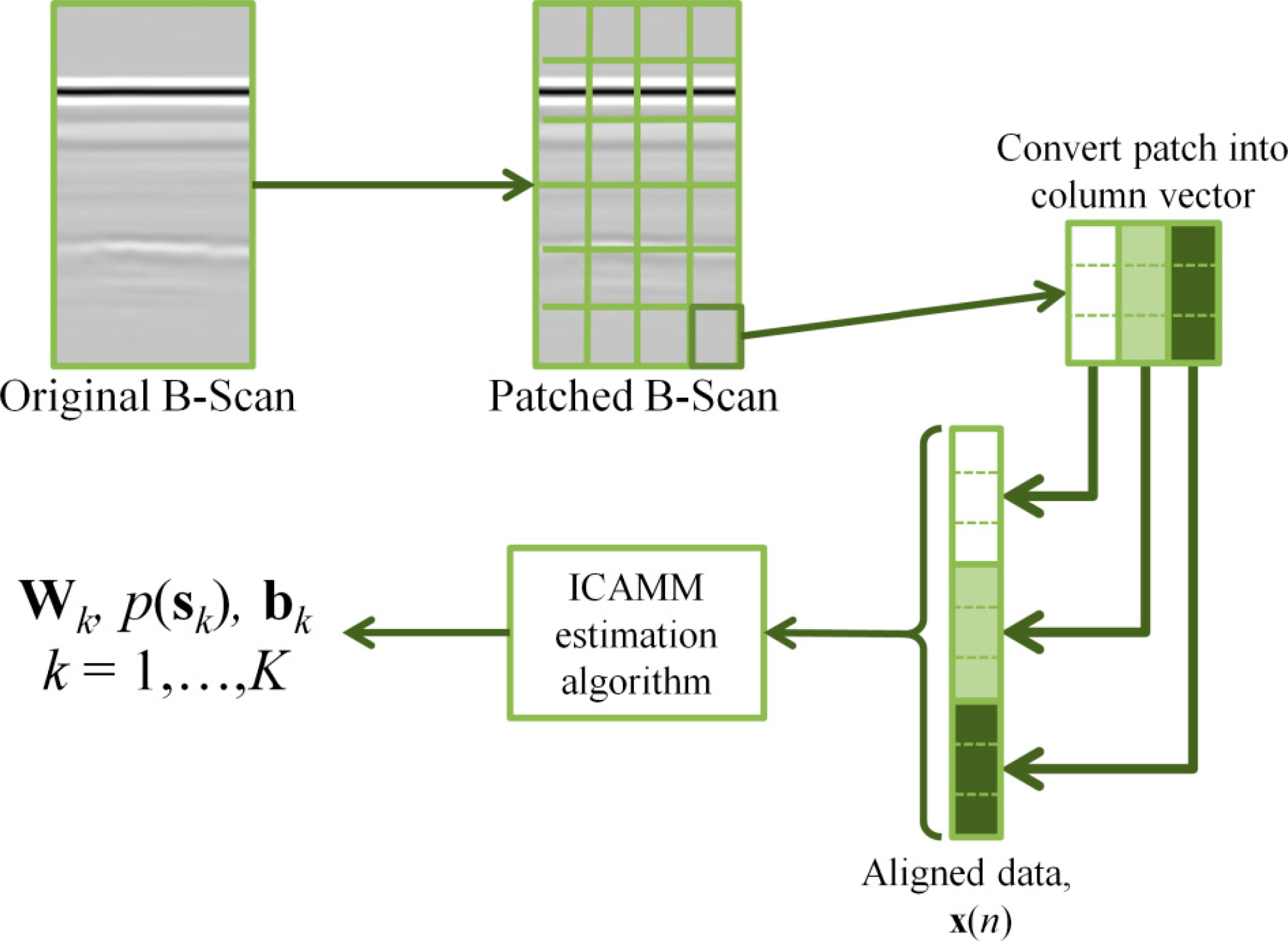
As indicated, Kriging and splines are suited to the processing of spatially-distributed data, such as those obtained in GPR analysis. The other two methods must be adapted to the particular context of GPR data. This was accomplished by following the steps shown in Figure 1. Each B-scan from the GPR signals is divided into squares of fixed size or “patches”. Thus, if the size of a patch is [L × L], each patch comprises L consecutive time samples from L adjacent traces. Then, each patch is transformed into a column vector with M = L2 components by vertically concatenating the columns of the patch. Each one of these vectors is considered an observation x. In this paper, this preprocessing is called “alignment.” The definition of the partition of known and unknown data x = [yTzT]T depends on the particular experiment, as shown in the following sections.
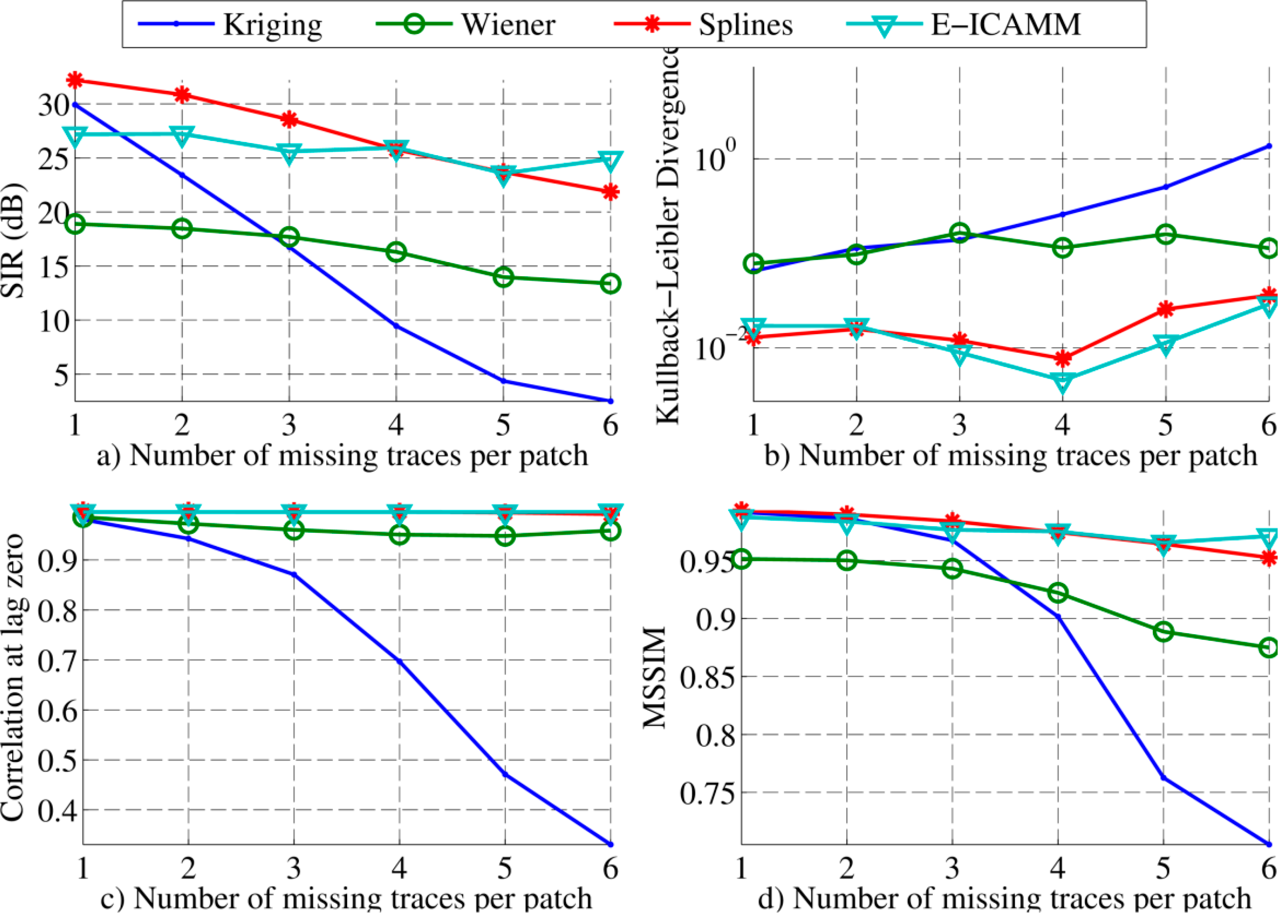
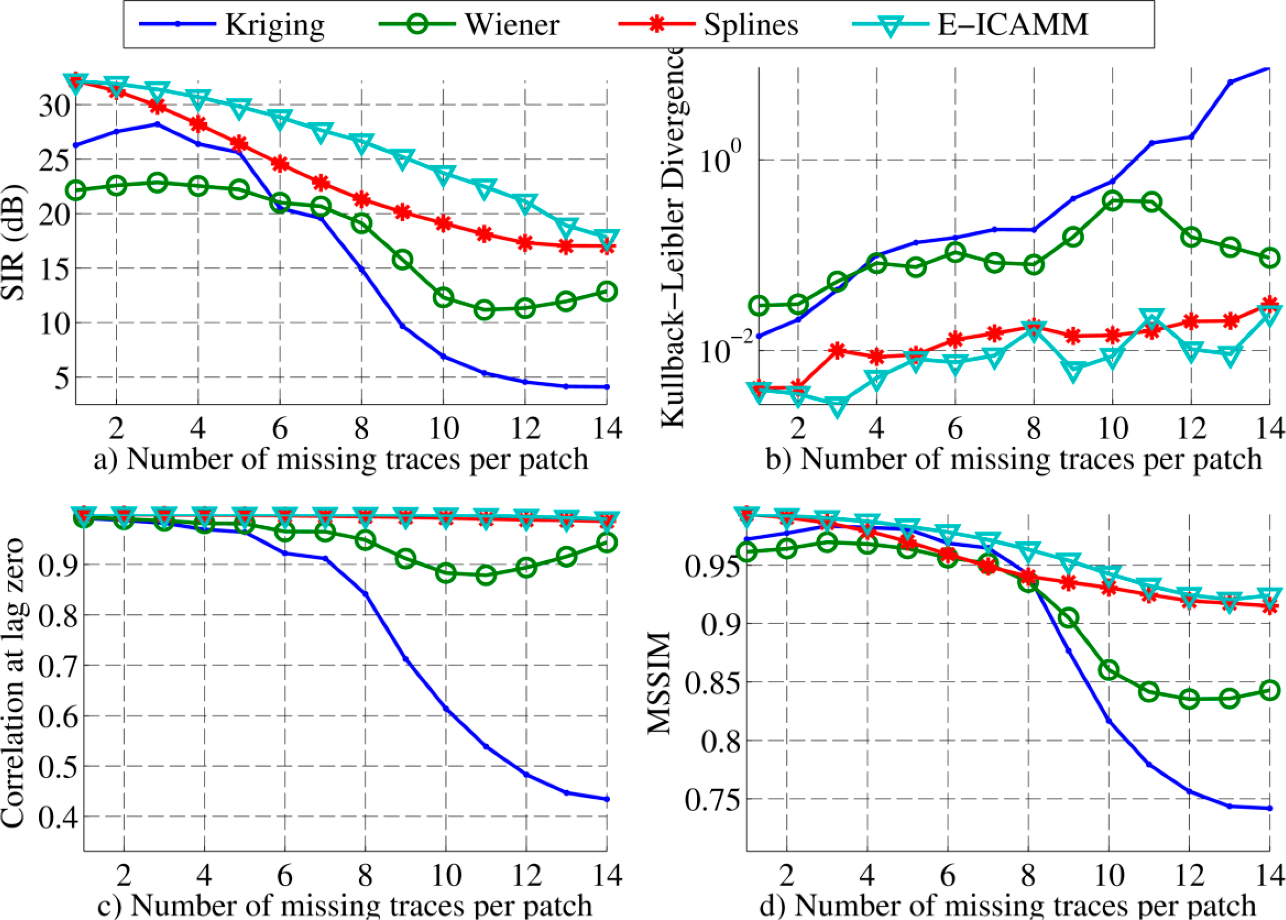
The quality of the estimation yielded by each method can be measured with a variety of performance indicators. We have selected the following four indicators: (1) the signal to interference ratio (SIR, [16]), which measures the sample error; (2) Kullback-Leibler divergence ([17]), which measures the distance between the probability density function of the true data and the predicted data; (3) cross-correlation at lag zero ([18]), which measures the temporal and spatial similarity between signals; and (4) mean structural similarity (MSSIM, [19]), an index commonly used in image processing that measures the structural similarity between two images. These indicators are defined in Appendix B.
Uncertainty, Accuracy and Error
We will now briefly consider the behavior of the proposed methods and error indicators with respect to interpolation accuracy, error and uncertainty. The careful analysis of the dependence of these values on the proposed methods is a complex task, and it is outside of the scope of this study. However, some significant conclusions are possible about these issues, as given in the following. Thus, Kriging predicts missing data using neighboring values and the spatial covariance function. This covariance is usually estimated by fitting a model to known data, and its correct estimation determines the accuracy of the interpolated data. Furthermore, Kriging is known to over-smooth data as the number of missing values (or the distance to the known values) increases [8], also decreasing the accuracy of the model.
The properties of a Wiener structure depend on those of the algorithm used for the linear stage of the structure. Aside from that, the estimation of the nonlinear function can also affect the performance of the Wiener structure [9]. Smaller estimation windows increase interpolation accuracy at the cost of increasing uncertainty, since the correction can change rapidly for similar outputs of the linear stage. The nonlinear correction stage is immune to the number of missing values, because each missing value is treated separately.
Splines calculate the smooth polynomial curve that fits the known data values with minimum energy. The performance of the interpolation depends on the order of the polynomials and the smoothing parameter. Since third-order polynomials are commonly used, the smoothing parameter reduces uncertainty at the cost of some accuracy. The error can increase with the number of missing values, although it depends on the variation between known values. If these variations are close to the function with minimum energy, the error will be low. Conversely, if the variations deviate from said function, the error will increase.
Unlike the previously-presented methods, E-ICAMM has an iterative stage (see Equation (A8) in Appendix A). In practice, however, one iteration is enough to provide a good result. The method always converges after one step to the same result, removing any possible uncertainty in the result. Since it is an LMSE method, the interpolation accuracy of E-ICAMM is usually high. Furthermore, the method is highly resistant to the number of missing values, because the structure of the data is captured in the ICAMM. Although the result is not independent from the number of missing data, it is more robust in this regard than Kriging and splines. The selection of the number of classes and the ICA estimation algorithm affects the interpolation performance of E-ICAMM.
Of all proposed error indicators, the SIR and the Kullback–Leibler divergence (KLD) are the ones that most closely measure the accuracy and the uncertainty in the interpolated results. The correlation and the MSSIM are more sensitive to the spatial structure of the data. Since the SIR is inversely proportional to the mean squared error, it is inversely proportional to the accuracy and the error. The KLD measures the difference between probability densities. The error, uncertainty and accuracy affect the probability density of the interpolated data, which, in turn, increases the KLD with respect to the true data.
3. Results and Discussion
The synthetic GPR data were obtained from the simulation of the 2D model shown in Figure 2a. This model was a homogeneous wall surrounded by air with five discontinuities inside the wall. This model was designed so that it was similar to the real data. The simulated radargram was obtained by applying a ray tracing algorithm in MATLAB®. The resulting B-scan is shown in Figure 2b. The wall had dielectric permittivity εr,ground = 8 (e.g., old cement), and the discontinuities had dielectric permittivity: εr,1 = εr,4 = 20 (wet cement, in gray in Figure 2a), εr,2 = εr,3 = 1 (air, in black) and εr,5 = 81 (water, in white). The final B-scan had 512 traces, and each trace was 1024 samples long. Other parameters were: inline spacing distance, 5 mm; time sampling period, 10 picoseconds; center frequency of the GPR antenna, 1.5 GHz, with a 1-GHz bandwidth; and signal-to-noise ratio SNR = 30 dB. The SNR corresponds to a low noise signal and was chosen to improve the representation of reflections. The noise was modeled with a K-distribution, because it is often the distribution that best fits radar clutter [20].
Kriging and splines are suited to spatially-distributed data, whereas the other methods discussed in this paper require data alignment. Hence, we considered two patch sizes, [8 × 8] and [16 × 16] samples, which were converted to column vectors of M = 64 and 256 variables, respectively. These patch sizes are typical in image processing applications, particularly [8 × 8], which gained popularity due to the importance of JPEG compression and other methods related to the discrete cosine transform (DCT). The fast implementation of such methods requires patch sizes that are powers of two [21]. Patch size, however, is usually determined using empirical methods.
It was assumed that l out of every L GPR traces was corrupted or not captured at all in the experiment (l < L). Thus, the proposed prediction methods were used to interpolate missing information in these traces. Such a scenario could arise while increasing the horizontal scanning rate (i.e., the number of “sampled” locations) by interpolating new traces from the available ones; in this case, the new traces can be considered missing traces and can be interpolated. A similar scenario arises when problems during the data measuring process occur; for instance, if the antenna is moved too fast across the surface and the measurement device is unable to take a proper sample of some locations of the underlying terrain. In this case, however, missing traces would be located at random intervals, depending on the speed of the antenna.
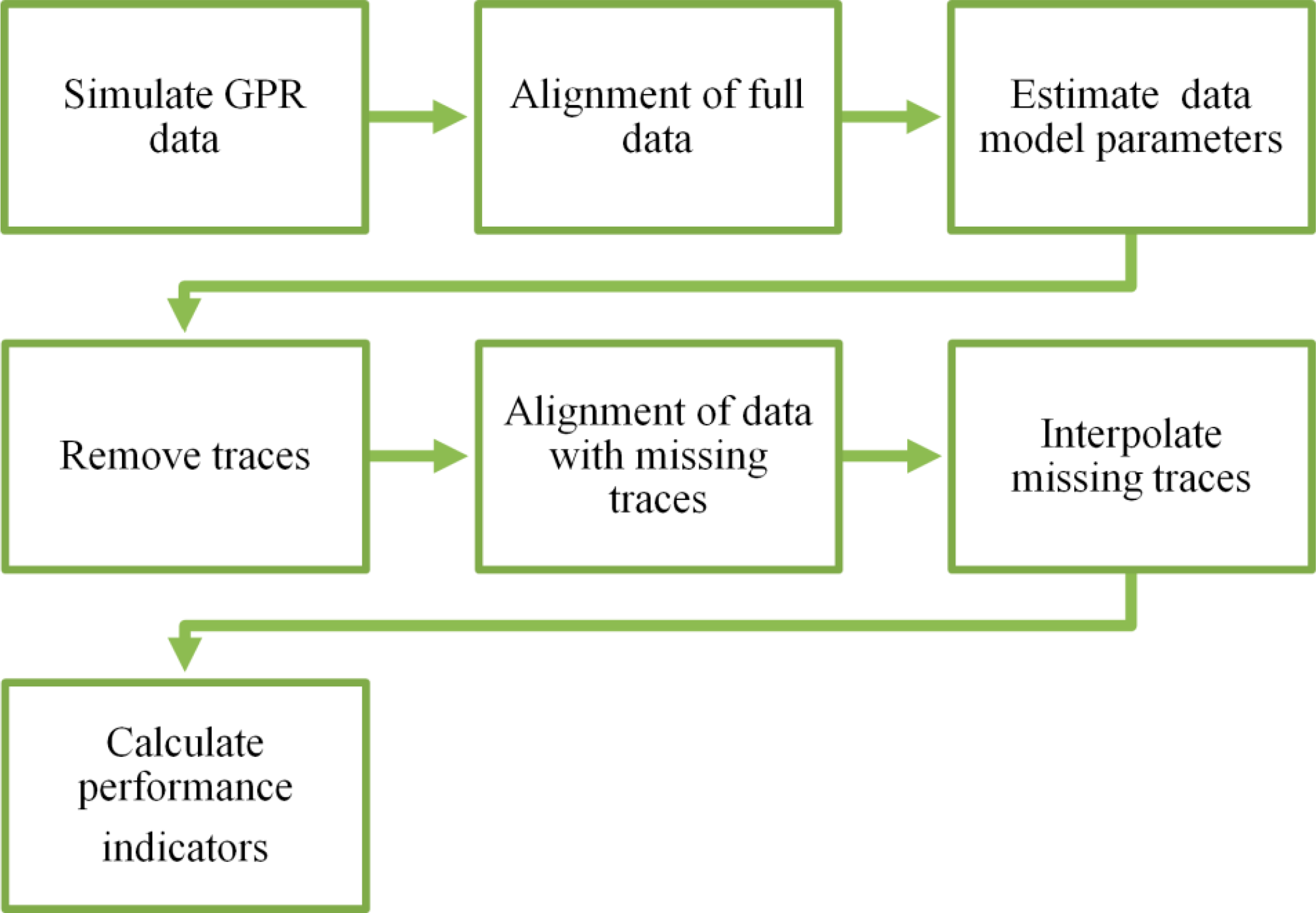
The experimental setup is shown in Figure 3. First, the simulated data are aligned if necessary, and then, any model parameters (such as the covariance function for Kriging or the ICAMM parameters) are calculated from the complete original radargram. In general, the number of classes for ICAMM is determined from the data, either from data with several known classes or by testing several models with an increasing number of classes. Estimation of the ICAMM parameters, however, was a complex process because of the high dimensionality of signals and the high correlation between radargram patches. In the end, we opted for an ICAMM with a single class, whose parameters were found using topographic independent component analysis (TICA [22]). TICA is an ICA algorithm that is commonly used to model natural images, and it employs the same data alignment as that shown in Figure 1.
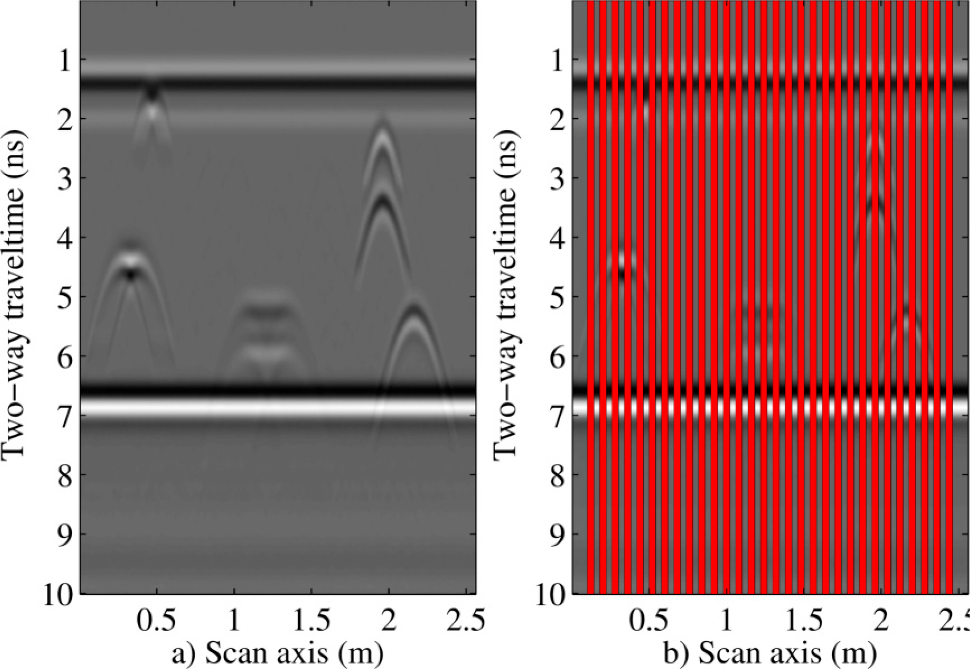
Once the data model parameters required for the implementation of predictors were estimated from the full data, l out of every L traces were marked as erroneous or missing (l < L). The result is shown in Figure 4, where marked traces are marked in red. The equal intervals were selected to obtain an average of prediction performance across the whole B-scan. In practice, local results oscillated near the average values. Marked traces were centered within their patches in order to ensure that there was always some information at the first and last traces of the radargram. This process avoided extrapolation. The missing data were then predicted with each proposed method. Therefore, a substantial number of data were removed from each affected patch, because even a single missing trace caused at least L missing data from every affected patch, where L is eight or 16.
The radargram with missing traces was aligned, and the proposed estimation methods were used to interpolate these erroneous data. Afterward, the similarity between the interpolated data and the true data was measured with the four performance indicators defined in Appendix B: SIR, Kullback-Leibler divergence, correlation at lag zero and MSSIM.
The above experiment was repeated multiple times, each time increasing the number of missing traces around each selected position. The number of missing traces ranged from one to the number of traces per patch minus two (e.g., six traces for [8 × 8] patches). This range was decided to keep at least some information available within every patch.
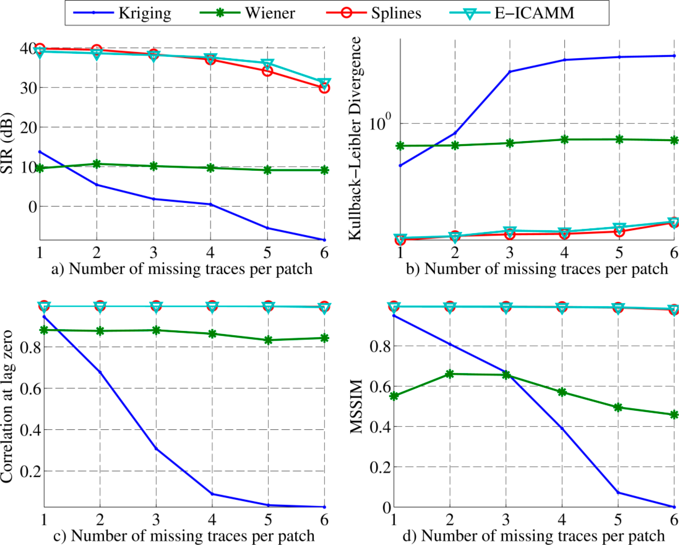
The results for patches of size [8 × 8] are shown in Figure 5. These results can be split into two regions, depending on the amount of reconstructed data. For low amounts of missing traces per patch, splines performed slightly better than E-ICAMM, Kriging obtained the third best result and Wiener structures achieved the worst result. For higher amounts of missing traces, the performance of E-ICAMM matched that of splines and even exceeded it for six missing traces per patch. Furthermore, Wiener structures obtained the third best result when the number of missing traces was high. This performance was owed to the fast worsening of Kriging as the number of missing traces increased, since Wiener structures were more resistant to growth in the amount of unknown data.
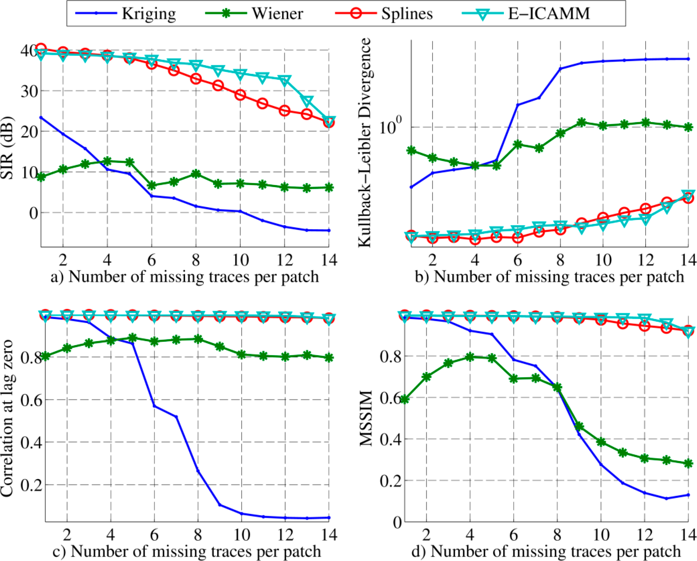
Figure 6 shows the result for patches of size [16 × 16]. E-ICAMM improved its performance with higher patch size, and the other methods obtained similar results as for the [8 × 8] size experiment. E-ICAMM obtained the best result for all considered amounts of missing traces in SIR, correlation and MSSIM. Splines obtained the second best result, followed by Kriging and then Wiener structures. This result might indicate that the ICA mixture model is more appropriate for [16 × 16] patches.
In terms of processing time, Kriging and Wiener structures are more time-consuming than E-ICAMM and splines, although splines is slightly faster than E-ICAMM. Although the E-ICAMM interpolation itself is faster than splines, E-ICAMM requires a previously-estimated ICAMM, which is a costly procedure. The same ICAMM can be used multiple times, even if the number of missing traces changes or they are moved around, which reduces the difference in computational cost.
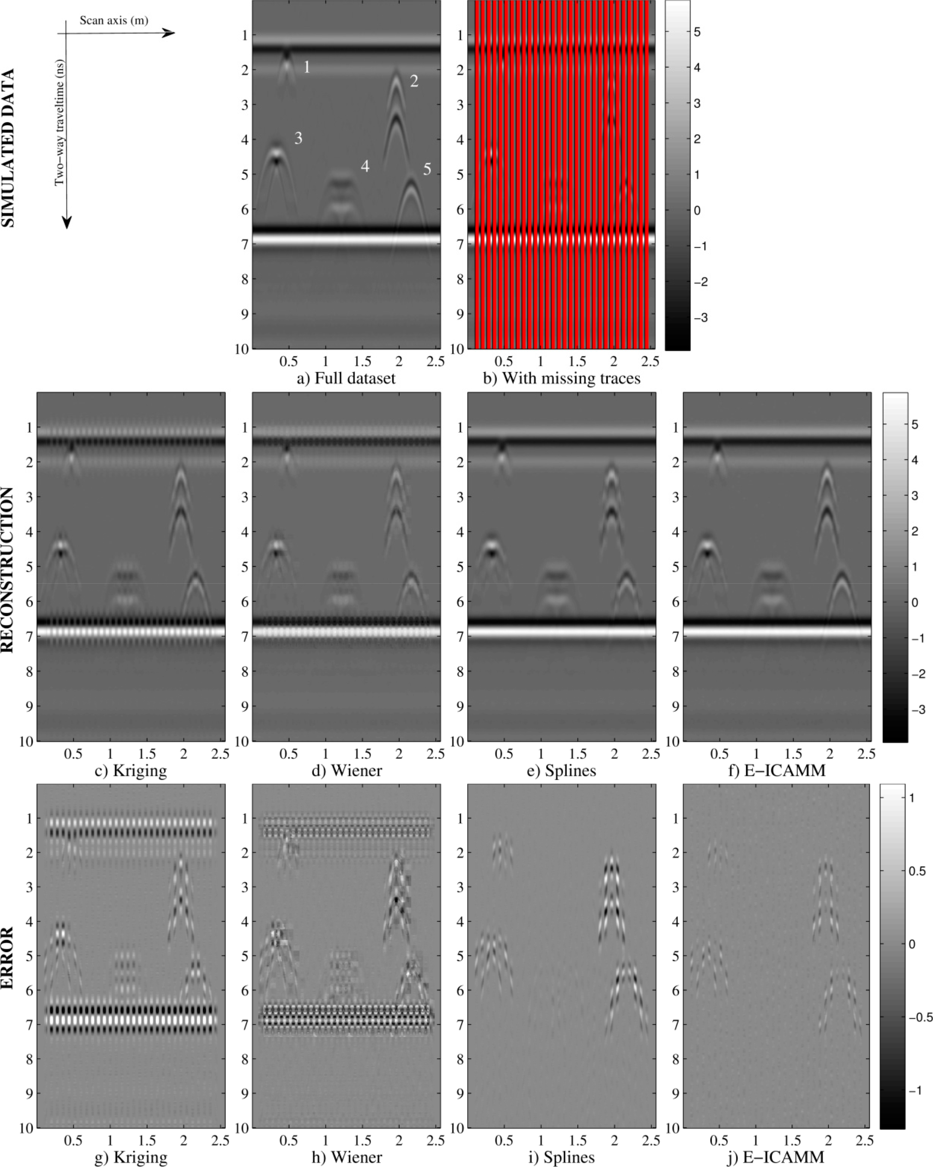
Figure 7 shows the results for [16 × 16] patches with nine missing traces per patch: simulated data (Figure 7a); simulated data with missing traces (Figure 7b); B-scans after interpolation by the studied methods (Figure 7c–f); and prediction error yielded by the studied methods (Figure 7g–j). In concordance with the values in Figure 5, Kriging achieved the worst result, Wiener structures improved with respect to Kriging and E-ICAMM obtained the best quality interpolation, outperforming the results of splines. E-ICAMM and splines both perfectly reconstructed the reflections at the beginning and end of the wall, and the hyperbolas were better reconstructed by E-ICAMM (particularly the hyperbolas for Defects 2 and 5, at the right end of the wall, as depicted by Figure 7).
4. A Real Data Application
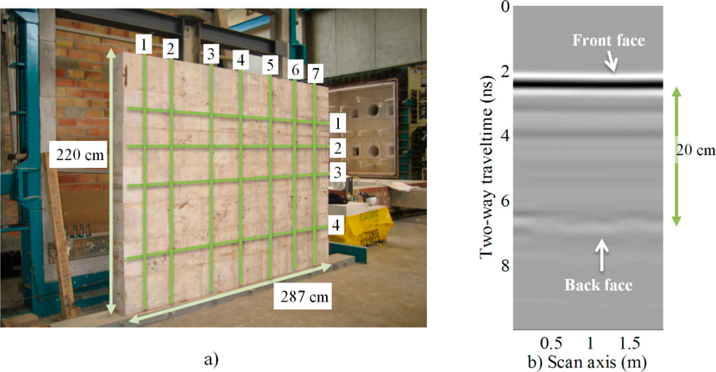
The experiment was carried out on data obtained from a multidisciplinary study on two replicas of historical walls. These data have been used in previous studies [23,24]. Two walls were built in a laboratory to control their composition and introduce certain defects or discontinuities at specific locations. They were built using travertine ashlars from Godella quarry (Spain), and each ashlar was 40 × 30 × 20 cm. The mix was 0:1:3, with no cement and one part sand for every three parts hydraulic lime (NHL5 class). This impoverished mortar is typical of historical buildings and achieves low compressive strength (<4 MPa). The total dimensions of the walls were 287 cm in length, 220 cm in height and 20 cm in thickness. A picture of one of the walls is shown in Figure 8. In order to simulate realistic load conditions, the walls were entered into a hydraulic press set to a pressure of 50 tons.
The GPR equipment consisted of a SIR-3000 data acquisition system and a 1.6-GHz center frequency antenna (model 5100B) from Geophysical Survey Systems, Inc. The dimensions of the antenna were 3.8 × 10 × 16.5 cm. The antenna was fit to an encoder cart built ad hoc for the experiment. The encoder cart was used for two reasons: (1) to ensure a uniform sampling of the wall, capturing data at a constant rate; and (2) to help with the displacement of the antenna across the (uneven) surface of the wall.
Each wall was scanned with the GPR in order to detect any significant flaw, crack or discontinuity. This survey was performed following a grid of trajectories with seven vertical lines and four horizontal lines, placed more or less uniformly along the surface of the wall (see Figure 8a). Thus, in total, 11 B-scans were obtained for each of the two walls. All 11 radargrams were used for this prediction experiment, and the results were averaged. Figure 8b shows an example radargram obtained for vertical radar Line 1 of Figure 8a. Each B-scan was composed of 443 traces, each one 1024 samples long. The inline spacing distance was 6 mm; the time sampling period was approximately 10 picoseconds, and the total time for each trace was 10 nanoseconds.
The procedure was the same as that explained for simulated data; including alignment, interpolation methods and patch sizes. Results for interpolation using [8 × 8] patches are shown in Figure 9. All proposed methods achieved better performance with real data than with simulated data (see Figure 5). This was due to differences in the GPR data. The real data included planar targets (wall discontinuities), and thus, several structures of the real radargrams were spread over many patches, resulting in higher redundancies. Improvement of real data analysis over simulated data was greater for E-ICAMM and splines, which yielded much better results than Kriging and Wiener structures. The performance of E-ICAMM and splines was similar, and E-ICAMM obtained a slightly higher SIR for a high amount of missing traces (see Figure 9a). Wiener structures performed better than Kriging, except for very low amounts of missing traces, indicating a higher presence of nonlinearities in real data with respect to simulated data.
Results for [16 × 16] patches are shown in Figure 10. As with the simulated data, the performance of E-ICAMM was improved with the larger patch size. E-ICAMM and splines performed similarly for low amounts of missing traces, but the relative result of E-ICAMM became better for higher concentrations of missing traces per patch. This is more noticeable in the SIR and MSSIM indicators (Figure 10a,c, respectively). The maximum difference was for the case with 12 missing traces per patch. The difference was lower for 13 and 14 missing traces due to the larger number of missing data in the patch. With 13 or 14 missing traces, the ICAMM no longer had enough information about the structure of the data to reconstruct the signal with high accuracy. The performance of Kriging and Wiener structures was similar to their performance for [8 × 8] patches (Figure 9).
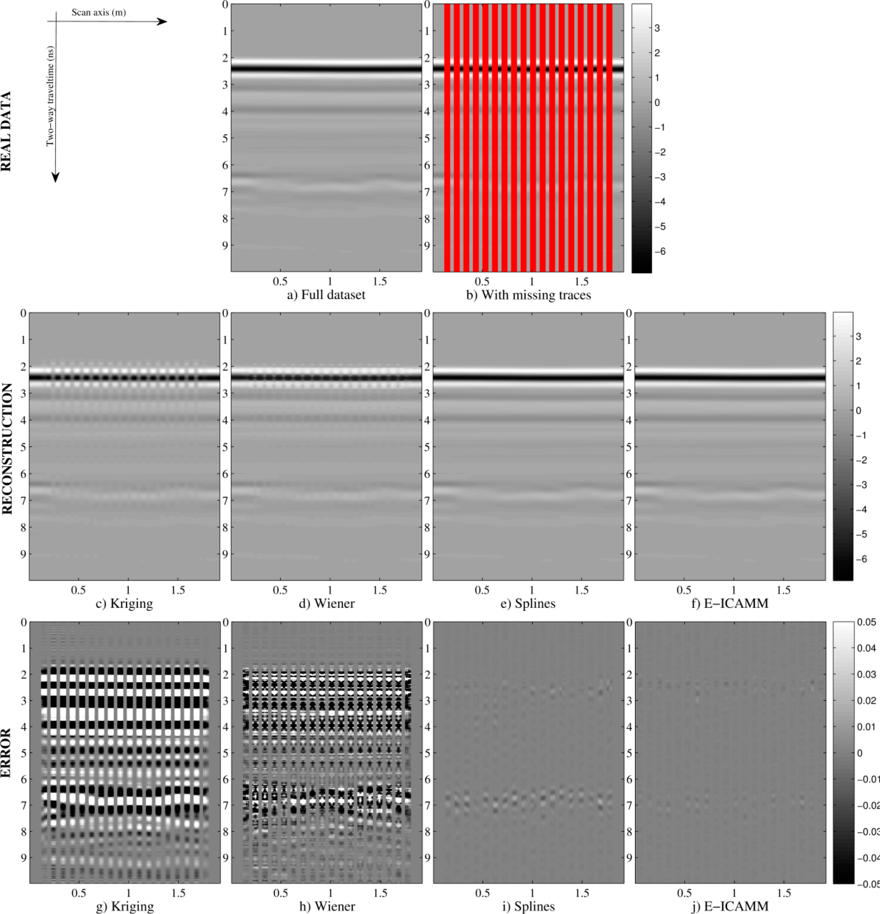
Figure 11 shows the following B-scans: simulated data, simulated data with missing traces and result and prediction error obtained by the studied methods using [16 × 16] patches, with 10 missing traces per patch. Prediction error results are in accordance with the indicators in Figure 10. The highest errors are for interpolation using Kriging and Wiener structures methods; splines performed better than Kriging and Wiener structures; and E-ICAMM achieved the best interpolation (i.e., minimum prediction error), outperforming the other methods. The error was higher around the borders of the wall. This effect was more marked for splines and E-ICAMM (Figure 11e, 11f, respectively). Error for E-ICAMM is negligible, however, and the reconstruction is very close to the real data, even more so for the inside of the wall.
As for the processing times for each method, results were almost identical to those for the simulated data.
To extend the testing of the proposed methods in an application-oriented context, we performed a simple detection experiment on the real radargrams. The radargrams from Wall 2 were used to detect two discontinuities within the wall. The first one was a hollow filled with cement near the upper-left corner of the wall, of a size of 8 × 6 × 2 cm (width, height and length). The second discontinuity was a vertical crack near the right end of the wall, of a size of 0.15 × 5 × 8 cm (width, height and length). The detection algorithm consisted of the following steps: (i) band-pass filtering to remove noise; (ii) background removal using the local mean; (iii) calculation of the envelope of the signals; and (iv) thresholding. This algorithm was valid for our study. Developing an optimum detection algorithm on a set of real GPR data is a challenging task and was therefore beyond the scope of this study.
The detection algorithm was used on the full data set and with the reconstructed results for the case with [16 × 16] patches and 12 missing traces per patch. The detection results, summarized by the area under the ROC (receiver operating characteristic) curve were as follows: 0.6588 (real data), 0.6586 (reconstruction with E-ICAMM), 0.6323 (reconstruction with splines), 0.5546 (reconstruction with Kriging) and 0.5259 (reconstruction with Wiener structures). These areas were calculated for false alarm probabilities between zero and 0.5. E-ICAMM yielded results that were consistently almost identical to those of the data without missing traces. Splines yielded the next best result, and Kriging and Wiener structures yielded the worst detection rates. These results are in concordance with results in Figure 11, showing that a good interpolation can help with subsequent GPR processing steps.
5. Conclusions
We have presented a comparative study of different statistical interpolation methods for recovering missing data in ground penetrating radar (GPR) B-scans (radargrams). The studied methods were the following: two classical methods representative of linear (Kriging) and nonlinear (Wiener structures) interpolators; the standard method used in GPR for interpolation (splines); and a novel method, called E-ICAMM (expectation assuming an independent component analyzers mixture model). E-ICAMM computes the conditional mean of unknown values under the assumption of an underlying independent component analyzers mixture model (ICAMM) for the joint probability densities of the observations. ICAMM is a very general and versatile model, which encompasses the majority of existing statistical models, in particular the classical Gaussian mixture model (GMM). E-ICAMM implements the optimum solution (the conditional mean) under the (highly unrestrictive) constraint of ICAMM. These methods were tested with experiments on simulated and real GPR data.
First, the methods were used to reconstruct missing traces on a set of simulated GPR data. In order to use some of the methods, this application required transformation of the B-scan to a temporal signal by decomposition of the original image into square patches, a process that we have called “alignment.” The results show that splines and E-ICAMM outperformed the classical methods. The relative performance of E-ICAMM and splines depended on the patch size used for alignment. Two patch sizes were considered [8 × 8] and [16 × 16]. In both cases, Kriging yielded the worst result, Wiener structures yielded the second worst result and E-ICAMM and splines yielded the best results. On average, Wiener structures obtained a signal-to-interference ratio (SIR) 2 dB higher than that of Kriging, yet 8–9 dB lower than that of splines and E-ICAMM. The other error indicators showed a similar result. The relative performance of E-ICAMM and splines changed with patch size. For [8 × 8] patches, splines yielded a slightly better result than E-ICAMM (1.4 dB higher SIR on average, with most performance indicators being similar). For [16 × 16] patches, E-ICAMM yielded a consistently better result than splines for all considered indicators, particularly an SIR that was 3 dB better on average. Furthermore, the reconstruction of the proposed method was the best in terms of the shape of the recovered hyperbolas.
In the second experiment, the proposed methods were used to reconstruct missing data from real GPR records based on two replicas of historical walls. This experiment also required the alignment of the data. The interpolation performance in the real radargram was different because of the higher presence of planar targets in the data. The classical methods (Kriging, Wiener structures) decreased their performance with respect to their results for synthetic data (a 9 dB average decrease in SIR), while splines and E-ICAMM both yielded a better result with real data than with synthetic data (8 dB average increase in SIR). Therefore, the difference in performance between the results of splines and E-ICAMM and those of the classical methods was higher for real data than it was for the synthetic radargram. Conversely, the distance between the performance of splines and E-ICAMM was lower than it was for simulated data. For [8 × 8] patches, E-ICAMM obtained a similar result to splines, with an average difference of 0.36 dB in SIR in favor of the former. For [16 × 16] patches, E-ICAMM yielded better results than splines for all considered error indicators, with an average increase in SIR of 2.3 dB. This improvement was more noticeable for a range of missing traces (7–13 errors out of every 16 traces). Notably, the performance of E-ICAMM suffered little decline as the number of missing traces increases, particularly for the case with patch size [16 × 16]. Furthermore, we proved that the improved reconstruction leads to a better detection of discontinuities in the wall. In this task, the reconstruction by E-ICAMM consistently yielded results that approached the quality of results corresponding to the whole data set (without missing traces). In terms of the area under the receiver operating characteristic (ROC) curve, the data interpolated with E-ICAMM yielded a value almost identical to that of the complete (non-interpolated) data set (0.6586 and 0.6588, respectively).
Acknowledgments
This research was supported by Universitat Politècnica de València (Vice-Rectorate for Research, Innovation and Transfer) under Grant SP20120646; Generalitat Valenciana under Grants PROMETEOII/2014/032, GV/2014/034 (Emergent Research Groups), and ISIC/2012/006; and the Spanish Administration and European Union FEDER Programme under Grant TEC2011-23403.
Author Contributions
Gonzalo Safont has contributed with the proposal and implementation of the E-ICAMM algorithm and performance indicators, and obtaining and writing the results of simulations and real experiments. Addisson Salazar and Luis Vergara have contributed with the basis for the E-ICAMM algorithm design, theoretical background, defining of the figures of merit, and the overall proposal and writing of the paper. Alberto Rodriguez has contributed with analyses of the simulations and real experiments.
Conflicts of Interest
The authors declare no conflict of interest.
Appendix A
Let us assume that the joint probability density of the elements of vector x can be modeled by a mixture model with K classes Ck, k = 1, …, K:
To compute E [z | y, Ck] in the sum, we assume that P (x | Ck) follows an ICA model,
Given the known value y, Equation (A6) represents an overdetermined linear system of equations, which can be solved in the unknown E [z | y, Ck], using, for example, the pseudoinverse .
This requires knowledge of E [sk|y, Ck]. We have considered an iterative algorithm, which iteratively computes E [z | y, Ck] and E [sk | y, Ck], namely:
Results in this paper correspond to only one iteration (I = 1), because no significant improvements were observed for more than one iteration.
This is repeated for every class to obtain the values E [sk | y, Ck], k = 1, …, K required in Equation (A3). We also need to compute P (Ck | y), k = 1, …, K. Using Bayes rule:
Appendix B
Four error-performance indicators were selected to evaluate the quality of each interpolation method. A brief definition and explanation of them follows. We will call ẑ the estimate of the true value z computed by any of the four methods.
Signal-to-Interference Ratio
The first indicator chosen was the signal-to-interference ratio (SIR), a commonly-used performance indicator [16]. It is defined as:
Kullback-Leibler Divergence
The second performance indicator is the Kullback-Leibler divergence (KLD), a classical indicator of distance between two probability distribution functions [17]. In this case, we computed the distance between the densities of the predicted data (pẑ(v)) and that of real data (pz(v)). A symmetrized version of the indicator was used:
Cross-Correlation at Lag Zero
Cross-correlation (CORR) at lag zero is a classical similarity measure between two sequences of numbers [18]. It can be defined in different related forms. Here, we define it as:
Structural Similarity Index
The fourth performance indicator is the structural similarity index (SSIM), an indicator of similarity between two images [19], which can be applied to the comparison between two vectors. This is performed first at a local level, by comparing the differences in “luminance”, “contrast” and “structures”, corresponding to every couple zm, as defined by the following equations:
The local SSIM is calculated as:
References
- Daniels, D.J. Ground Penetrating Radar; The Institution of Engineering and Technology: London, UK, 2004. [Google Scholar]
- Cassidy, N. Ground penetrating radar data processing, modelling and analysis. In Ground Penetrating Radar Theory and Applications; Jol, H.M., Ed.; Elsevier: Amsterdam, The Nederlands, 2009; pp. 141–176. [Google Scholar]
- De Boor, C. A Practical Guide to Splines; Springer: New York, NY, USA, 1987. [Google Scholar]
- Strange, A. Analysis of time interpolation for enhanced resolution GPR data. In Proceedings of the 7th International Workshop on Advanced Ground Penetrating Radar, Nantes, France, 2–5 July 2013.
- Le Bastard, C.; Baltazart, V.; Wang, Y.; Saillard, J. Thin-pavement thickness estimation using GPR with high-resolution and superresolution methods. IEEE Trans. Geosci. Remote Sens 2007, 45, 2511–2519. [Google Scholar]
- Windsor, C.G.; Capineri, L. Automated object positioning from ground penetrating radar images. Insight 1998, 40, 482–488. [Google Scholar]
- Schafer, R.W.; Rabiner, L.R. A digital signal processing approach to interpolation. Proc. IEEE 1973. [Google Scholar] [CrossRef]
- Surhone, L.M.; Timpledon, M.T.; Marseken, S.F. Spatial Descriptive Statistics: Descriptive Statistics, GIS, Geostatistics, Variogram, Correlogram, Kriging, Cuzick-Edwards Test; VDM Publishing: Saarbrücken, Germany, 2010. [Google Scholar]
- Wang, J.S.; Hsu, Y.L. Dynamic nonlinear system identification using a wiener-type recurrent network with OKID algorithm. J. Inf. Sci. Eng 2008, 24, 891–905. [Google Scholar]
- Micula, G.; Micula, S. Handbook of Splines; Springer: Amsterdam, The Nederlands, 1999. [Google Scholar]
- Vaseghi, S.V. Advanced Digital Signal Processing and Noise Reduction, 3nd ed; Wiley: Sissex, UK, 2006. [Google Scholar]
- Scharf, L.L. Statistical Signal Processing: Detection, Estimation and Times Series Analysis; Addison-Wesley: Boston, MA, USA, 1991. [Google Scholar]
- Journel, A.G.; Huijbregts, C.J. Mining Geostatistics; The Blackburn Press: West Caldwell, NJ, USA, 2004. [Google Scholar]
- Salazar, A.; Vergara, L.; Serrano, A.; Igual, J. A general procedure for learning mixtures of independent component analyzers. Pattern Recognit 2010, 43, 69–85. [Google Scholar]
- Bishop, C.M. Pattern Recognition and Machine Learning; Springer: New York, NY, USA, 2006. [Google Scholar]
- Vincent, E.; Gribonval, R.; Févotte, C. Performance measurement in blind audio source separation. IEEE Trans. Audio Speech Lang. Process 2006, 14, 1462–1469. [Google Scholar]
- Kullback, S.; Leibler, R. On information and sufficiency. Annals of Mathematical Statistics 1951, 22, 79–86. [Google Scholar]
- Orfanidis, S. Optimum Signal Processing: An Introduction; Prentice-Hall: Upper Saddle River, NJ, USA, 1996. [Google Scholar]
- Wang, Z.; Bovik, A.; Sheikh, H.; Simoncelli, E. Image quality assessment: From error visibility to structural similarity. IEEE Trans. Image Process 2004, 13, 600–612. [Google Scholar]
- Raghavan, R. A model for spatially correlated radar clutter. IEEE Trans. Aerospace Electron. Syst 1991, 27, 268–275. [Google Scholar]
- Li, X. Patch-based image processing: From dictionary learning to structural clustering. In Perceptual Digital Imaging: Methods and Applications; Lukac, R., Ed.; CRC Press: Boca Raton, FL, USA, 2012; pp. 223–250. [Google Scholar]
- Hyvarinen, A.; Hoyer, P.; Inki, M. Topographic independent component analysis. Neural Comput 2001, 13, 1527–1558. [Google Scholar]
- Safont, G.; Salazar, A.; Vergara, L. Detection of imperfections within historic walls using ground-penetrating radar. In Proceedings of the 10th International Conference on Computational and Mathematical Methods in Science and Engineering, Almería, Spain, 26–30 June 2010.
- Salazar, A.; Safont, G.; Vergara, L. Application of independent component analysis for evaluation of Ashlar Masonry Walls. Lect. Notes Comput. Sci 2011, 6692, 469–476. [Google Scholar]

© 2014 by the authors; licensee MDPI, Basel, Switzerland This article is an open access article distributed under the terms and conditions of the Creative Commons Attribution license (http://creativecommons.org/licenses/by/3.0/).
Share and Cite
Safont, G.; Salazar, A.; Rodriguez, A.; Vergara, L. On Recovering Missing Ground Penetrating Radar Traces by Statistical Interpolation Methods. Remote Sens. 2014, 6, 7546-7565. https://doi.org/10.3390/rs6087546
Safont G, Salazar A, Rodriguez A, Vergara L. On Recovering Missing Ground Penetrating Radar Traces by Statistical Interpolation Methods. Remote Sensing. 2014; 6(8):7546-7565. https://doi.org/10.3390/rs6087546
Chicago/Turabian StyleSafont, Gonzalo, Addisson Salazar, Alberto Rodriguez, and Luis Vergara. 2014. "On Recovering Missing Ground Penetrating Radar Traces by Statistical Interpolation Methods" Remote Sensing 6, no. 8: 7546-7565. https://doi.org/10.3390/rs6087546
APA StyleSafont, G., Salazar, A., Rodriguez, A., & Vergara, L. (2014). On Recovering Missing Ground Penetrating Radar Traces by Statistical Interpolation Methods. Remote Sensing, 6(8), 7546-7565. https://doi.org/10.3390/rs6087546


