Small-Scale Surface Reconstruction and Volume Calculation of Soil Erosion in Complex Moroccan Gully Morphology Using Structure from Motion

 ,
,
Abstract
: This study presents a computer vision application of the structure from motion (SfM) technique in three dimensional high resolution gully monitoring in southern Morocco. Due to impractical use of terrestrial Light Detection and Ranging (LiDAR) in difficult to access gully systems, the inexpensive SfM is a promising tool for analyzing and monitoring soil loss, gully head retreat and plunge pool development following heavy rain events. Objects with known dimensions were placed around the gully scenes for scaling purposes as a workaround for ground control point (GCP) placement. Additionally, the free scaling with objects was compared to terrestrial laser scanner (TLS) data in a field laboratory in Germany. Results of the latter showed discrepancies of 5.6% in volume difference for erosion and 1.7% for accumulation between SfM and TLS. In the Moroccan research area soil loss varied between 0.58 t in an 18.65 m2 narrowly stretched gully incision and 5.25 t for 17.45 m2 in a widely expanded headcut area following two heavy rain events. Different techniques of data preparation were applied and the advantages of SfM for soil erosion monitoring under complex surface conditions were demonstrated.1. Introduction
As gullies represent a major sediment source, especially in arid landscapes, many studies examine gully erosion with different approaches [1]. Therefore, no justification is necessary for further effort in improving existing methods for capturing soil erosion processes and their consequences as the demand for measuring techniques of high precision is apparent [2]. While soil scientific analysis, simulated rainfalls or erosion modeling play a major role in erosion research, imaging techniques to reconstruct surfaces and monitor changes are of major importance. A number of studies refer to soil loss quantification by means of remote sensing [3–5]. As computational capacities increase rapidly, recent means in morphological visualization and quantification increasingly complement or replace classical methods. Since it already proved to be a suitable tool in different sciences such as geoarchaeology [6], architecture [7] and robotics [8], this study aims to apply and validate the structure from motion method in soil erosion research. Castillo et al. (2012) already published an accuracy assessment for different field measuring methods in gullies including structure from motion (SfM) [9]. Few studies utilized the emerging terrestrial approach in geomorphology [10] or comparable disciplines to generate terrain models [11].
Especially in difficult to access semi-arid research areas the benefits of the presented method become obvious: logistics and mobility advantages, improved precision compared to established methods and low-cost equipment. While LiDAR represents a major step forward in resolution and accuracy for surface modeling [12,13], it still incorporates inherent disadvantages, e.g., high costs, restricted manageability in rough and inaccessible terrain and required permissions for customs. As the surveyed erosion forms represent a complex and winding morphology, a TLS-system would quickly reach its limits due to either shadowing or a need of too many perspectives [14].
A fast way for scanning extensive surfaces is the use of an unmanned airborne vehicle (UAV) system which is adequate in a lot of morphological surroundings, but is restricted in gullies. An approach by d’Oleire-Oltmanns et al. (2012) [3] makes use of small-format aerial photography (SFAP) for generating digital elevation models (DEM) and calculates lost soil volumes by referring the derived models back to the former land surface. Previously published studies map the amount of headcut retreat and sidewall collapses with high precision UAV surveying. Nevertheless, they remain limited in their abilities to picture different shapes inside the gully and undercuts below the surface [3,15]. A time-consuming part of UAV surveying is the distribution of ground control points (GCPs) and their registration with a total station or a differential global positioning system (dGPS). Even though newly available UAV systems are already capable of locating their position with an onboard dGPS unit, they remain costly and entail the above-described restrictions. Thus, precise volume definition from airborne platforms remains hardly feasible as small-scale obstacles, undercuts, pipes and meanders have a great deal of influence on gully dynamics and the behavior of strong channel runoff [16]. Therefore, it is essential to cover them by 3D surface reproduction.
Over a one-year period with strong rainfall events a measuring campaign to create a time series of surface alteration due to soil erosion was carried out. Images documenting the change on highly degraded soils were used to create high resolution surface models of each time step. In order to further test and demonstrate the abilities of the method for geomorphological issues, to gain information on the precision of SfM measurements and to validate the aforementioned strategy, experiments involving a terrestrial laser scanner (TLS) were facilitated. Hereby, a direct comparison between the scientifically established LiDAR and the ever-expanding structure from motion algorithms and their application in geomorphology was achieved.
The advantages of SfM in geosciences have been demonstrated convincingly by James and Robson (2012) in different scales and applications [17]. Yet, the study presented here demonstrates a non-GCP approach to distinctly reduce working time by putting objects of known sizes into the scene for later scaling of the model and relinquishes UAV data. Thus, the study aims to show the capabilities of terrestrial structure from motion in comparison to TLS as a low-cost and agile tool in a geomorphologic complex surrounding with distinct changes in a one-year erosion monitoring setting from March 2012 to March 2013.
2. Research Areas
Two research areas will be presented in the following chapter: the Souss Valley in Morocco represents a morphologically active region with immanent and striking gully growth and soil degradation. These ever-changing soil surfaces were measured and monitored with the here presented SfM technique. The second experimental site in a quarry near Eichstätt served as a field laboratory as it offered appropriate opportunities to validate the results from the Morocco field campaign.
2.1. The Souss Valley, Morocco
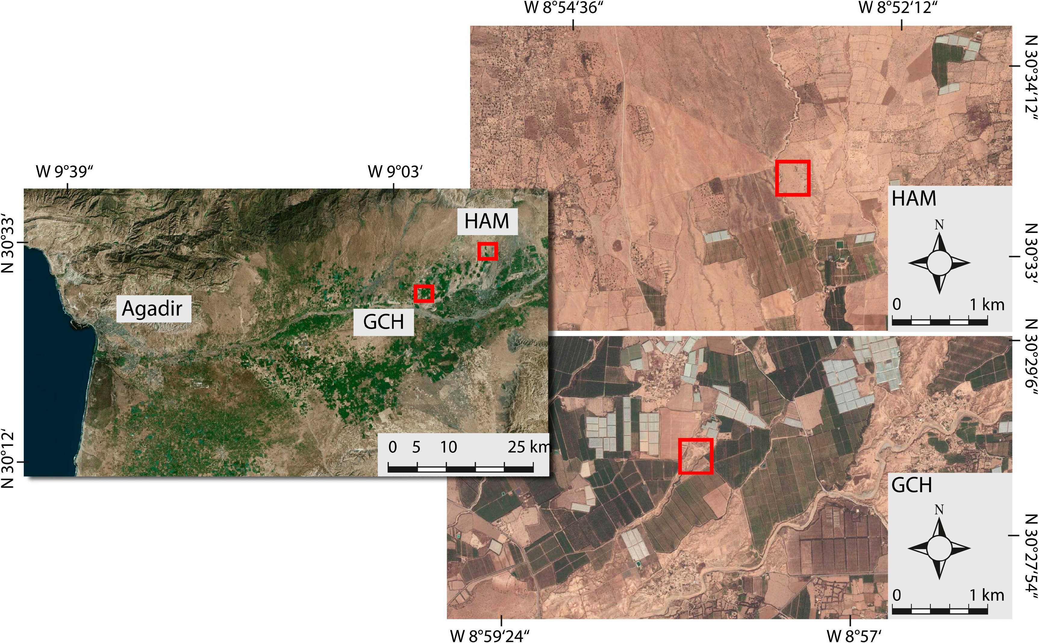
The Souss Valley is located in southern Morocco, east of Agadir, framed by the mountain ranges of High Atlas in the north and Anti Atlas to the south. Its triangle shape extends between a 30° and 31° northern latitude and from a 7° to 9° western longitude (Figure 1, [18]). The plain is described as a transition zone between the Atlantic coastal landscape and the Sahara Desert with the eastern tip around 150 km away from the coast [19]. The research sites Gschechda (GCH) and Hamar (HAM) are situated on a slightly inclined, mainly flat but dissected alluvial fan which drains from the High Atlas mountains in the north to the river Souss in the center of the plain. The fans’ drainage system is highly ephemeral with years without discharge and strong flooding events in the wet season. Due to their alpidic (Cretaceous) overprinting and uplift to above 4100 m (Jebel Toubkal 4167 m), the Palaeozoic, Mesozoic and Cenozoic rocks of the High Atlas Mountains produce vast amounts of sediment. Also, the older Anti Atlas relief, mainly Paleozoic rocks on Precambrian bedrock combined with transgressive sediments, was reactivated by the alpidic uplift causing sedimentation in the southern part of the Souss Valley [20]. The latter again overlay a sequence of older fluvial and lacustrine sediments. The current surface consists of widespread dissected alluvial fans and terraces that were object to recent research [21]. The deepened base level of erosion is a result of the incised oueds (Arabic term for dry riverbeds that show temporal runoff following heavy rain events), which further increases the dissection of the soil surface as a result of locally increasing relief intensity. The aforementioned research sites are situated in a strongly dissected distal part of an alluvial fan northwest of the city of Taroudannt. The negative water balance (212 mm average annual precipitation, mean temperature of 20 °C) and the long and dry summer put drought stress on the mainly agriculturally used vegetation that requires massive irrigation from aquifer wells. Thus, the wet season between October and March is of major importance for groundwater recharge. Rain events are characterized by a high variability during the mild winter and can produce annual amounts in a few days [22,23]. A high content of soda was shown by our own laboratory analysis, resulting in low aggregate stabilities. Calcium carbonate and gypsum accumulations are allocated throughout the research sites. Further field observations lack clear genetic horizons in the alluvial and colluvial soils supplemented with the aforementioned laboratory experiments, thereby leading to classifying the soils as sodic regosols.
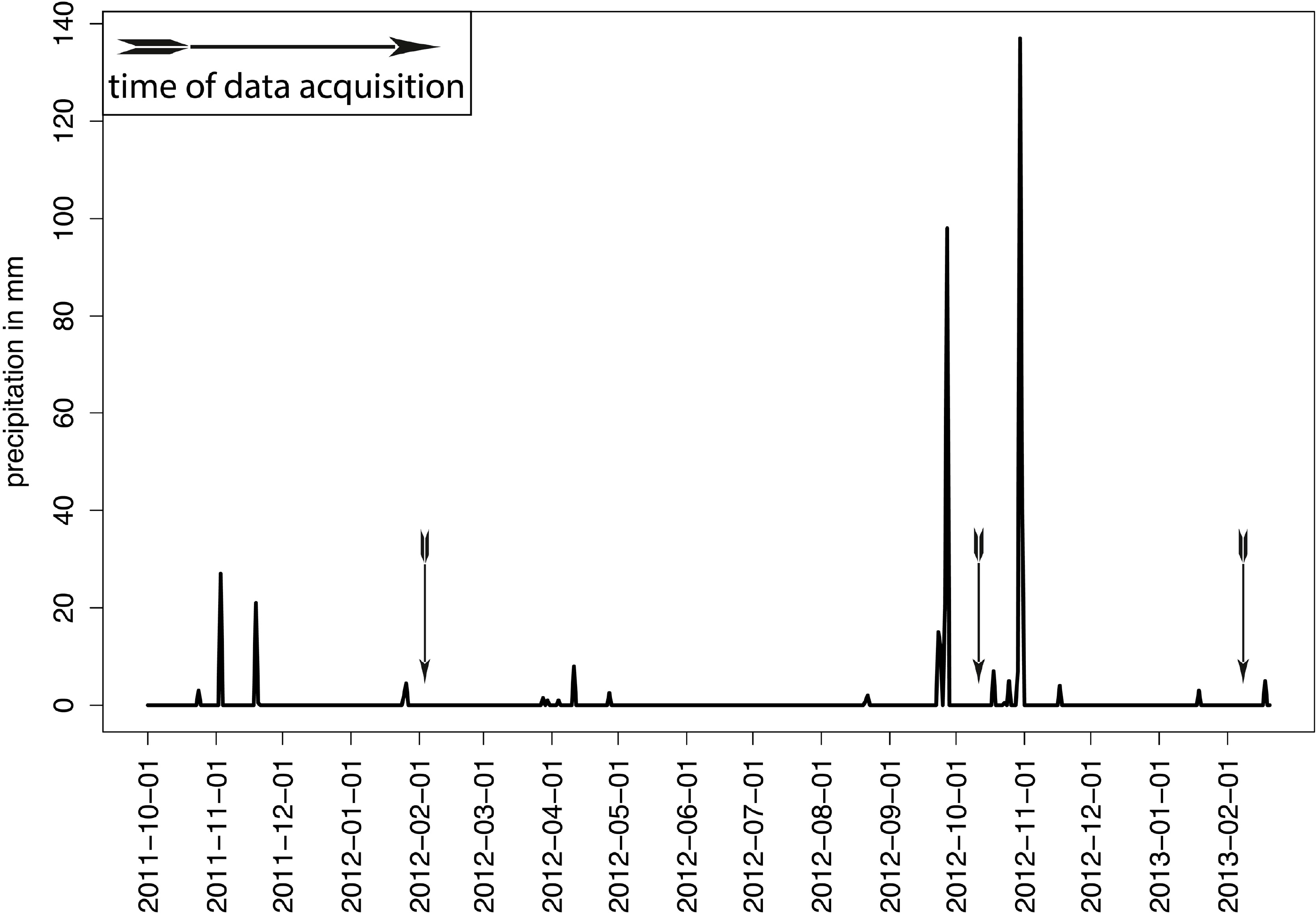
As a major production site for agro-industrial exports in northwestern Africa, constant high pressure weighs on soil and water resources of the region. Especially soil erosion, as in many semiarid regions worldwide, represents a widespread phenomenon to a striking extent. Gully growth by retreating headcuts and sidewall collapses of existing wadis damage infrastructure, thus affecting both plantation owners and residents. Costly land-levelling measurements are implemented to reclaim arable land which was already lost to water-induced erosion. The success of recapturing degraded badlands or gully systems is highly questionable and leads to an increase in soil loss on the reshaped surface [24]. Reoccurring, existing or newly developing gully systems and rill structures represent complex morphological appearances with high dynamic development during the wet season in winter. During the measuring period from March 2012 to March 2013, exceptionally strong precipitation events occurred in the Souss Valley causing severe damage to infrastructure (Figure 2).
2.2. Quarry Site, Eichstätt, Germany
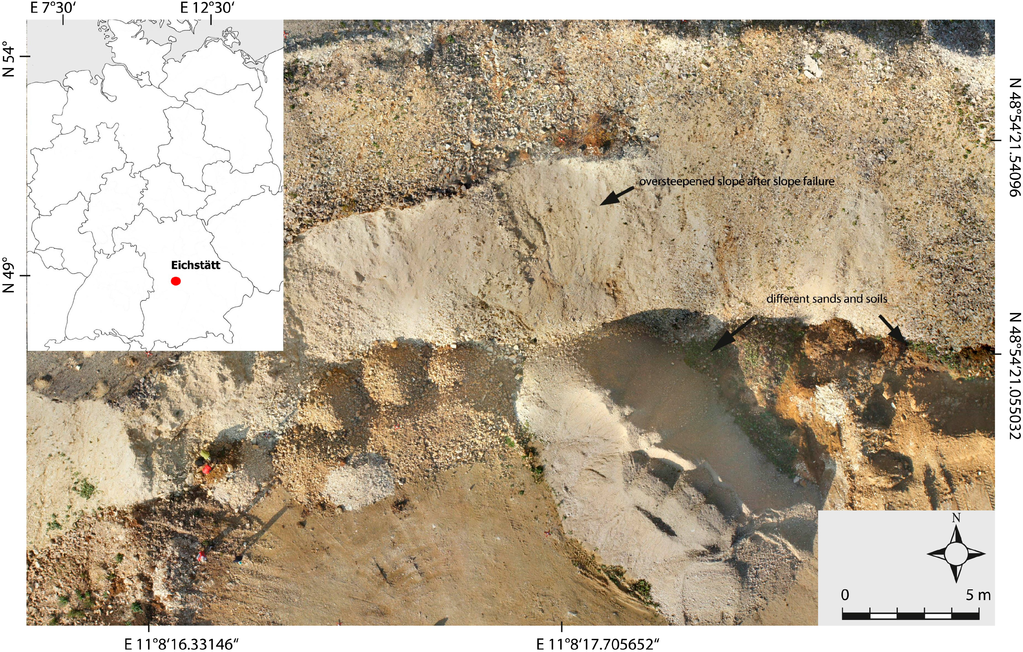
A limestone quarry a few kilometers away from Eichstätt, Bavaria serves as a field laboratory (Figure 3). The quarry is easily accessible and equipped with several permanently fixed reflectors, serving as tie points (e.g., for TLS) and a climate station.
Dumped Jurassic lithological limestone particles as excavated from the quarry form steep hills with slopes exceeding 60° in some parts. Slope failures lead to oversteepened slopes. The quarry is additionally serving as a deposit for other earthy materials (e.g., sands and soils). Major differences in slope length, slope gradient and materials enable the observation and reproductions of a wide range of slope morphological processes.
3. Methodology
3.1. Preface—Structure from Motion and Terrestrial Laser Scanning
3.1.1. Image Acquisition for Structure from Motion (SfM)
The SfM technique is based on computer visualization techniques and picture-based 3D-surface reconstruction algorithms [25]. It provides a means to produce highly detailed models by applying a nonmetric and commercially available digital camera—in this study a Canon EOS 350D—to take images from a multitude of perspectives of any given object.
A lens (Tamron SP AF 17–50 mm 2.8) with a short focus of 0.27 m and suitable sharpness at lower light conditions at wide aperture (f/2.8) was chosen to guarantee enough detail in dark undercuts or a plunge pool. The use of a flash is not recommendable as direct light has negative influence as will later be described. Depending on the complexity and extent of the shape in question, between 40 and 600 handheld images were taken with a sufficient overlap and a planned walking path. A recommended overlap as in aerial photography of around 60% sideways and 80% in moving direction [26] is hardly comparable to the overlap in terrestrial imagery. In aerial photography, the distance of the camera system to the object of interest and the perspective remain more or less stable despite the moving aircraft. However, during terrestrial image acquisition for SfM, the camera moves around the object with almost randomly changing angles and distances. Estimating the thus produced overlap is of little expedience. In specific morphologic situations and erosion process-related appearances of a gully, the density of images was increased to gain further details. It is important to note that there is no direct correlation between image count and detail of the model as certain images might not contain additional information for the final model. This is highly dependent on extra perspectives. Thus, any certainty on the required minimum number of images is impossible. The user will decide on the image count according to the desired resolution of the model, the complexity of the terrain and its accessibility, and the available hardware performance. Experience in applying the technique reduces the image number without deteriorating the final model by a well-chosen distribution of perspectives. In order to scale the models, objects of known dimensions (box, wooden square, geometer) were placed and well distributed in the setup and are also included in the produced 3D model. Thus, chosen perspectives need to include these objects to allow for high precision in the scaling process.
As a prerequisite for adequate results, camera movement between each photo is mandatory. Fixed camera installation on a moveable crane or a tripod might reduce the number of shots and perspectives as a result of repeated erection. This would negatively influence the result of the SfM workflow. Handheld capturing is the easiest and fastest way. Lens distortion towards the very wide-angle (fisheye) lenses can produce a lower recognition rate of features which has to be adjusted prior to processing using Brown’s distortion model [27]. Especially in close range photogrammetry, these system internal calibration parameters need to be taken care of. Lens distortion has a major influence on the quality of the modeling results. Any variation of a straight line of the projection between object and sensor is attributed to radial distortion and leads to a misalignment of image attributes. Parameters of radial distortion are K1, K2 and K3; tangential distortion is given by P1 and P2 [28] and can be determined with open source software such as Agisoft Lens (Table 1) [29]. To gain calibration data, a chessboard pattern is displayed on screen that is then photographed with the lens in use during field work at the same focal length. Especially for wide-angle lenses, the offset of vertical and horizontal lines is visible and used for the automatic calibration in Agisoft Lens. Derived data is then exported in .xml format and used as correction coefficients for the model building process in Agisoft’s Photoscan [30]. Redundant or blurred images can be visually deselected in advance to accelerate workflow.
3.1.2. SfM Point Cloud and Mesh Generation
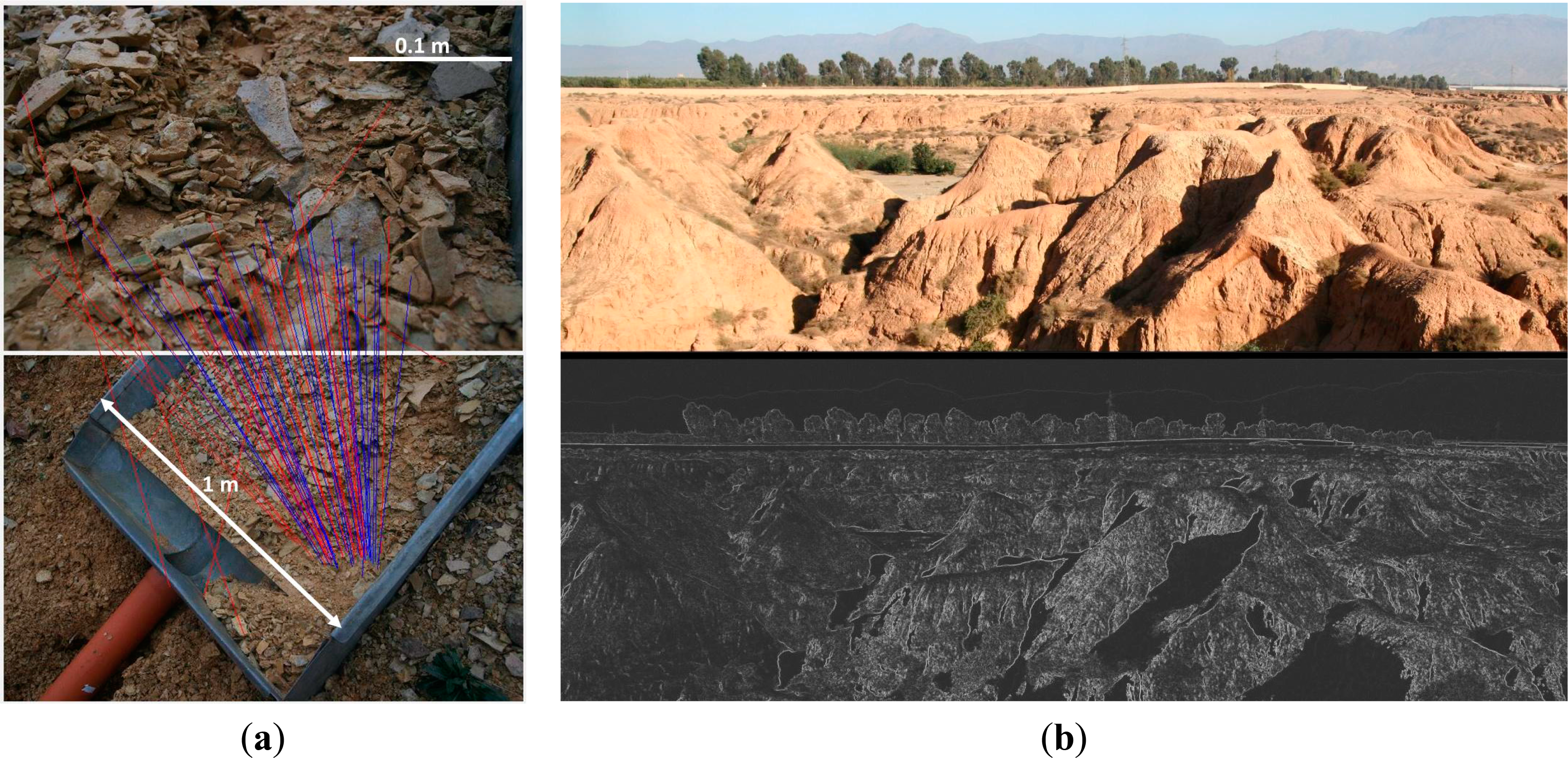
The reproduced complexity causes a rethinking in data treatment as undercuts, plunge pools and piping outlets overburden the established raster data used in GIS-processing. The latter is a result of the ability to exclusively handle non-ambiguous z-values in a grid. A more suitable tool is point clouds whose points represent nodes, so called vertices, for generating a 3D-mesh. The higher the point count, the more detailed the reconstruction of the surface. Depending on size and desired resolution, the point density can exceed the LiDAR data by one order of magnitude. As an output of both laser scans and structure from motion data acquisition, point clouds offer a great amount of information, which is frequently underestimated in research. In a first step, the images are scanned for tie points which represent points in the image that will be retrieved in other pictures. In Figure 4a, an example of point detection is shown. Red lines show erroneously detected feature points; the blue ones could be confirmed by other images. A solution to the required feature detection in multiple images and the matching of their respective 3D locations is realized by a Scale-Invariant Feature Transform (SIFT) algorithm [31] in open source software. Agisofts Photoscan uses comparable algorithms with higher alignment capabilities and was therefore used throughout this study. Feature detection profits from corner and edge detection which again relies on clear contrast differences. Therefore, any surface of low contrast causes trouble to the detection algorithms. On natural surfaces this could not be witnessed, but objects like boxes or metal plot boundaries produce errors in the model. The detected features are invariant to image scaling (e.g., zoom or close- and wide-range imagery), camera rotation and to a certain degree to illumination changes. An example for challenges with the latter can appear in semiarid landscapes with light soils and direct sunlight (Figure 4b), as shadows can result in false edge detection.
Hence, optimum conditions for point detection are granted under diffuse lighting and overcast sky. The latter was challenging in the dry Souss Valley, but is could have possibly been due to dust in the air. The resulting three-dimensional point clouds generated from Agisoft Photoscan contain RGB color information extracted from the input images. The densified point clouds are used to generate final surface products as Triangulated Irregular Networks (TINs). This meshing is done in order to obtain a closed surface, needed for further utilization like volume calculation. Creating a TIN from a point cloud can be achieved in several ways by applying a GIS-based Delaunay triangulation [32] or using the Poisson Surface Reconstruction algorithm [33] implemented in MeshLab and Agisoft’s Photoscan. Table 2 contains information on the amount of acquired pictures and the resulting models. Point or face counts do not represent possible maximum values as software preferences were lowered. This was done by choosing the second highest reconstruction settings (high) in Photoscan to decrease required main storage and calculation time. Furthermore, resampling of some created models was achieved by downscaling them to accelerate calculation time and thus post processing.
3.2. Terrestrial Light Detection and Ranging (LiDAR)
Terrestrial LiDAR offers a good opportunity to measure landforms contactless with a high spatial resolution in a relatively short time. The used terrestrial laser scanning system (TLS) is a LMS-Z420i from Riegl Laser Measurement Systems and consists of a transmitter and receiver for optical beams in the near infrared. Further specifications of the used instrument can be seen in Table 3. This model is based on the timed pulse or time-of-flight (TOF) measuring principle. This measuring principle does not have data rates that are as high, and it is not as accurate as the phase difference method; however, it can operate on much longer distances up to several hundreds of meters [34–36]. After the emission and reflection come from an object, the returning pulse is captured by a lens or mirror optics. From the measured time between emitting and returning pulse, the range to the object can be calculated. Geometric location of a measured point is based on the distance and the vertical and horizontal emission angles of the laser pulse [34]. In addition to the three-dimensional coordinates, other values, such as amplitude and reflectance of the object, are stored.
3.2.1. Spatial Resolution and Accuracy of the TLS Point Cloud
The spatial resolution, vertical and horizontal, is dependent on the range between the operating instrument and landform and on the operating stepwidth of the instrument (Table 4). With increasing range, the spatial resolution decreases. In order to ensure high spatial resolution in greater distances to the landform, it is important to operate with small stepwidths of the instrument. The stepwidth of the laser beam and the size of the footprint are the main considerations prior to the data acquisition. Resolution should be chosen in a way that the space between neighboring footprints is minimal but there is no overlap. Otherwise small details and fine structure in the landform are blurred [35]. Distances between operating system and test plots have been very short (6.3–20.4 m), therefore, the stepwidth was set to 0.02° vertical and horizontal. In addition with average plot slopes of 45° and 70° the point spacings ranged from 2.2 to 7.1 mm (horizontal) and 3.1 to 7.6 mm (vertical). Short and long axes of the related footprints have been shorter than the point spacings, which ensured non-overlapping footprints.
3.2.2. Co-Registration of Several Scan Positions
In order to minimize shadowing effects, it is favorable to use several scan positions consecutively. High accurate co-registration of the scans is obtained by the use of fixed targets which is a very popular method and has been used and tested in many studies, e.g., [34–39]. A co-registration using a target is implemented in the software package RiScan Pro that comes with the TLS-instrument. Retro-reflective target points show a high reflectivity through which they can be identified by the software. The identified targets are scanned very accurately using a fine-scan mode [12]. In order to achieve that two scans are located in the same coordinate system, one point cloud is fixed (master scan) and the other point cloud (slave scan) will be transformed to fit the target points of the master scan, according to Riegl’s user manual. Point cloud transformation contains translation and a rotation of the slave scan [38]. Additionally, in most cases, some rescaling is also necessary due to changes from standard range measurements in calibration of the instrument [40].
3.3. Mesh Processing, Scaling and Referencing
While the previous Sections 3.1 and 3.2 explain the preliminary work and established methodologies, the following paragraph provides details on a newly developed workflow, the data processing and field work in the Eichstätt quarry.
Clouds in blue skies, nearby objects or comparable reasons for wrong detections can cause erroneous points surrounding the model. A manual and visible selection and erasure is easily doable in a one-step procedure in Photoscan. The then-produced mesh can still include some minor inconsistencies (i.e., holes or corrupt triangles) that impede volume calculation. To correct these inconsistencies, a hole-filling algorithm is applied before starting the subsequent sediment loss calculation. Both Meshlab and Photoscan offer algorithms of comparable quality.
As mentioned previously, the avoidance of GCP implementation for scaling would be of major advantage for field surveying, mainly due to less work in the field. While the relative scale in three dimensions is consistent, absolute scale of the models does not fit reality. To compensate for this random scale, geocorrection or scale correction is realized by placing aforementioned objects of known dimensions around the gully. Meshlab offers a measuring tool to derive distances on the model surface and thus enables the user to get information on the model’s size. By setting the object’s real size into relation with the measured object’s size in the model, a scaling factor is derived that is used to scale the complete model. The latter was possible as there is no essential requirement of absolute orientation in a global geodetic system for calculating changes in morphology and volume. Co-registration or referencing of the time steps was done by: (1) using the flat, surrounding soil around the gully that was not significantly eroded over the timespan and masking them for applying an iterative closest points-algorithm [41] and (2) using immobile rocks, plants and roots surrounding the gully as natural GCPs in all three time steps.
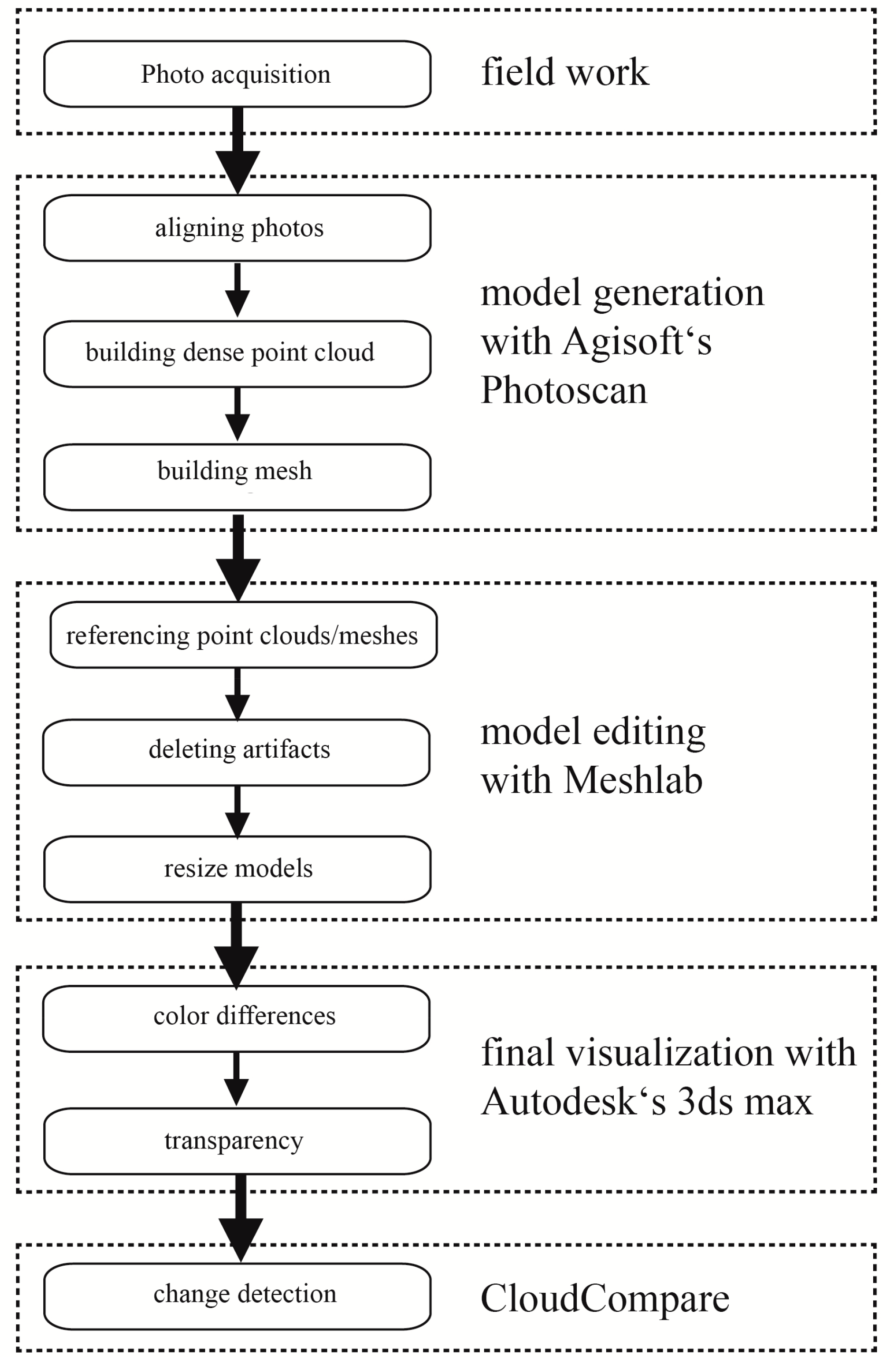
In a final step another software application was tested for capabilities in geomorphic data processing. CloudCompare [42] offers direct cloud-to-cloud or cloud-to-mesh distance measurements of major avail for the presented study as they offer a means to gain information on changes between two points in time or on a potential offset of the two methods. The software’s potential was of use in a way that distances between point clouds of two time steps could be measured and adequately visualized. In addition, the ability to convert different formats was convenient due to the amount of applied software. Furthermore, the straightforward referencing procedure of two time steps was applied to validate the accuracy of the foregone Meshlab-based referencing. Figure 5 sums up all the above software applications and gives an overview of the step-by-step workflow from image acquisition to the resulting models.
3.3.1. Calculation of Sediment Loss for the Moroccan Gullies
While calculating volumes of closed mesh objects or TINs is not a complex task in 3D data processing, eroded geomorphology usually consists of open and hollow landforms (i.e., gullies) which can be of high complexity. The difficulty with this kind of landform, such as rills, pits and gullies, is that the mesh needs to be a closed object to derive volume information. A solution is to fit a plain on top of the meshed model. Due to the complex edges of gullies, a perfect fit on high resolution surface data is hard to realize. Furthermore, only the active headcut areas were investigated. Both make a statement of absolute gully volumes difficult, though they enable information concerning volume of sediment loss for a certain period. For this approach, three-dimensional surface meshes need to be available from at least two different points in time. These meshes of the different dates of acquisition are referenced to each other either in MeshLab or CloudCompare by applying a rotation matrix Rωφκ (1) with the axes ω, φ, κ, after having identified rocks and boulders serving as GCPs surrounding the gullies on the models.
In a next step they are further processed in Autodesk’s 3Ds Max [43]: Firstly, the border of each model is punched out to have them covering the exact same area. For every mesh, a three-dimensional box is calculated from the model’s edge to a predefined value in elevation. This means that a box of known size is fitted below the reproduced land surface for each model. The volume is given by Autodesk 3ds Max. Any divergence from the result of x × y × z, equaling the volume of the artificial box fitted around the headcut can be attributed to the gully incision. Thus, differences in volume from box to box throughout the time steps are due to changes in the surface mesh, ultimately due to erosion or accumulation of sediment. For determining the soil loss, a total of 45 core samples were taken to acquire bulk density. Samples were mostly taken on the soil surface around the headcut, but also in sidewalls showing no significant variance.
3.3.2. Field Laboratory Experiments in Eichstätt—SfM vs. TLS
Besides the monitoring of natural rain events in Morocco, experiments under controlled conditions were carried out. Rainfall and rill flushing simulations were executed on bare and steep slopes in a quarry in Eichstätt, Germany. In addition to the simulated rainfall events, a tool to feed sediment-loaded runoff into the plot was installed to increase the virtual slope length [44]. Water amounts for the rill experiments varied between 30 and 120 L in a timespan from one to three minutes. Hereby, changes in surface morphology could be generated in a near-natural surrounding/setup. Images for the structure from motion application were taken before and after each experiment. Furthermore, the setup was supplemented with three video cameras from different angles for later analysis of the course of the experiments and possible occurrences of changes in the rill such a debris flow.
To allow later scaling to correct sizes, a variety of objects of known sizes was placed close to the surveyed form, which could be retrieved in the produced model, e.g., the plot boundary of a rainfall simulator [45]. In doing so, the time-consuming installation of GCPs and their calibration could be bypassed. This procedure was first applied in Morocco and is validated with LiDAR data in Eichstätt. As terrestrial laser scanning is commonly accepted as a useful tool for generating high resolution surface models with a high accuracy for geomorphological research [34–36], it served as an adequate tool for validation of the approach. For rill and rainfall experiments reflectors as GCPs were installed to co-register different LiDAR scans, but not the SfM models. All scan positions were chosen from slightly below the plot or rill on a plateau in front of the slope. To minimize shadowed areas behind minor elevations and thereby compensate the missing perspective from uphill, both positions were selected far from each other. In order to minimize the impact of differences in resolution, the point clouds produced with SfM were downscaled and resampled.
A total of three experiments were directly compared: two rainfall simulation plots and one rill experiment. Scans were performed from at least two different angles of each experimental site. For the validation of the motion-based image acquisition, a total of 333 images on all three sites were taken and processed. The comparably high number of images is a result of the rough and complex surface with many shadowed areas, e.g., behind upstanding stones. A number of 30 to 90 images per measured area of 1 m2 for the rainfall plots and 5 m2 for the rill experiment allows for a decent amount of perspectives to reduce these effects and increase detail in the output dataset.
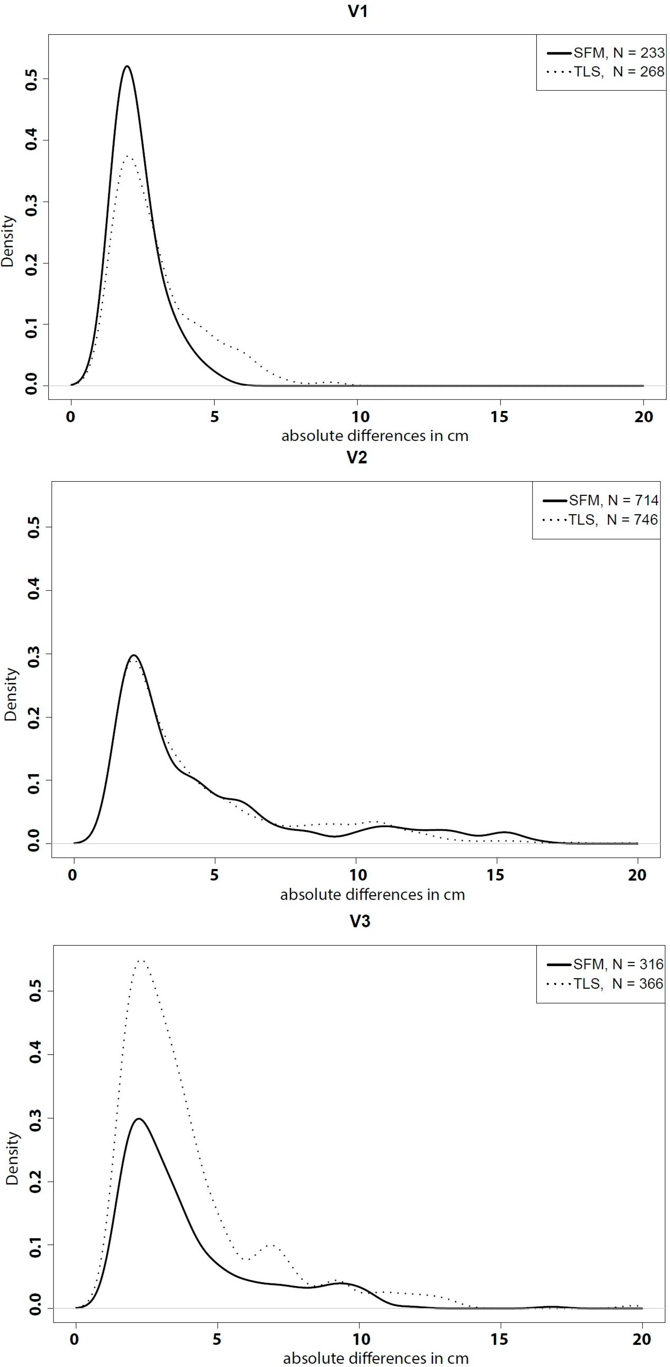
In order to validate the SfM-generated surface models, test plots were subject of data acquisition using SfM techniques and terrestrial LiDAR. For the SfM models as well as for the LiDAR scans, pre- and post-erosion surface models were referenced to each other. Point clouds from TLS and SfM were imported and binned into rasters with a cell size of 1 cm in LIS Desktop/SAGA GIS for further processing steps [12,37]. As a result two different raster datasets remained functioning as DEM of difference (DoD) for direct comparison: one for the SfM technique and one for terrestrial LiDAR. The aggregation of several points lying in one cell was done with mean values. Accumulation and erosion values were calculated from DoDs [39], where surface changes of <1 cm were treated as no surface change representing a low level of detection (LoD) value [32,39]. Because the datasets from the different acquisition techniques were not referenced to each other, the differences could not be compared for every grid cell but for the entire plot. By choosing the exact identical surface extents in both raster datasets, the difference in distributions of surface differences provide good information about the accuracy of the SfM surface models in comparison to the LiDAR models (Figure 6).
While the above-described accuracy assessment involves a rather classic grid-based approach, the following will explain a direct comparison between high resolution SfM meshes and TLS point clouds from the same point in time. Based on the statements by González-Aguilera et al. [46] about an accuracy assessment for a quarry site using UAV and TLS data, CloudCompare was applied to first manually reference the SfM mesh on the TLS point cloud which works as ground truth. In a second step, both models were clipped to give them a common edge and, accordingly, the same size. This was done along the plot border at the rainfall simulation site and close to the rill incision to compare only the areas of interest. After identifying appropriate GCPs, such as the plot border or prominent stones, mesh and point cloud are aligned. To enhance the accuracy of the registration, an ICP-algorithm is applied reducing the space between mesh and points [47]. For every point in the TLS point cloud, the distance to the meshed surface of the SfM model was calculated in order to measure existing distances between TLS surface and SfM mesh surface.
4. Results
4.1. Comparison between Laser Scans and Structure from Motion for the Test Site in Eichstätt
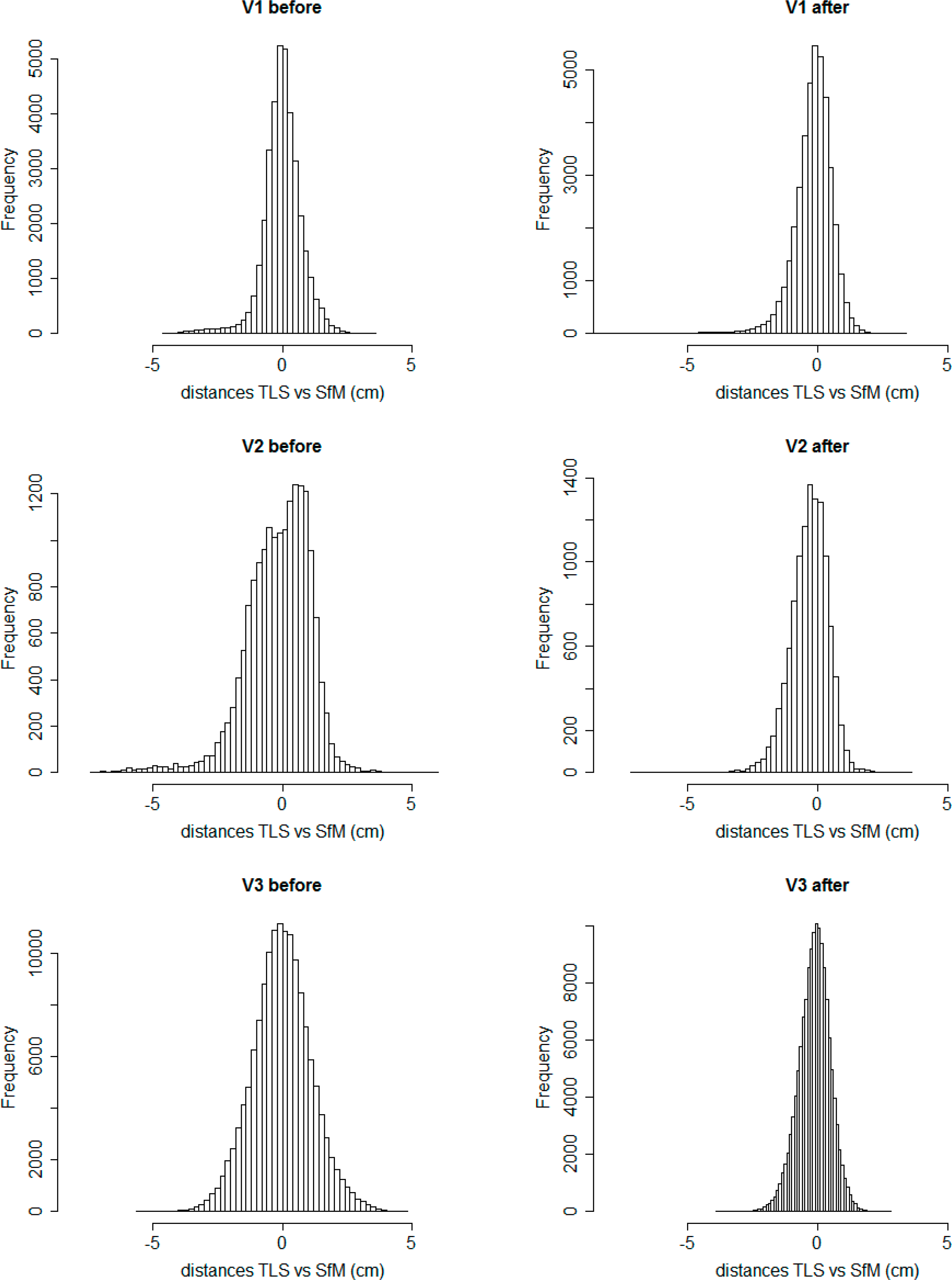
Figure 6 shows the residual distributions between pre- and post-erosion surface models for the different plots. On first sight, the TLS distributions are in good agreement with the SfM results (identical mode and standard deviation), thus pointing to the fact that the accuracy of SfM point clouds is comparable to LiDAR scans. Looking more into detail, however, only the test plot V1 shows noteworthy discrepancies between LiDAR and SfM. Whereas the maximum of the distribution is identical at around 2 cm for both techniques, the distributions differ slightly for values from 4 to 8 cm. Reasons for this shift can be of high variety, e.g., shadowing in the TLS data, or an undersampling of real topography by the TLS due to too great a point spacing. Despite these minor differences, the results strengthen the assumption that SfM data acquisition provides comparable results to terrestrial LiDAR scans and is therefore fully suitable for 3D erosion quantification and research. In addition to the residual distributions, total accumulation and erosion volumes of TLS and SfM grids correspond satisfyingly for each experiment. The differences are in the scope of several cm3 on small-scale plots designated for erosion research (Table 5). Mismatches between erosion and accumulation at each plot are the result of material that left the plot and thus the measured area downslope during the flushing simulations.
Table 6 demonstrates the differences acquired from a direct comparison between SfM and TLS data. The mean values between the models of both methods are in the scale of a few millimeters while the minimum and maximum do not exceed 8 cm in a few areas. Min values and values below zero represent areas where the referenced layer lies below the TLS model. After the ICP referencing, both models are intertwined. The total amounts of variations can be seen in histograms in Figure 7 also showing the highest discrepancies in both directions.
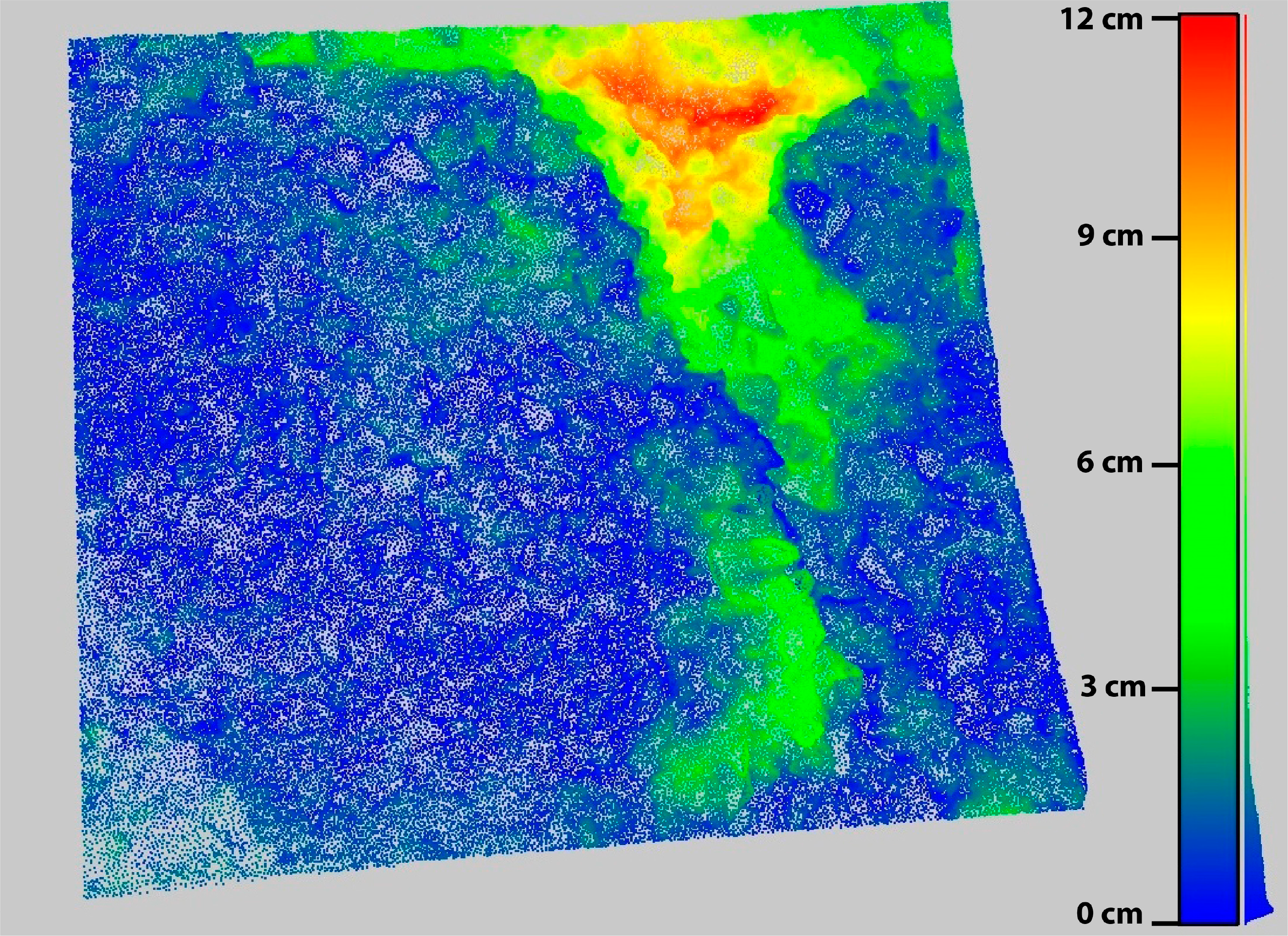
Results of the rainfall simulation in Eichstätt are visualized in Figure 8. The green region in the lower part of the figure represents positive discrepancies caused by the accumulation of eroded material. Its origin can be seen in the red source area of a small-scale debris flow initiated by adding runoff to the plot from above. Parts of the mass movement spilled over the plot boundary and thus left the model area, resulting in a negative sediment balance (Table 5).
4.2. Surface Models and Monitoring of the Gullies in Morocco
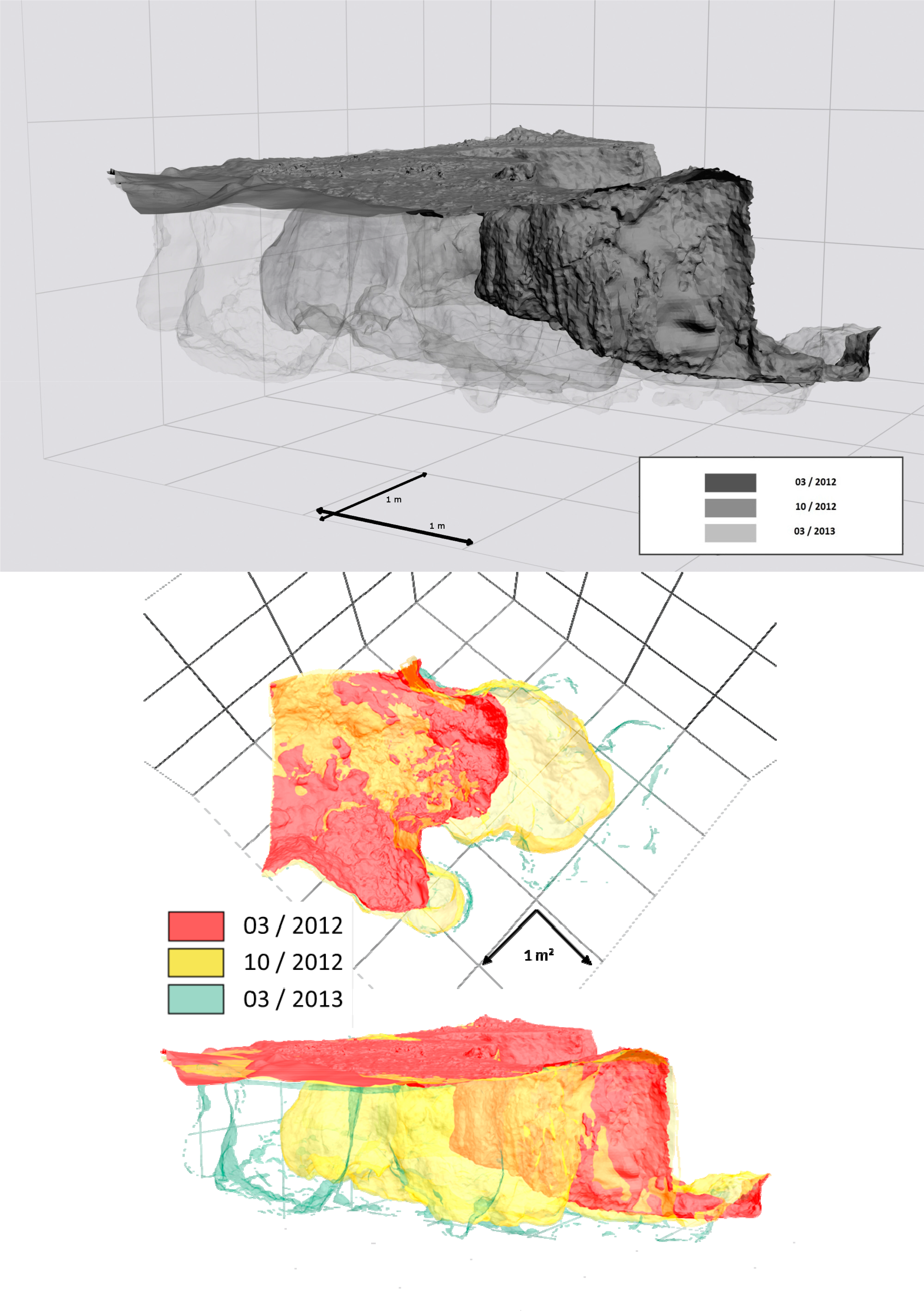
The following paragraph presents the results of measured soil loss volumes and models in different time steps (Figure 9 for the HAM gully, Figure 10 for GCH). Corresponding volume losses are given in Table 7. The obtained 1.5 g per cm3 (standard deviation of 0.12 g per cm3) was multiplied with the measured changes in volume. No absolute volume is given, as only headcut areas were analyzed with an artificial bounding box.
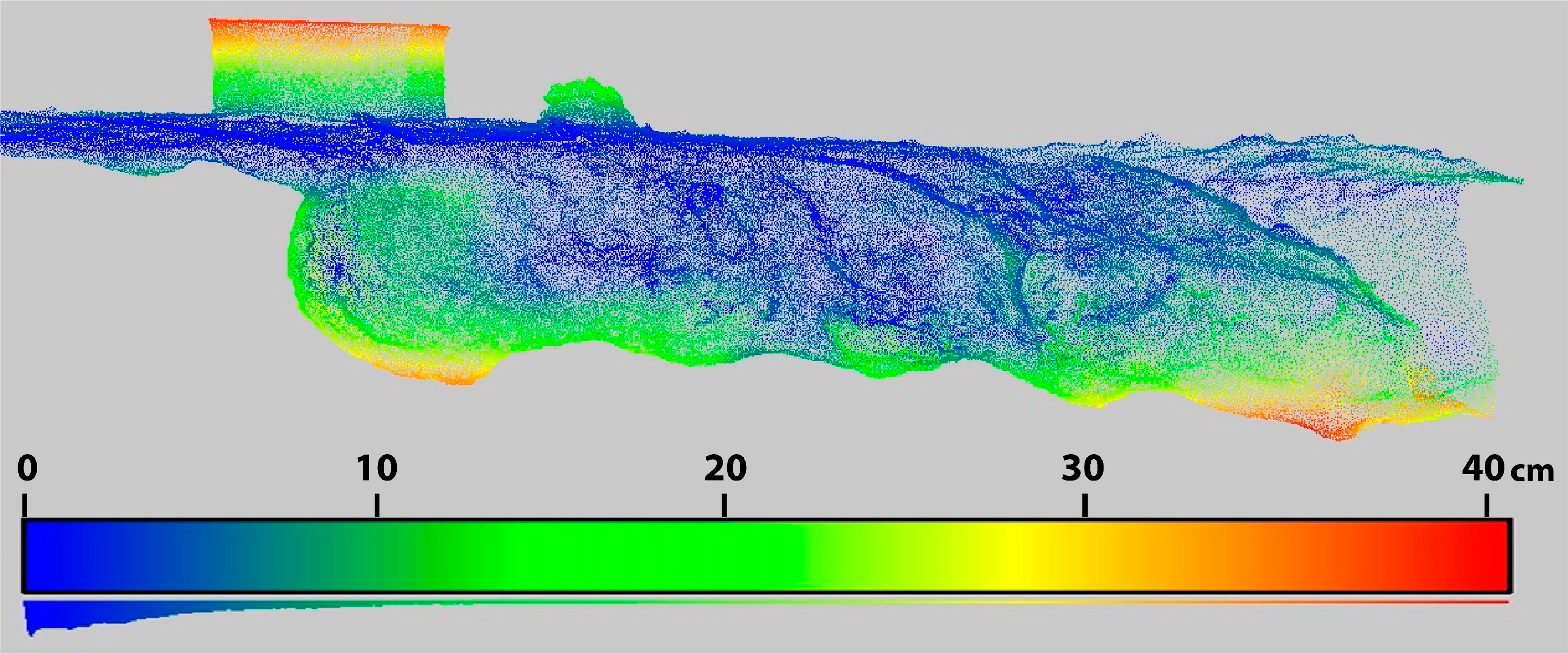
The following results show comparisons of two point clouds (.xyz), two meshes (.ply or .obj) and meshes and point clouds in CloudCompare [42]. Figure 11 depicts the research area HAM as a difference image. A histogram is calculated to show the distribution of variance between the two objects. The color scale on the right ranges from blue to red with blue representing small or no changes, while red indicates the biggest difference. Blue parts are predominant while red is restricted to the depression line and the plunge pool on the left. The scaling box (77 × 38 × 36 cm3) exhibits a red lid corresponding to its height of 38 cm. The biggest difference is seen in the lower part of the gully were maximum values of 42 cm of incision occurred. Also plant growth during the measuring period is evident which can be seen in the object right of the box.
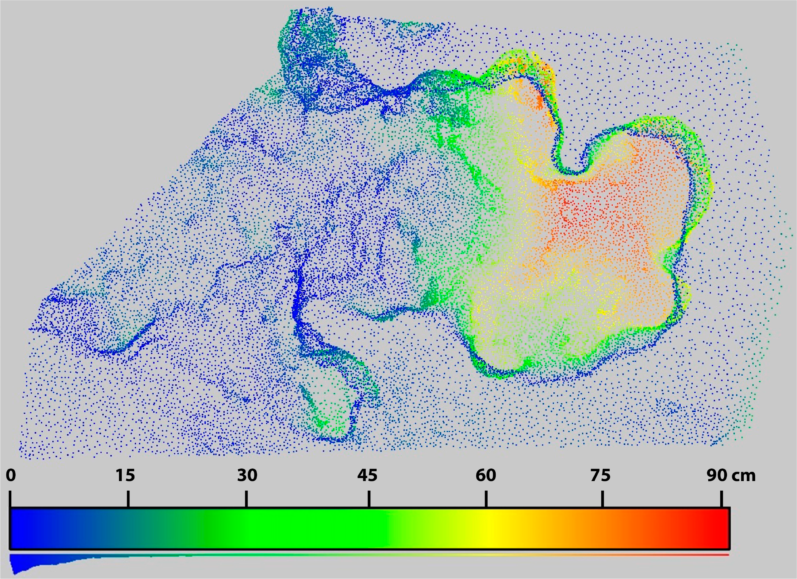
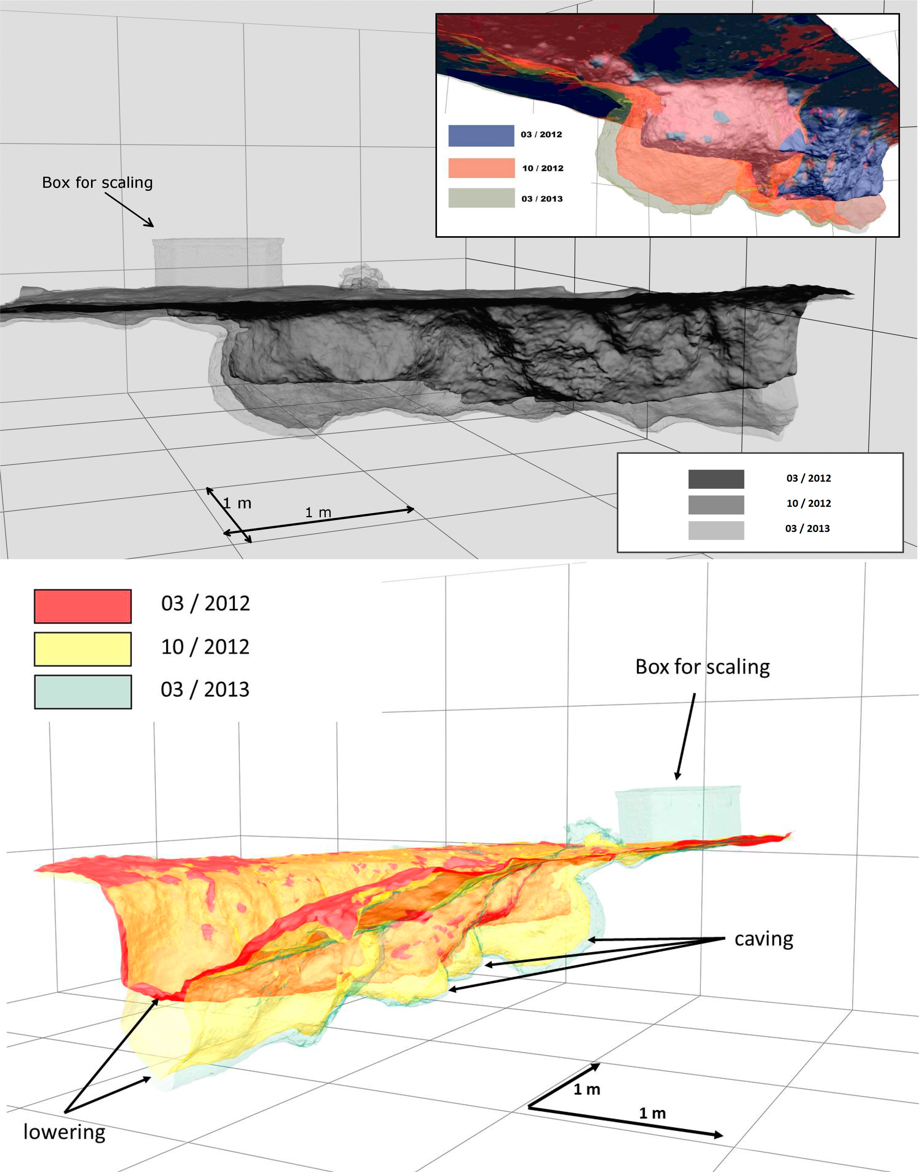
The GCH gully does not compare to the HAM site from the morphological point of view. Different processes form a surface without the presence of familiar erosion patterns. While the headcut retreated by almost 2 m, no clear rill incision is evident. A circular headcut retreat expands into the old land surface which is lowered to the level of the gully bottom. An incision caused by concentrated surface runoff cannot be detected. Figure 12 displays a high-angle shot of the expanse of the GCH gully between March 2012 and March 2013. The blue rim in the yellow part of the point cloud represents the new headcut. Partially, the hollow of the plunge pool expanded further than the headcut. Areas in front of the active incision remained more or less inactive as deposition of the washed-out material took place further downstream towards the wadi.
5. Discussion
Photogrammetric, laser and radar reconstruction techniques are steadily improving and the equipment becomes faster and smaller. A major improvement in this development is realized by the SfM approach and results underline positive findings with regard to accuracy and operability of SfM in other studies [9,17]. Especially in the understanding of geomorphological processes, the amount of model details allows new insights. The ability to measure hollow forms including undercuts and complex concavities in the headcut area of rills and gullies proves to be of major avail. Neglecting terrestrial approaches might lead to a continuous underestimation of gully volume as already described and when compared to aerial imagery [3]. Generalizing the gully cross-section as a trapezial shape with varying angles and surface areas is a useful approach for handling raster data for GIS software as long as the width of the gully bottom does not exceed the upper edge width [24]. Nevertheless, in order to precisely depict reality, raster data can hardly act as an appropriate tool. Field observations reveal numerous erosional shapes expanding under the current land surface which might soon trigger collapse of a gully sidewall. For airborne approaches, these invisible hollows can constitute large proportions of total soil loss (Figure 13). A variety of visualization methods was attempted (colorized, greyscale, mesh, wireframe, difference images from CloudCompare and different perspectives). Additionally, the implementation of north arrows and scale bar involve issues as the view angle would change length of the scale bar. Grids of 1 × 1 m were displayed behind the models to improve the impression of scale. For reasons of better visibility pictured as a blue wireframe, the undercut on the eroding bank of the gully HAM represent a suitable example for the advantages of SfM.
Furthermore, HAM serves as a model in order to increase knowledge about the interior hydraulics of a rill or a gully. Insights on the depression line and the interaction of slip-off slope and eroding bank are possible. The displayed incision illustrates a constant cutting into the substrate at a more or less 45° angle. This process is dependent on the erodibility of the material as a less erodible layer would cause lateral growth and reduce deepening [48].
Figure 14 demonstrates a possible final output of a SfM workflow. A meshed model of the HAM research site was overlain by textures derived from image data to create a photorealistic 3D impression.
In many cases, also hydrological models are dependent on surface models. On catchment scale, current raster data is sufficient [49]. However, flow simulation models such as HEC-RAS are able to reproduce channel and river flow dynamics and can benefit from high resolution surface models [50]. Not only in the gully head but also in the cut banks is soil eroded, causing sidewalls to collapse due to tension cracks under unsaturated conditions [51] and/or wall failure as a result of changes in potential energy [52]. All the above is made visible with a high degree of detail, even from below soil surface. In the example of HAM, an inactive headcut seen from bird’s eye view might lead to the misconception of an inactive gully system. The main reason for this is the partially correct assumption that gully growth occurs mainly at the upper end of the gully, denying the soil loss that actually leads to collapsing sidewalls and the further retreat. In HAM an unpaved trail used for land machines and pedestrians runs perpendicular to the direction of the gully incision, which causes the compacted soil to produce runoff rapidly while remaining stable in the upper few centimeters. Consequently, a growing plunge pool is currently faced by a resilient headcut (Figure 10).
In the GCH research area (Figures 10 and 12), a very gentle slope produces a wide and rather atypical form of gully. No clear rill incision is evident but a circular hollow form of 25 m in diameter and 1.5 m in depth developed. Besides the weak inclination of the terrain, Wells et al. (2013) [48] suggest another explanation contributing to the shape of GCH by connecting lower incision rates and thus widening to a less erodible soil layer. In rainfall simulations, measured sediment loads were low in comparison to other test sites in the research area, which can be explained by physical and biological soil crusts covering parts of GCH [24]. However, soil below crusts showed low aggregate stabilities in laboratory experiments applying the wet sieving method [53]. Hence, even small amounts of water inflow affected soil surface stability during a witnessed rain event in October (2012). Accordingly, soil detachment cannot be linked to discharge forces as high stream power triggered by high runoff velocities is non-existent. A reasonable explanation for GCH is chemical dispersion due to high sodicity as described by Levy et al. (2003) [54] and Amezketa et al. (2003) [55].
Throughout the study CloudCompare turned out to be a recommendable open source tool for point cloud and mesh processing [42]. It offers a variety of computational analysis for laser- or SfM-generated point clouds. Also triangular meshes can either be produced (Poisson reconstruction [33]) from point clouds or further processed. Referencing with GCPs and ICP, distance computation between two objects, general statistics and other processing algorithms are implemented. Another useful option is the conversion of many known 3D data file formats like .ply, .obj, .vtk and ASCII.
5.1. Time Requirements and Accuracy
Handling of 3D data usually is a time- and computing-capacity-consuming task. Image acquisition, though, is straightforward and took no more than 30 min for the presented gullies. Furthermore, it can be accelerated for larger areas by using a UAV covering multiple hectares in only one flight of 30 min, albeit with less detail than the terrestrial imagery if not combined with it. Data can also be derived as still images from a recorded movie of the respective surface. Experiments with a GoPro® camera on a headstrap, while walking inside a gully or attached to a handy and agile DJI® Phantom multicopter turned out to produce good quality models. Nevertheless, post-processing is still labor-intensive. While PhotoScan offers an easy workflow with an option for batch processing for bigger workloads, the additional steps described in the methodology are lengthy. Starting the batch in PhotoScan usually takes less than 15 min, depending on the amount of processed data. Each of the necessary working steps, starting with the import of the images, aligning the photos, building point clouds and meshes and ending with the saving of the project, has to be preset in the batch process. The then fully automatic calculating can exceed a few hours or even a night, again highly dependent on the amount of processed data. With an average computer system (Intel Pentium® i7 3770k, Nvidia® GeForce GTX 660 at 192-bit and 16GB DDR3 RAM), a high resolution model of 40 images takes around 90 min to process.
Concerning the accuracy, it is important to note that a classical accuracy assessment cannot and was not planned to be executed in the present study. The latter would require dGPS or tachymeter-measured GCPs that would allow for georeferencing the different methodologies. Studies describing the accuracy of SfM in different geomorphic contexts already exist [9,17,56,57], also for a larger-scale comparison of SfM vs. TLS [10]. Accuracies of the non-GCP approach are in a comparable extent as other studies, but depend on the scale of the respective object of interest. A small-scale approach like the 1 m2 plot in the presented work has not been published to the best of the authors’ knowledge. González-Aguilera et al. (2012), for example, present a standard deviation between 3.58 cm and 3.84 cm for SfM and TLS comparison in a large quarry in central Spain including GCPs [46]. Also, Westoby et al. (2012) compared SfM and TLS procedures in a geomorphological surrounding and presented frequency distributions, comparable to Figure 7, with similar characteristics [10]. However, both studies applied a GCP-based approach and tested a larger research area.
One main objective of the study was to develop a fast and practical way to derive volume data of lost soil without placing GCPs and register them with a tachymeter. Therefore, a possible solution for assessing the accuracy is the direct comparison of the residual distributions of DoDs derived for SfM and TLS models each. The applied gridding of the SfM and TLS point clouds seems contradictory to the above-recommended meshes for treating complex 3D morphology, but is suitable in the case of the rainfall plots and rills, as no visible undercuts were evident. Furthermore, grids have been an established tool in representing surface models and thus appear adequate for an accuracy assessment. Nevertheless, the additional accuracy assessment carried out in CloudCompare might be more representative for the present study, as it involved mesh and point cloud data and showed comparably good results. In this context, the influence of shadowing effects as a result of a restricted number of scan positions carries weight. While the mobile camera allows a huge number of different perspectives, the frequent relocation of the scanner is not feasible.
The highest Structure from Motion-based point counts of 57 million on a 1 m2 area shows the future development and possibilities of close-range photogrammetry. For available computing capacities, the 1.65 GB text file (xyz-coordinates) proved to be hardly manageable in post-processing. The amount of 5700 points/cm2 enables the visualization of grain sizes of the sand fraction (<2 mm). Depending on the applied lens, the theoretic Ground Sampling Distance (GSD) lies below 1 mm.
5.2. Application in Erosion Modelling
The presented SfM approach of avoiding GCP installation and registration and using objects for scaling allows for different applications in geosciences, especially in erosion research. In this field of research, soil erosion modelling is one beneficiary of the increasing computational capacities. Physical-based erosion models, such as EROSION 3D [58], WEPP [59] or LISEM [60], have been tested, improved and validated for decades and are capable of reproducing runoff-related erosion processes. As many erosion models are dependent on digital elevation models, their modelling abilities have mainly been used on large-scale land in agriculture. Here, raster cell sizes of 10 m × 10 m are sufficient for appropriately predicting erosion rates. With the ongoing development in high resolution surface modelling, the applicability of physical-based erosion models is possible on a higher detailed basis. Raster-based cellular automata are sensitive to cell sizes of the DEM which again can be influenced by the user’s choice. Short calculation time often results in a decision for a low resolution raster and thus changes in values derived from the DEM such as slope, the size of the watershed, and patterns in land cover [61]. As processing times are decreasing with the growing computer capacities [62], a trend towards more precision and small-scale erosion modelling is on the rise. In this context, the use of meshes or TINs offers new possibilities. The ability to handle several z-values above each other enables more dynamic modeling approaches as the natural behavior of runoff incision, rill formation and hydraulics can be depicted more precisely. Furthermore, the presented volume acquisition also applies for erosion modeling, as predicted soil loss volumes can be validated by SfM measurements, UAV based for large-scale agriculture, or terrestrial for event-based erosion damage like rill erosion or mud flows. The latter was realized with a DJI ® Phantom. Noteworthy is the fact that including slant photographs reduced the “bowl effect” of the resulting model. Not only in airborne images, but also terrestrial acquisition nadir pictures should be supplemented by slant frames.
6. Conclusions and Outlook
An advanced application of Structure from Motion algorithms in soil erosion monitoring was carried out in a Moroccan research area. Additionally, an accuracy assessment for the SfM method was peformed in Eichstätt, Germany. A non-ground control points approach was tested to avoid their tedious distribution and registration on two gully headcuts. Eroded volumes were quantified entirely by including undercuts and plunge pools into the meshed surface models. Results showed clear advantages over established approaches as shadowing effects were almost completely eliminated, new views of the gully interior became possible and a three-step surface change was visualized in 3Ds max. Soil losses reached from 0.58 t in the smaller gully headcut to 5.25 t in a larger one during the one-year monitoring campaign. The accuracy test of the non-ground control points approach comparing Structure from Motion meshes to terrestrial laser scanner point clouds showed good values between 0.61 cm and 1.26 cm standard deviation.
Nevertheless, further research is required to create a straightforward workflow. Besides the high workload for computers, 3D data is difficult in handling and requires experience by users during post-processing. While most parts of the workflow run automatically, there is still a high need for data conversion to different formats (.txt, .xyz, .ply, .obj), cutting of models, resampling, meshing and scaling. As a mature method, laser scanning data processing is easier and not as work intensive but more costly. An additional limitation that requires further thinking is how to properly visualize 3D data on a print such as the article at hand. Rotating, zooming and moving a 3D model offers infinite perspectives and conveys more information than the 2D print version. Tablet PCs and fast graphic processing units should be usable accordingly by scientific journals, also to promote visual process simulations. In a way forward and combined with emerging 3D printing technologies, the presented precise surface models offer interesting possibilities for experimental setups. A strong open source community is developing applications for Structure from Motion in order to rapidly implement improvements. Moreover, interdisciplinary applicability of the algorithms promotes novel interactions between sciences such as different physical sciences, informatics or engineering. A programming effort in Java 3D attained promising results in automated gully volume calculation but is yet to be tested with further data. As computer capacities are still growing, the presented work gives only an initial contribution to the field of high resolution surface reconstruction. The aim of approving the applicability of photography-based surface reconstruction in erosion research has been achieved. In combination with sufficient computing contingencies, SfM proves to be a useful tool and justifiably appears more often in the geomorphological community.
List of Abbreviations
| DEM | Digital Elevation Model |
| DoD | Digital Elevation Model of Difference |
| dGPS | differential Global Positioning System |
| GCP | Ground Control Point |
| GCH | Gschechda research site |
| GIS | Geographic Information System |
| GSD | Ground Sampling Distance |
| HAM | Hamar research site |
| HEC-RAS | Hydrologic Engineering Centers River Analysis System |
| ICP | Iterative Closest Point |
| LiDAR | Light Detection and Ranging |
| LISEM | Limburg Soil Erosion Model |
| LoD | Level of Detection |
| RGB | Red Green Blue color space |
| SfM | Structure from Motion |
| SIFT | Scale-Invariant Feature Transform |
| SFAP | Small-Format Aerial Photography |
| TLS | Terrestrial Laser Scanning |
| TOF | Time of Flight |
| TIN | Triangulated Irregular Network |
| UAV | Unmanned Airborne Vehicle |
| Wadi | English term for the Arabic word oued |
| WEPP | Water Erosion Prediction Project |
Acknowledgments
The above work was feasible due to the financial support of the German Research foundation (DFG; SCHM 1373/8-1, HA 5740/3-1, MA 2549/3). The authors would like to thank Hassan Ghafrani, Abdellatif Hanna, Daniel Peter, Jennifer Schimpchen, Jonas Tumbrink, Tobias Wilms and Bernt Hahnewald for the support during field work. Further thanks go to Vera Christ, Maximilian Strauch, Daniel Vivas Estevao, Robin Dinse for their still ongoing effort in compiling an automated gully volume calculation. The authors are also thankful for the quarry operator Georg Bergér GmbH to provide us with a field laboratory. We furthermore would like to thank all anonymous reviewers for their valuable recommendations which definitely improved the quality of the paper.
Author Contributions
Andreas Kaiser carried out the field work in three campaigns in Morocco and one in Eichstätt, collected the data, developed main parts of the workflow and produced and referenced SfM point clouds and meshes. Fabian Neugirg’s assignment was the terrestrial laserscanning. He took part in the Eichstätt field campaign, carried out all scans and their post processing, dealt with the statistics and their visualization and realized cloud to cloud measurements. Gilles Rock mainly worked on the final visualizations of the models in 3Ds Max and helped with the statistics. Additionally Andreas Kaiser, Fabian Neugirg and Gilles Rock were responsible for writing the manuscript. Christoph Müller joined one field campaign in Morocco to help with data acquisition and the soil samples. He helped with parts of the area description for the Souss Valley and accompanied the process of writing by repeated proof reading. Florian Haas helped with planning laser scanning campaigns, introduced the Eichstätt field laboratory and assisted during scan post processing. Furthermore, his criticism improved the overall quality of the paper. Johannes Ries chose all research sites in Morocco and joined two field campaigns. He led the project and critically accompanied the development of the method from the gully monitoring point of view. Jürgen Schmidt gave advice for the Eichstätt campaign, especially for the experimental setup during rainfall simulations. He repeatedly improved the manuscript by adjusting the order of paragraphs.
Conflicts of Interest
The authors declare no conflict of interest.
References
- Poesen, J. Challenges in gully erosion research. Landf. Anal 2011, 17, 5–9. [Google Scholar]
- Poesen, J.; Nachtergaele, J.; Verstraeten, G.; Valentin, C. Gully erosion and environmental change: Importance and research needs. Catena 2003, 50, 91–133. [Google Scholar]
- D’Oleire-Oltmanns, S.; Marzolff, I.; Peter, K.; Ries, J. Unmanned Aerial Vehicle (UAV) for monitoring soil erosion in morocco. Remote Sens 2012, 4, 3390–3416. [Google Scholar]
- Ries, J.B.; Marzolff, I. Monitoring of gully erosion in the Central Ebro Basin by large-scale aerial photography taken from a remotely controlled blimp. Catena 2003, 50, 309–328. [Google Scholar]
- Marzolff, I.; Poesen, J. The potential of 3D gully monitoring with GIS using high-resolution aerial photography and a digital photogrammetry system. Geomorphology 2009, 111, 48–60. [Google Scholar]
- Verhoeven, G.; Taelman, D.; Vermeulen, F. Computer Vision-based orthophoto mapping of complex archaological sites: The ancient quarry of Pitaranha. Archaeometry 2012, 54, 1114–1129. [Google Scholar]
- Farenzena, M.; Fusiello, A.; Gheradi, R. Efficient visualization of architectural models from a structure and motion pipeline. Proceedings of 29th Annual conference of the European Association for Computer Graphics (Eurographics’2008), Crete, Greece, 14–18 April 2008; pp. 235–238.
- Faugeras, O.D.; Lustman, F. Motion and structure from motion in a piecewise planar environment. Int. J. Patt. Recogn. Artif. Intell 1988, 2, 485–508. [Google Scholar]
- Castillo, C.; Pérez, R.; James, M.R.; Quinton, J.N.; Taguas, E.V.; Gómez, J.A. Comparing the accuracy of several field methods for measuring gully erosion. Soil Sci. Soc. Am. J 2012, 76, 1319. [Google Scholar]
- Westoby, M.J.; Brasington, J.; Glasser, N.F.; Hambrey, M.J.; Reynolds, J.M. “Structure-from-Motion” photogrammetry: A low-cost, effective tool for geoscience applications”. Geomorphology 2012, 179, 300–314. [Google Scholar]
- Turner, D.; Lucieer, A.; Watson, C. An automated technique for generating georectified mosaics from ultra-high resolution Unmanned Aerial Vehicle (UAV) Imagery, based on Structure from Motion (SfM) point clouds. Remote Sens 2012, 4, 1392–1410. [Google Scholar]
- Haas, F.; Heckmann, T.; Becht, M.; Cyffka, B. Ground-based laserscanning—A new method for measuring fluvial erosion on steep slopes. Proceedings of the Symposium JHS01, Melbourne, VIC, Australia, 28 June–7 July 2011; pp. 163–168.
- Höfle, B.; Griesbaum, L.; Forbriger, M. GIS-Based detection of gullies in terrestrial LiDAR data of the Cerro Llamoca Peatland (Peru). Remote Sens 2013, 5, 5851–5870. [Google Scholar]
- Liang, X.; Hyyppä, J.; Kaartinen, H.; Holopainen, M.; Melkas, T. Detecting changes in forest structure over time with bi-temporal terrestrial laser scanning data. ISPRS Int. J. Geo-Inf 2012, 1, 242–255. [Google Scholar]
- Marzolff, I.; Ries, J.B.; Poesen, J. Short-term versus medium-term monitoring for detecting gully-erosion variability in a mediterranean environment. Earth Surf. Process. Landf 2011, 36, 1604–1623. [Google Scholar]
- Wirtz, S.; Seeger, M.; Ries, J.B. Field experiments for understanding and quantification of rill erosion processes. Catena 2012, 91, 21–34. [Google Scholar]
- James, M.R.; Robson, S. Straightforward reconstruction of 3D surfaces and topography with a camera: Accuracy and geoscience application. J. Geophys. Res 2012, 117, 1–17. [Google Scholar]
- deCarta. Available online: www.decarta.com (accessed on 15 May 2014).
- Mensching. Marokko—Die Landschaften im Maghreb; Keysersche Verlagsbuchhandlung: Heidelberg, Germany, 1957. [Google Scholar]
- Burkhard, M.; Caritg, S.; Helg, U.; Robert-Charrue, C.; Soulaimani, A. Tectonics of the anti-atlas of Morocco. Compt. Rendus Geosci 2006, 338, 11–24. [Google Scholar]
- Aït Hssaine, A.; Bridgland, D. Pliocene–Quaternary fluvial and aeolian records in the Souss Basin, Southwest Morocco: A geomorphological model. Glob. Planet. Chang 2009, 68, 288–296. [Google Scholar]
- Food and Agriculture Organization. Carte Bioclimatique de la Zone Méditerranéenne (Notice Explicative)—Recherches sur la Zone Aride; Organisation des Nations Unies pour l’éducation, la science et la culture: Paris, France, 1963; Volume 21. [Google Scholar]
- El Ghannouchi, A. Dynamique Éolienne Dans la Plaine de Souss: Approche Modélisatrice de la lutte Contre l’Ensablement; Faculté des Sciences: Rabat, Morocco, 2007. [Google Scholar]
- Peter, K.D.; d’Oleire-Oltmanns, S.; Ries, J.B.; Marzolff, I.; Ait Hssaine, A. Soil erosion in gully catchments affected by land-levelling measures in the Souss Basin, Morocco, analysed by rainfall simulation and UAV remote sensing data. Catena 2014, 113, 24–40. [Google Scholar]
- Snavely, N.; Simon, I.; Goesele, M.; Szeliski, R.; Seitz, S.M. Scene Reconstruction and visualization from community photo collections. Proc. IEEE 2010, 98, 1370–1390. [Google Scholar]
- Ovod, D. Image capture tips—Equipment and shooting scenarios. Agisoft Photoscan Manual, Available online: http://www.agisoft.ru/tutorials/photoscan (accessed on 22 May 2014).
- Brown, D.C. Close-range camera calibration. Presented at Symposium on Close-Range Photogrammetry, Urbana, IL, USA, 26–29 January 1971; pp. 855–866.
- Fryer, J.G.; Brown, D.C. Lens distortion for close-range photogrammetry. Photogram. Eng. Remote Sens 1986, 52, 51–58. [Google Scholar]
- Agisoft. Lens. 2014. Available online: http://downloads.agisoft.ru/lens/doc/en/lens.pdf (accessed on 9 May 2014). [Google Scholar]
- Agisoft. PhotoScan. 2014. Available online: downloads.agisoft.ru/pdf/photoscan-pro_0_9_0_en.pdf (accessed on 12 May 2014). [Google Scholar]
- Lowe, D.G. Object recognition from local scale-invariant features. Proceedings of the International Conference of Computer Vision, Corfu, Greece, 20–25 September 1999.
- Brasington, J.; Rumsby, B.T.; McVey, R.A. Monitoring and modelling morphological change in a braided gravel-bed river using high resolution GPS-based survey. Earth Surf. Process. Landf 2000, 25, 973–990. [Google Scholar]
- Kazhdan, M.; Bolitho, M.; Hoppe, H. Poisson surface reconstruction. Proceedings of Annual Main Conference of the European Association for Computer Graphics (Eurographics 2006), Cagliari, Sardinia, 26–28 June 2006; pp. 61–70.
- Schürch, P.; Densmore, A.L.; Rosser, N.J.; Lim, M.; McArdell, B.W. Detection of surface change in complex topography using terrestrial laser scanning: Application to the Illgraben debris-flow channel. Earth Surf. Process. Landf 2011, 36, 1847–1859. [Google Scholar]
- Milan, D.J.; Heritage, G.; Hetherington, D. Application of a 3D laser scanner in the assessment of erosion and deposition volumes and channel change in a proglacial river. Earth Surf. Process. Landf 2007, 32, 1657–1674. [Google Scholar]
- Haas, F.; Heckmann, T.; Hilger, L.; Becht, M. Quantification and modelling of debris flows in the proglacial area of the Gepatschferner, Austria, using ground-based LiDAR. In Erosion and Sediment Yields in the Changing Environment; International Association of Hydrological Sciences: Oxfordshire, UK, 2012; pp. 293–302. [Google Scholar]
- Rieg, L.; Wichmann, V.; Rutzinger, M.; Sailer, R.; Geist, T.; Stötter, J. Data infrastructure for multitemporal airborne LiDAR point cloud analysis—Examples from physical geography in high mountain environments. Comput. Environ. Urban Syst 2014, 45, 137–146. [Google Scholar]
- Riegl, J.; Studnicka, N.; Ullrich, A. Merging and processing of laser scan data and high-resolution digital images acquired with a hybrid 3D laser sensor. Proceedings of XIX CIPA Symposium, Antalya, Turkey, 30 September–4 October 2003.
- Wheaton, J.M.; Brasington, J.; Darby, S.E.; Sear, D.A. Accounting for uncertainty in DEMs from repeat topographic surveys: Improved sediment budgets. Earth Surf. Process. Landf 2009, 35, 136–156. [Google Scholar]
- Charlton, M.E.; Coveney, S.; McCarthy, T. Issues in laser scanning. In Laser Scanning for the Environmental Sciences; Wiley-Blackwell: Chichester, UK, 2009; pp. 35–48. [Google Scholar]
- Lichti, D.; Skaloud, J. Registration and calibration. In Airborne and Terrestrial Laser Scanning; Vosselman, G., Maas, H.-G., Eds.; Whittles Publishing: Dunbeath, UK, 2010. [Google Scholar]
- Girardeau-Montaut, D. CloudCompare (Version 2.4) (GPL Software); EDF R&D, Telecom Paris Tech: Paris, France, 2014; Available online: http://www.danielgm.net/cc/ (accessed on 12 February 2014). [Google Scholar]
- Autodesk. 3Ds Max. 2014. Available online: http://store.autodesk.eu/store/adsk/en_IE/DisplayHomePage (accessed on 7 June 2014). [Google Scholar]
- Schindewolf, M. Parameterization of the EROSION 2D/3D soil erosion model using a small-scale rainfall simulator and upstream runoff simulation. Catena 2012, 91, 47–55. [Google Scholar]
- Michael, A. Anwendung des Physikalisch Begründeten Erosionsprognosemodells EROSION 2D/3D—Empirische Ansätze zur Ableitung der Modellparameter. Ph.D. Dissertation. University of Freiberg, Freiberg, Germany, 2000. [Google Scholar]
- González-Aguilera, D.; Fernández-Hernández, J.; Mancera-Taboada, J.; Rodriguez-Gonzálvez, P.; Hernández-López, D.; Felipe-García, B.; Gozalo-Sanz, I.; Arias-Perez, B. 3D modelling and accuracy assessment of Granite Quarry using unmanned aerial vehicle. ISPRS Ann. Photogram. Remote Sens. Spat. Inf. Sci 2012, 1, 37–42. [Google Scholar]
- Besl, P.J.; McKay, N.D. A method for registration of 3-D shapes. IEEE Trans. Pattern Anal. Mach. Intell 1992, 14, 239–256. [Google Scholar]
- Wells, R.R.; Momm, H.G.; Rigby, J.R.; Bennett, S.J.; Bingner, R.L.; Dabney, S.M. An empirical investigation of gully widening rates in upland concentrated flows. Catena 2013, 101, 114–121. [Google Scholar]
- Hümann, M.; Schüler, G.; Müller, C.; Schneider, R.; Johst, M.; Caspari, T. Identification of runoff processes—The impact of different forest types and soil properties on runoff formation and floods. J. Hydrol 2011, 409, 637–649. [Google Scholar]
- Hydrologic Engineering Center. U.S. Army Corps of Engineers. In HEC-GeoRAS—An Application for Support of HEC-RAS Using ARC/INFO—User’s Manual; US Army Corps of Engineers, USGS: Reston, VA., USA, 2005. [Google Scholar]
- Martinez-Casanovas, J.A.; Ramos, M.C.; Poesen, J. Assessment of sidewall erosion in large gullies using multi-temporal DEMs and logistic regression analysis. Geomorphology 2004, 58, 305–321. [Google Scholar]
- Collison, A.J.C. The cycle of instability: Stress release and fissure flow as controls on gully head retreat. Hydrol. Process 2001, 15, 3–12. [Google Scholar]
- Kemper, W.D.; Rosenau, R.C. Methods of soil analysis. In Aggregate Stability and Size Distribution; American Society of Agronomy: Madison, WI, USA, Soil Science Society of America: Madison, WI, USA; 1986; pp. 425–442. [Google Scholar]
- Levy, G.J.; Mamedov, A.I.; Goldstein, D. Sodicity and water quality effects on slaking of aggregates from semi-arid soils. Soil Sci 2003, 168, 552–562. [Google Scholar]
- Amezketa, E.; Aragués, R.; Carranza, R.; Urgel, B. Chemical, spontaneous and mechanical dispersion of clays in arid-zone soils. Span. J. Agric. Res 2003, 2003, 95–107. [Google Scholar]
- Javernick, L.; Brasington, J.; Caruso, B. Modeling the topography of shallow braided rivers using Structure-from-Motion photogrammetry. Geomorphology 2014, 213, 166–182. [Google Scholar]
- Verhoeven, G.; Doneus, M.; Briese, C.; Vermeulen, F. Mapping by matching: A computer vision-based approach to fast and accurate georeferencing of archaeological aerial photographs. J. Arch. Sci 2012, 39, 2060–2070. [Google Scholar]
- Schmidt, J. A mathematical model to simulate rainfall erosion. In Erosion, Transport and Deposition Processes—Theories and Models; Elsevier: Amsterdam, The Netherlands, 1991; Catena Supplement; pp. 101–109. [Google Scholar]
- Nearing, M.A.; Foster, G.R.; Lane, L.J.; Finker, S.C. A process-based soil erosion model for USDA-water erosion prediction project technology. Am. Soc. Agric. Eng 1989, 32, 1587–1593. [Google Scholar]
- De Roo, A.P.J.; Wesseling, C.G. LISEM: A single-event physically based hydrological and soil erosion model for drainage basins. I.: Theory, input and output. Hydrol. Process 1996, 8, 1107–1117. [Google Scholar]
- Jetten, V.; Govers, G.; Hessel, R. Erosion models: Quality of spatial predictions. Hydrol. Process 2003, 17, 887–900. [Google Scholar]
- Moore, G.E. Cramming more components onto integrated circuits. Proc. IEEE 1998, 86, 82–85. [Google Scholar]


| Coefficient | Distortion Values |
|---|---|
| K1 | −0.160095 |
| K2 | 0.14829 |
| K3 | −0.121853 |
| P1 | −0.00210068 |
| P2 | 5.4896 × 10⁵ |
| Model Label | Number of Images | Face Count | Vertices | Model Area (m2) |
|---|---|---|---|---|
| HAM 03/2012 | 247 | 17,251,912 | 8,630,314 | 18.65 |
| HAM 10/2012 | 388 | 24,455,149 | 12,231,631 | 18.65 |
| HAM 03/2013 | 178 | 35,087,777 | 17,551,504 | 18.65 |
| GCH 03/2012 | 560 | 29,161,542 | 14,587,625 | 17.45 |
| GCH 10/2012 | 104 | 19,451,856 | 9,596,328 | 17.45 |
| GCH 03/2013 | 108 | 21,729,454 | 10,865,195 | 17.45 |
| V1 before | 35 | 681,072 | 343,628 | 1 |
| V1 after | 30 | 512,974 | 259,792 | 1 |
| V2 before | 62 | 604,979 | 307,104 | 1 |
| V2 after | 91 | 1,147,046 | 580,208 | 1 |
| V3 before | 69 | 1,084,124 | 548,801 | 2.85 |
| V3 after | 46 | 702,978 | 354,866 | 2.85 |
| TLS Parameters | Riegl LMS-Z420i Values |
|---|---|
| max. measurement range | 1000 m for objects with a reflectivity value of ≥80% 350 m for objects with a reflectivity value of ≥10% |
| distance accuracy | 10 mm for a range of 50 m under test conditions |
| scanning rate | 8000 points per second |
| laser wavelength | near infrared |
| beam divergence | 0.25 mrad |
| increase of footprint (beam width) for vertical striking | 0.0025 m/100 m |
| Experiment | Range TLS-Plot | Average Slope of Plot | Horizontal Point Spacing | Footprint Short Axis | Vertical Point Spacing | Footprint Long Axis |
|---|---|---|---|---|---|---|
| V1 | 16.5 m | 70° | 5.7 mm | 4.1 mm | 6.1 mm | 4.4 mm |
| V2 | 20.4 m | 70° | 7.1 mm | 5.1 mm | 7.6 mm | 5.5 mm |
| V3 | 6.3 m | 45° | 2.2 mm | 1.6 mm | 3.1 mm | 2.3 mm |
| Experiment | Erosion TLS (cm3) | Sedimentation TLS (cm3) | Erosion SfM (cm3) | Sedimentation SfM (cm3) | Erosion Difference TLS-SfM (cm3) | Sediment Difference TLS-SfM (cm3) |
|---|---|---|---|---|---|---|
| V1 | −1528.5 | 596.4 | −1496.2 | 644.0 | −32.3 | −47.6 |
| V2 | −9833.8 | 3464.9 | −10,155.5 | 3060.3 | 321.7 | 404.6 |
| V3 | −5521.2 | 262.8 | −4340.1 | 548.2 | −1181.1 | 285.4 |
| Model Label | Mean (cm) | Min (cm) | Max (cm) | SD (cm) | RMSE Registration (cm) |
|---|---|---|---|---|---|
| V1 before | −0.01 | −4.44 | 3.43 | 0.77 | 0.91 |
| V1 after | −0.18 | −8.72 | 3.28 | 0.79 | 0.74 |
| V2 before | −0.16 | −7.22 | 5.91 | 1.26 | 1.41 |
| V2 after | −0.32 | −7.04 | 3.42 | 0.72 | 0.79 |
| V3 before | −0.01 | −5.54 | 4.77 | 1.14 | 0.92 |
| V3 after | −0.13 | −3.81 | 2.74 | 0.61 | 0.73 |
| Timespan | GCH | HAM | |||||
|---|---|---|---|---|---|---|---|
| Change (m3) | Soil Loss (t) | Headcut Retreat (m) | Change (m3) | Soil Loss (t) | Headcut Retreat (m) | Plunge Pool Drop (m) | |
| 03/2012 → 10/2012 | 1.94 | 2.91 | 1.11 | 0.21 | 0.32 | 0.04 | 0.37 |
| 10/2012 → 03/2013 | 1.56 | 2.34 | 0.84 | 0.17 | 0.26 | - | 0.05 |
| total | 3.5 | 5.25 | 1.95 | 0.38 | 0.58 | 0.04 | 0.42 |
© 2014 by the authors; licensee MDPI, Basel, Switzerland This article is an open access article distributed under the terms and conditions of the Creative Commons Attribution license (http://creativecommons.org/licenses/by/3.0/).
Share and Cite
Kaiser, A.; Neugirg, F.; Rock, G.; Müller, C.; Haas, F.; Ries, J.; Schmidt, J. Small-Scale Surface Reconstruction and Volume Calculation of Soil Erosion in Complex Moroccan Gully Morphology Using Structure from Motion. Remote Sens. 2014, 6, 7050-7080. https://doi.org/10.3390/rs6087050
Kaiser A, Neugirg F, Rock G, Müller C, Haas F, Ries J, Schmidt J. Small-Scale Surface Reconstruction and Volume Calculation of Soil Erosion in Complex Moroccan Gully Morphology Using Structure from Motion. Remote Sensing. 2014; 6(8):7050-7080. https://doi.org/10.3390/rs6087050
Chicago/Turabian StyleKaiser, Andreas, Fabian Neugirg, Gilles Rock, Christoph Müller, Florian Haas, Johannes Ries, and Jürgen Schmidt. 2014. "Small-Scale Surface Reconstruction and Volume Calculation of Soil Erosion in Complex Moroccan Gully Morphology Using Structure from Motion" Remote Sensing 6, no. 8: 7050-7080. https://doi.org/10.3390/rs6087050
APA StyleKaiser, A., Neugirg, F., Rock, G., Müller, C., Haas, F., Ries, J., & Schmidt, J. (2014). Small-Scale Surface Reconstruction and Volume Calculation of Soil Erosion in Complex Moroccan Gully Morphology Using Structure from Motion. Remote Sensing, 6(8), 7050-7080. https://doi.org/10.3390/rs6087050