Decision Fusion Based on Hyperspectral and Multispectral Satellite Imagery for Accurate Forest Species Mapping


Abstract
: This study investigates the effectiveness of combining multispectral very high resolution (VHR) and hyperspectral satellite imagery through a decision fusion approach, for accurate forest species mapping. Initially, two fuzzy classifications are conducted, one for each satellite image, using a fuzzy output support vector machine (SVM). The classification result from the hyperspectral image is then resampled to the multispectral’s spatial resolution and the two sources are combined using a simple yet efficient fusion operator. Thus, the complementary information provided from the two sources is effectively exploited, without having to resort to computationally demanding and time-consuming typical data fusion or vector stacking approaches. The effectiveness of the proposed methodology is validated in a complex Mediterranean forest landscape, comprising spectrally similar and spatially intermingled species. The decision fusion scheme resulted in an accuracy increase of 8% compared to the classification using only the multispectral imagery, whereas the increase was even higher compared to the classification using only the hyperspectral satellite image. Perhaps most importantly, its accuracy was significantly higher than alternative multisource fusion approaches, although the latter are characterized by much higher computation, storage, and time requirements.
1. Introduction
Designing efficient forest preservation and management policies requires the detailed knowledge of the species composition and distribution over large forested areas. However, the assessment of tree species distribution through ground-level field surveys is a difficult, expensive, and time-consuming task. The rapidly evolving remote sensing technology can greatly assist such studies, providing a means for automatic or (most frequently) semi-automatic characterization of large areas with limited user interaction.
The continuous advent of remote sensing sensors accommodate the even faster and more accurate mapping of various forest species. Very high resolution (VHR) remotely sensed imagery like QuickBird, IKONOS, and SPOT5 have proven valuable in discriminating various forest species over older generation sensors [1,2], as they can accurately describe the complex spatial patterns typically observed in forested areas. Moreover, a number of recent studies have shown that hyperspectral imagery are particularly useful for discriminating different species of the same genus, which is not always possible using the limited spectral information provided by VHR multispectral images [3–8]. The findings of these studies suggest that the dense sampling of the spectral signature provided by hyperspectral sensors is a precondition for accurate discrimination of similar forest species.
The high number of remote sensing sensors available today, as well as the possibility to acquire images of the same area by different sensors, has resulted in scientific research focusing on fusing multi-sensor information as a means of combining the comparative advantages of each sensor. Fusion is a broad term covering many different approaches, which in the field of remote sensing is most frequently employed to describe data fusion, that is, combination on the feature space level. A common form of multispectral/hyperspectral data fusion relates to resampling techniques, similar to pan-sharpening methods employed on multispectral imagery, a research field blooming in recent years [9–11].
Another form of data fusion frequently proposed is the so-called vector stacking approach (also known as image stacking), which produces a composite feature space by aggregating the input vectors from multiple sources and subsequently performs the classification on the new feature space. An important recent application of this approach has been the combination of multispectral or hyperspectral data with radar (SAR) [12,13] or—most commonly—with LiDAR [6,14–17] information. Other studies use a single source of primary information, which is then fused with new textural features derived from the initial image [18,19] or features obtained through object-based image analysis [20,21].
An alternative approach to data fusion is to employ the fusion process on the decision level, that is, to perform multiple independent classifications and then combine the output of the classifiers. A common application of decision fusion in remote sensing relates with the derivation of some form of textural features from a single source, the creation of an independent classifier for each source, and the subsequent combination of their outputs, following a divide-and-conquer approach. This approach has been successfully employed to combine spectral information with various families of textural features [22], morphological profiles [23,24], and image segmentation derived features [20,21]. In these studies fusion is performed on the classifiers’ soft outputs (either probabilistic or fuzzy), through simple weighted averaging schemes [20,21,24], more complex fusion operators [22], or even by considering the stacked (soft) outputs of the multiple classifiers as a new feature space and subsequently training a new classifier on this new space [23]. Decision fusion has also been exploited for effectively tackling the very high dimensionality of hyperspectral data, by training multiple classifiers on different feature subsets derived from the source image and then combining their outputs [25–29]. The feature subsets are derived either through some appropriate feature extraction algorithm [25] or—more commonly—by applying some feature subgroups selection process [26–29]. A more direct decision fusion approach combines the outputs of multiple different classifiers applied to a common data source [30–32].
Regarding the simultaneous evaluation of multi-sensor data, decision fusion has been previously proposed for combining multispectral data with geographical information (slope, elevation, etc.) [33–35]. In these studies, the information from multiple sources is combined through a so-called consensus rule, which fuses the outputs of multiple maximum likelihood (ML) classifiers, each trained on a separate data source. Benediktsson and Kanellopoulos [36] expanded this idea by considering a neural network (NN) classifier simultaneously with the consensus-theoretic ML classifiers. When the two classifiers disagreed, the decision was taken by a third NN classifier, which had been trained independently from the other two classifiers. Both NNs were trained on the aggregate feature space, created by stacking all individual data sources into a single vector. Waske and Benediktsson [37] presented a scheme for fusing a multispectral image with multi-temporal SAR data. The latter are first resampled to the multispectral image’s spatial resolution. Subsequently, an SVM classifier is created for each one of the data sources, their soft outputs are fused, and a separate SVM is trained on the fused output, in order to perform the final classification. This approach was extended in [38], considering additional SVM classifiers, trained on features derived from multi-scale segmentations. Finally, decision fusion has been exploited for combining multi-temporal satellite data [12,39,40]. However, these studies apply the fusing operator in order to combine the results at different time points, thus producing class transition maps. When multi-sensor data are considered [12,40], a typical vector stacking is followed.
All the aforementioned multi-sensor fusion approaches have a common disadvantage: the multisource information has to be registered into a single (spatial) resolution, typically the highest available one. Only the fusing scheme presented in [39] does not require the various images to be co-registered, but this approach relates to multi-temporal class transition estimation and cannot be applied to multi-source land cover classification. Down-sampling satellite imagery—especially hyperspectral ones—involves high computational demands and storage requirements. Even with modern computer systems, handling such high volume of data becomes at least cumbersome. For all data fusion approaches, co-registering the multiple data sources into a common spatial resolution is unavoidable. On the other hand, the decision fusion approach offers the possibility of performing the independent (that is, one for each data source) classifications in their native resolution, if an appropriate formulation is considered. Although the multiple classification maps still have to be co-registered to the finer spatial resolution, the computational burden and data volume produced is orders of magnitude less than resampling a hyperspectral imagery with hundreds of bands into the resolution of a VHR multispectral imagery.
Under this rationale, the current study investigates the effectiveness of a decision fusion scheme, aiming at combining the information provided by a VHR multispectral and a medium spatial resolution hyperspectral image. The proposed methodology constructs two independent fuzzy output classifiers using only the original bands of the two images, which are then combined by a soft fusion operator. To the best of our knowledge, no similar approach has been previously proposed for the direct combination of multispectral and hyperspectral data on the decision level. The specific objectives of the study are:
To validate the effectiveness of the new methodology on a complex Mediterranean forest mosaic in northern Greece.
To compare its performance with the commonly applied data fusion alternatives.
To investigate the potentials specifically of satellite hyperspectral imagery—which is typically characterized by medium spatial resolution—within the proposed fusion framework.
Regarding the last objective, we should note that the methodology is general and not restricted by the specific source considered. Admittedly, the vast majority of hyperspectral imagery studied in the respective remote sensing data fusion literature is acquired through airborne sensors. However, the cost involved with the sensor acquisition and the subsequent flight programming is usually very high, especially when larger areas need to be characterized. Presently, Hyperion [41] is the only spaceborne hyperspectral sensor, which was based on a very important but currently expired pilot mission. Nevertheless, a number of new missions designed to provide high quality hyperspectral satellite products have been programed for the near future, including EnMap [42], PRISMA [43], and HyspIRI [44]. To this end, the current proposal aims at proving a fast and reliable means for accurate forest species mapping in the foreseeable future, when new on-demand satellite hyperspectral products become available.
2. Materials and Methods
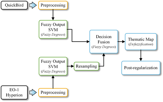
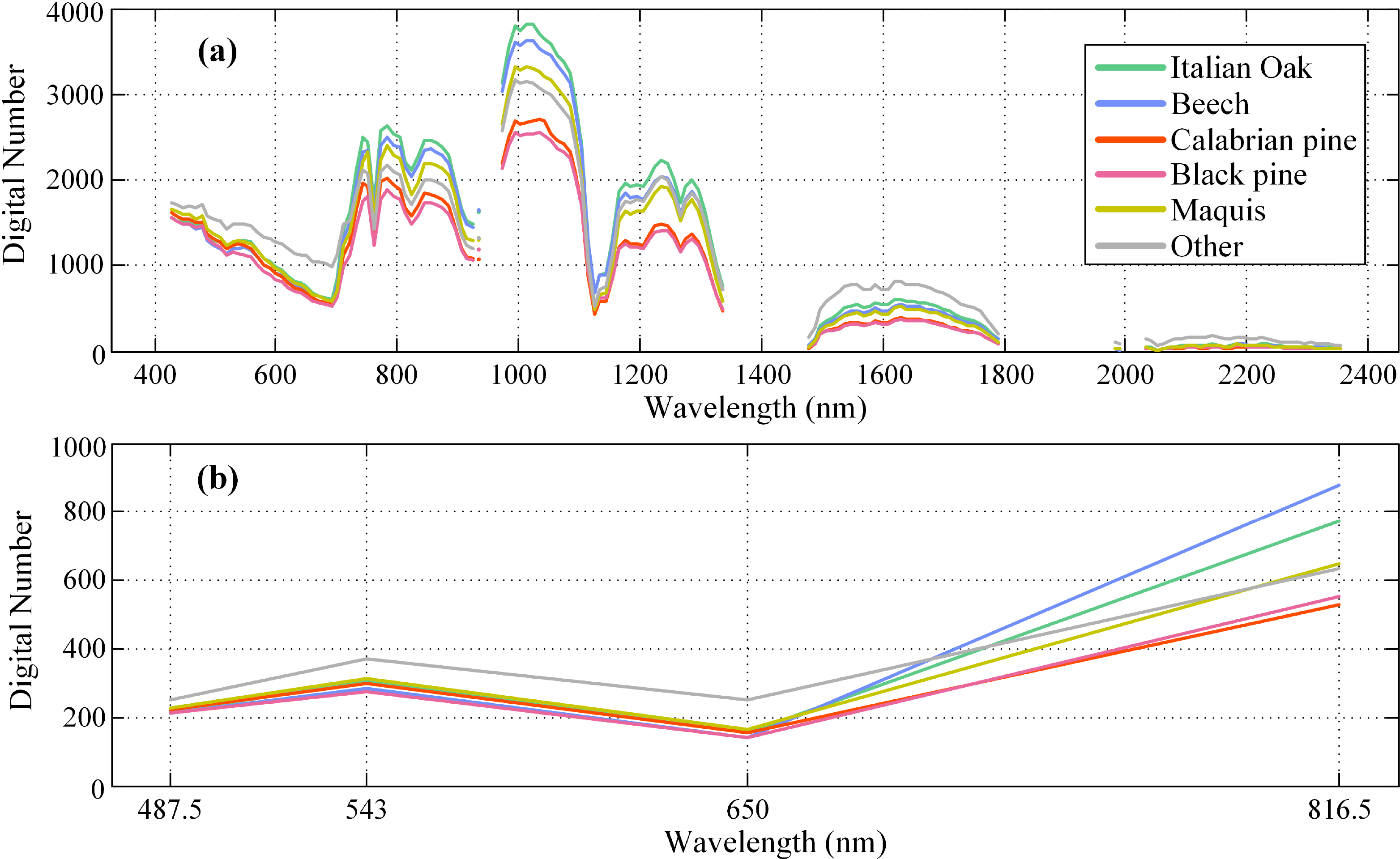
The present study investigates the effectiveness of combining a high spatial resolution multispectral satellite image with a hyperspectral one on the classifier’s decision level. An outline of the proposed methodology is depicted in Figure 1. We used a QuickBird multispectral image and an EO-1 Hyperion hyperspectral image over the same Mediterranean site in northern Greece. At the present time, Hyperion is the only spaceborne hyperspectral instrument to acquire both visible near-infrared (400–1000 nm) and shortwave infrared (900–2500 nm) spectra [41].
After preprocessing, the two images were separately classified using the support vector machines (SVM) classifier. SVM is a complex distribution-free classifier, based on a robust theoretical framework [45]. Its use was adopted in this study due to the high classification accuracy it has demonstrated in many remote sensing applications the past few years [46] and, particularly, in the classification of hyperspectral data [47–49]. We actually used a modified version of the original SVM, which is capable of producing a continuous output (that is, a fuzzy degree in the range [0,1] for each class), along with the crisp classification decision.
The application of the fuzzy output SVM on each image produces two fuzzy thematic maps. Hyperion’s map is resampled to match QuickBird’s spatial resolution. The two maps are subsequently combined using a decision fusion operator and the crisp classification decision is derived through a defuzzification process. The final thematic map is further post-processed through a simple algorithm that removes the noise (salt-and-pepper effect) to a considerable degree. The rest of this section details the datasets used and the various parts of the methodology.
2.1. Study Area
The University Forest of Taxiarchis is located on the southern and southwestern slopes of Mount Cholomontas in Chalkidiki, in the Central Macedonia region. It extends from 40°23′E to 40°28′E and 23°28′N to 23°34′N and covers an area of 60 km2 (Figure 2). The University Forest area is also part of the NATURA2000 network (GR1270001-Oros Cholomontas). The terrain of the study area is diverse and very rough at places as a result of high difference in altitude, ranging between 320 and 1200 m. The Mediterranean climate of the area is characterized by short periods of drought, hot summers and mild winters. Main characteristic of the climate is the large fluctuations of rainfall during summer as well as the double dry season (July and September) with limited duration and intensity [50].
The study area forms a complex mosaic. Common forest species are Italian oak (Quercus frainetto), Calabrian pine (Pinus brutia), Black pine (Pinus nigra), Beech (Fagus sylvatica), and Norway spruce (Pice abies). Gradually mixed stands have formed, as deciduous species invade the areas occupied by pines. In addition, patches within the forest are covered with maquis (Quercus ilex, Quercus coccifera, Erica arborea, etc.), low herbaceous vegetation and scattered oak trees [51].
2.2. Satellite Imagery
As mentioned previously, imagery from two spaceborne sensors was used in this study, namely, a QuickBird multispectral satellite image and a Hyperion hyperspectral one (Figure 3).
The QuickBird satellite acquires high-resolution push-broom imagery from a 450 km orbit. QuickBird multispectral images have 11-bit radiometric resolution and 2.4 m spatial resolution at the multispectral channel (0.4–0.9 μm). The image was acquired on July 2004 and an orthorectification procedure was applied using a rational function model and 15 ground control points identified over existing VHR orthophotographs.
Hyperion sensor on board the Earth Observing-1 (EO-1) mission is unique in that it collects high spectral resolution (10 nm) data spanning the VIS/NIR and SWIR wavelengths. Hyperion is a push-broom instrument providing from a 705 km orbit, 30 m spatial resolution imagery over a 7.5 km wide swath perpendicular to the satellite motion. The image was acquired in October 2008 and comprises a total of 242 contiguous spectral bands. Of these, 196 are well calibrated, but 24 bands are considered uncalibrated because they do not meet the desired performance requirements or are noisy [52]. Bands with very low SNR and strong atmospheric water absorption features were also removed [3,53]. Specifically, 87 bands were removed spanning the spectral ranges: 355.6–416.6 nm, 935.6–935.6 nm, 942.7–962.9 nm, 1346.3–1467.3 nm, 1800.3–1971.8 nm, 2002.1–2022.3 nm, and 2365.2–2577.1 nm. The rest 155 bands were used for the classification. The Hyperion image was geometrically corrected using 31 ground control points identified over the QuickBird image.
A time interval of four years in the acquisition of the two images is noticed. However, the special protection status of the area (University forest, NATURA 2000 site) and the fact that no major fires or other disasters are recorded in the recent years certify the absence of changes within the specific period of this study. Moreover, the Hyperion image was acquired in mid-October (13 October 2008), whereas the QuickBird one in mid-summer. Nevertheless, no significant differences in the vegetation phenology are observed between these two time periods, at least for the species of interest in the specific study area.
The QuickBird image was clear of clouds, whereas approximately 0.5% of the study area was covered by clouds in the Hyperion image. Since this fraction is very small, the existence of clouds was neglected in the analysis. However, shadows primarily observed in the Hyperion image cannot be neglected. The latter was acquired with a much lower sun elevation (38.56° for the Hyperion and 65.70° for the QuickBird image) and at a different season. Therefore, some areas in the Hyperion image are characterized by heavy shadows, primarily to the east and north-east of the study area, which are easily identifiable in Figure 3b. On the other hand, the effect of shadows is much less significant in the QuickBird imagery, to a point that it can be neglected. This difference between the two images is taken into account during the analysis, as it will be discussed in the following subsections.
2.3. Reference Datasets
The objective of this study is to map the dominant forest species of the study area. To this end, the employed classification scheme considers only the forest species that are represented to a non-negligible degree in the area, namely, Italian oak, Beech, Calabrian pine and Black pine, as well as all maquis vegetation as a single class (Table 1). An additional class includes all other land cover types, which are predominantly comprised of bare lands, rocks, and agricultural areas.
At a first level, reference data were collected during an extensive field survey in mid-summer 2006, following a stratified random sampling scheme based on vegetation maps. The study area was stratified for a second time and revisited in August and October 2010 in order to sample homogeneous field plots, considering the 30 m spatial resolution of the Hyperion imagery, which was acquired in 2008. Through these campaigns, a total of 407 points were identified and subsequently split into two sets, namely, the training and validation sets (Table 1). The training set is used to train the SVM classifiers, whereas the validation set is used to determine the weights of the fusion operator, as it will be explained in Section 2.5. The training set was formulated by randomly selecting 30 patterns from each class. A higher number of patterns was considered for the Italian Oak and Other classes (55 and 60, respectively), since those classes cover a significantly greater proportion of the study area than the others. The rest of the patterns comprise the validation set. The number of patterns per class in the latter set is closer to the proportion to which each class is distributed in the area.
In addition to the two aforementioned datasets, a much richer dataset was created in order to assess the accuracy of the proposed methodology. This testing dataset was formulated by delineating several sample homogeneous areas per class, which are depicted in Figure 3c. The land cover type of each area was determined through careful photointerpretation on the QuickBird imagery, guided by the labels of the patterns collected during the field surveys. The whole process was further assisted by a reference characterization of the whole study area, provided by the local forestry authorities. Only areas for which there was a high degree of certainty regarding their true land cover type were included in the dataset. All pixels inside these areas were included in the testing dataset (Table 1), excluding the pixels belonging to the training and validation sets. This testing set captures, by far, a much wider range of the composition and structure variability of forest vegetation compared to the validation or the training ones. To this end, it effectively spotlights the true differences between the various classification results, being at the same time able to quantify the extent of the salt-and-pepper effect characterizing each classification. Throughout the experimental results, the accuracy assessment is always performed on the testing dataset. The performance on the validation dataset will only be provided to explain the behavior of the proposed methodology.
As noted in Section 2.2, the Hyperion imagery also includes areas with heavy shadows. From the user’s point of view, areas classified as shadows are rather considered as areas with no data. In that sense, shadows can be directly considered as misclassifications, since no estimation of the true land cover type is provided by the classifier for those areas. Nevertheless, they should be considered during the training process, otherwise the SVM classifier will spuriously assign the respective pixels to some other class or classes. To this end, 30 shadow pixels were visually identified in the Hyperion image and included in the training set (Table 1). These extra patterns are only used when training the SVM classifier on the Hyperion dataset. Shadows are not considered for the validation or testing sets. Hence, any pixels labeled as shadow are treated as misclassified during the accuracy assessment. As it will be explained in Section 2.5, the shadow class is neglected during the fusion process and, therefore, the respective areas practically receive the decision provided by only the QuickBird SVM classification.
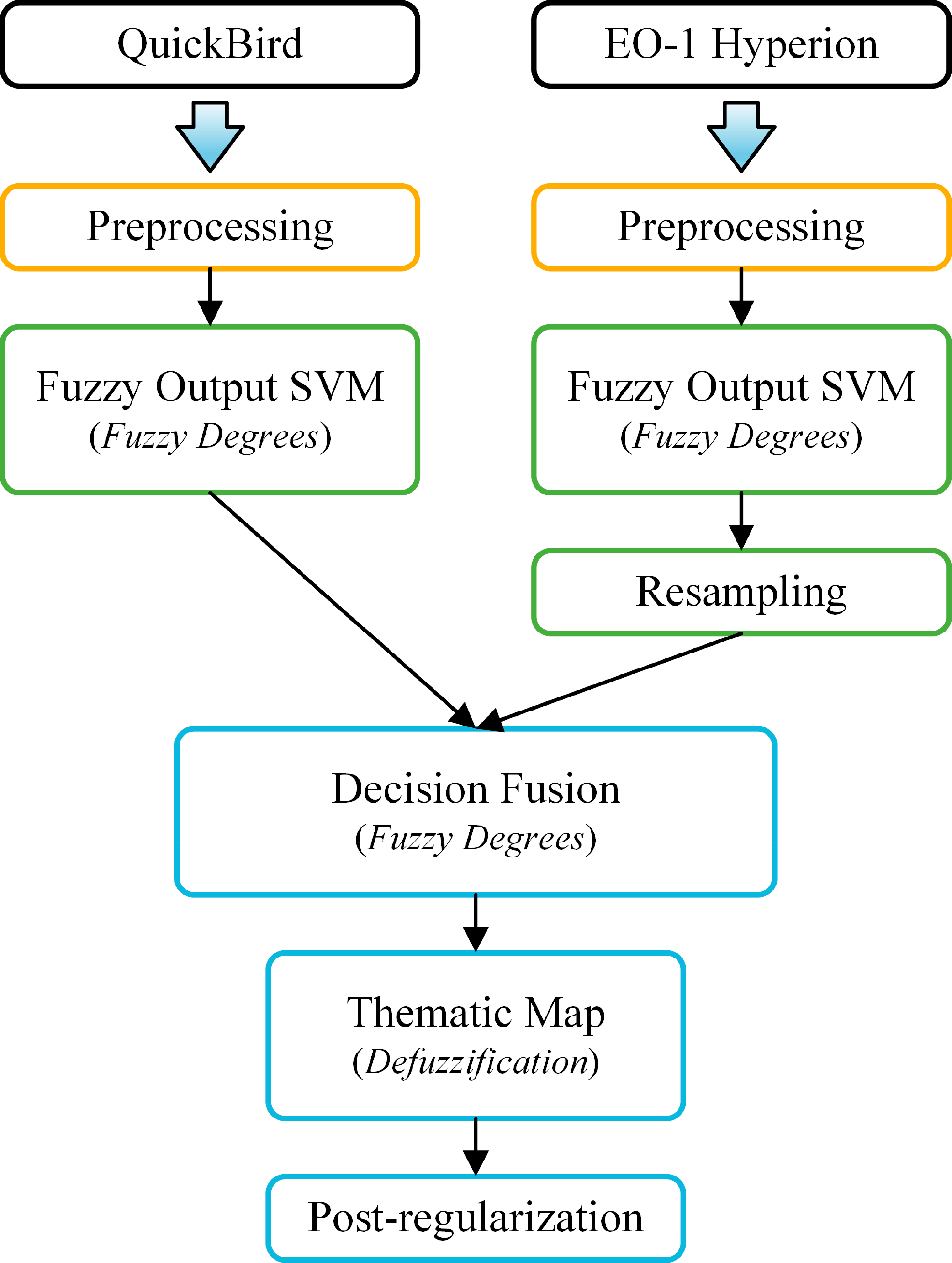
Figure 4 presents the spectral signature of each class for the Hyperion and QuickBird images. Each curve has been created by calculating each band’s median digital number (DN) over all testing pixels belonging to the respective class. The bands are represented by their nominal central wavelength. The reported central wavelength values for QuickBird are the mean values of each band’s spectral range, as determined by the sensor’s technical description sheet. Although pixels of the same class have different spectral responses in general, the median values are—to some extent—representative of each sensor’s discriminating capabilities. From Figure 4b it is evident that the two pine classes cannot be easily separated from the QuickBird dataset alone, whereas some bands of the Hyperion image provide higher discrimination, mostly in the NIR portion of the spectrum. On the other hand, the QuickBird data provide higher discrimination for the Italian Oak and Beech classes, especially in the NIR band. To this end, fusion of the two data sources can effectively exploit each sensor’s relative advantages, as it will be proven in Section 3.
2.4. Fuzzy Output SVM
The objective of a classifier is to perform the mapping from a certain N-dimensional feature space X ∈ ℜN to a predefined class space C = {c1,…,cM}, representing the M classes of the problem. In its original form, the support vector machine (SVM) is a binary classifier, based on the principles of the structural risk minimization theory [45,54,55]. Here we provide only a short presentation of the classifier. A thorough description can be found in the aforementioned references. Assume a set comprising Q training patterns E = {(xi,yi), i = 1,…,Q}, where xi ∈ X denotes the feature vector of the ith training pattern and yi = {−1,+1} its class label. The primary objective of SVM is to find an optimal separating hyperplane that maximizes the margin between the two classes. To facilitate searching in complex nonlinear problems, each vector xi in the original feature space is transformed into a higher-dimensional feature space F via a non-linear mapping Φ: X→F. A binary classification task is solved on the transformed feature space, constructing the optimal linear separating hyperplane. The transformation is performed through a kernel function K(xi, xj), which allows dot products to be computed in higher dimensional feature spaces, without directly mapping the data into these spaces.
Without delving into details, the decision value of a trained SVM model for any input feature vector x ∈ X to be classified is given by:
The one-versus-one (OVO) and the one-versus-rest (OVR) are the two strategies most frequently employed to extend SVM to multiclass problems. The first one constructs M(M − 1)/2 binary classifiers, one for each possible pairs of classes. The final decision is inferred through majority voting between the elemental binary classifiers. The OVR strategy constructs M binary SVMs, one for each class. Each elemental classifier is trained considering the patterns of the respective class as positive ones and the rest as negative. Given a feature vector x ∈ X to be classified, we obtain a vector of decision values:
The fuzzy output SVM (FO-SVM) also provides a membership degree in the range [0,1] for each class (along with the crisp classification decision), where the jth degree value denotes the certainty that an input pattern belongs to class cj. Deriving fuzzy degrees from individual decision values is possible under both multiclass strategies [56–60]. In this study, we employ the OVR multiclass strategy and derive SVM’s continuous output following the methodology proposed in [60]. Specifically, each input instance x ∈ X to be classified is assigned a fuzzy membership degree μj (x) ∈ [0,1] for each class, calculated through the relation:
Effectively, the fuzzy degree for the jth class does not depend solely on the decision value of the respective classifier, but also on the decision value of the maximum competitor. The instance x is finally assigned to the class exhibiting the highest membership grade, which is mathematically expressed as:
As shown in Figure 1, the previously described FO-SVM is applied to the Hyperion and QuickBird datasets independently. In each case, all features are normalized in the range [0,1], since SVM uses a common kernel parameter γ for all input dimensions (see Equation (2)). The optimal training parameters (C, γ) are determined through a 3-fold cross-validation procedure, using a grid of possible values for each parameter. Ultimately, the pair (Copt, γopt) that maximizes the cross-validation accuracy is selected and the classifier is trained using the whole training set.
The application of FO-SVM on the two satellite images results in two fuzzy thematic map being produced, each comprising M fuzzy images, one for each class. The kth fuzzy image can be interpreted as the certainty or possibility map of the classifier for the respective class. Note that the notion of the certainty degree does not coincide with the concept of probability. The latter has a stricter definition, requiring that the probabilities for all classes add to one. Nevertheless, obtaining probability estimates from decision values is also possible [61,62].
2.5. Decision Fusion
Decision fusion is the process of combining the outputs of multiple classifiers in order to achieve higher accuracy on a given classification task. The same basic concept has been given various names in the literature [63], amongst which the terms classifier fusion, classifier combination, multiple classifier system, and classifier ensemble are the most common. Even more are the different fusion operators that have been proposed in the literature, ranging from simple arithmetic operations to more complex combiners such as fuzzy integrals, decision templates, even genetic algorithms-based schemes, to only name a few [64–68].
In the respective literature, various fusion operators have been proposed, that can be applied both to crisp labels and the soft output of the classifiers [69]. However, crisp combiners are primarily effective when fusing multiple classifiers, whereas their accuracy decreases when combining only two classifiers. In fact, some of them cannot infer decisions when the two classifiers disagree or will always output the decision of one of the classifiers, such as the majority voting and weighted majority voting combiners, which are the most well-known operators employed for crisp labels. This is the reason which impelled us to utilize a soft output classifier (the FO-SVM described in the previous subsection) in this study and employ a soft output fusion operator. Comparing different fusion operators is outside the scope of this study. Instead, a simple and commonly applied soft combiner has been chosen to perform the fusion, namely, the weighted average rule. Actually, the weighted average combiner is the most widely used fusion operator, due to its simplicity and consistently good performance on a variety of classification tasks [64,70].
As shown in Figure 1, applying the FO-SVM classifier on the Hyperion and the QuickBird datasets results in two fuzzy thematic maps being created. The Hyperion map is subsequently resampled and registered to QuickBird’s spatial resolution, using a nearest neighbor rule. On the implementation level, all pixels of the new image (with 2.4 m spatial resolution) the center of which lie inside an original Hyperion pixel (with 30 m spatial resolution) receive the membership degrees of the original pixel. Therefore, for each pixel x (in the final resolution) we are provided with two vectors of memberships degrees for all classes μhyp(x) and μqck(x), originating from the Hyperion and the QuickBird classification, respectively. The elements of each vector is obtained through Equation (4). The weighted average combiner produces a new vector of membership values μfus(x), the jth (j = 1,…,M) of which is calculated through:
The weights signify the importance of each classifier in the final decision and are estimated through class-specific accuracy measures, typically through metrics derived from a confusion matrix, such as producer’s accuracy (PA) and user’s accuracy (UA) [71]. In this study, we follow the approach used in [20], employing the so-called F-measure that combines both metrics:
The respective weights are defined through a normalization of the F-measures, so that :
Note that the normalization does not affect the final decision. However, it assures that all final membership degrees are confined in the range [0,1].
The weighted average rule belongs to the class of the so-called trainable combiners [64], owing to the fact that the associated weights must be specified through dataset-derived metrics. These weights must be reliable estimators of the importance of each classifier in the final decision. To this end, we calculate the respective F-measures (Equation (9)) on a validation set of examples (see Table 1), different from the dataset used to train the classifiers. This approach reduces the probability of overfitting the fusion operation, since the class-specific metrics on the validation set are better representatives of each classifier’s true generalization capabilities.
As noted in Section 2.3, the Hyperion dataset includes extra training patterns for the shadows class, whereas the QuickBird training dataset only comprises the first six classes of Table 1. Before applying the fusion operator, the corresponding shadow component of Hyperion’s fuzzy thematic map is discarded, whereas the rest of the membership degrees are kept intact. These pixels practically receive the class specified by the QuickBird classification. Theoretically there exist the possibility that a pixel characterized as shadow will obtain a different label than QuickBird’s decision, which occurs if some other class exhibits sufficiently higher membership grade that the equivalent QuickBird’s one. This is, however, practically rather improbable, since shadows are easily discriminated from other classes, leading to a high membership grade only for the shadow component. Discarding the shadow component is intuitively justifiable: since the Hyperion classification cannot infer a decision about the land cover type of the respective area, the final decision is taken by the QuickBird classification, which is capable of providing that information. The respective pixels will exhibit lower membership grades in the fused fuzzy thematic map though. This behavior also seems intuitively correct, since classifications based on only one classifier are expected to exhibit lower certainty degrees.
We should finally note that the portions of the study area covered by the QuickBird but not the Hyperion imagery (see Figure 3a,b) cause no problems in the fusion process. This areas will directly receive QuickBird’s classification decision (with lower membership grades), since for those areas it holds by definition that μhyp(x) = 0.
2.6. Post-Regularization
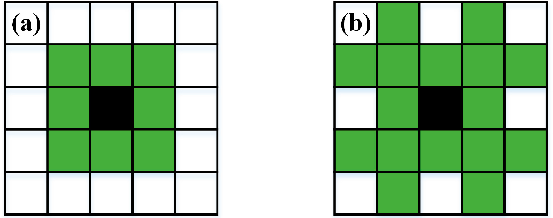
Pixel-based classifications using high spatial resolution imagery typically suffer from high levels of noise in the classification, a phenomenon commonly referred to as salt-and-pepper effect. A simple and computationally efficient way to reduce the extent of this phenomenon is to post-process the final thematic map, applying some form of spatial low-pass filtering. In this study, we employ the simple but effective post-processing scheme proposed in [72], called post-regularization (PR). As shown in Figure 1, PR is the last step of the proposed methodology. The final thematic map is filtered using the masks shown in Figure 5, which are 8- and 16-neighborhoods of a pixel, called Chamfer neighborhoods. Each pixel in the classification map is filtered using Chamfer sliding windows. PR is a three-step procedure:
- (1)
If more than T1 neighbors in the 8-neighborhood (Figure 5a) have a common class label L that is different from that of the sliding window’s central pixel, its label is changed to L. Perform this filtering iteratively on all pixels of the map until stability is reached (none of the pixels changes its label).
- (2)
If more than T2 neighbors in the 16-neighborhood (Figure 5b) have a common class label L that is different from that of the sliding window’s central pixel, its label is changed to L. Perform this filtering until stability is reached.
- (3)
Repeat the regularization process on the 8-neighborhood with threshold T3 (Step 1).
The PR step results in more homogeneous regions in the classification map. Since the objective of the present study is mapping forest species and the spatial resolution of the final thematic map is 2.4 m, the probability of removing a significant structure through PR is marginal (if existent at all). Following the recommendations of [72], the threshold values have been set to T1 = T3 = 5 and T2 = 12, which are considered as being a good tradeoff between filtering the noise and minimizing the risk of losing small but significant objects in the classification map.
Throughout the experimental results section, classification accuracies will be given in each case both before and after the PR procedure. Its effect will also be validated through visual comparisons between the respective thematic maps. We should note that the application of the PR on the resampled Hyperion classification map with the threshold values specified above does not have any effect, since an original Hyperion pixel corresponds to 12.5 pixels in the 2.4 m spatial resolution of the resampled image. If we apply the PR filtering on the original Hyperion classification map, its accuracy will decrease significantly, due to the low spatial resolution of 30 m. Therefore, the PR procedure is always applied on the finer spatial resolution thematic map.
3. Results and Discussion
3.1. Performance of the Proposed Decision Fusion Approach
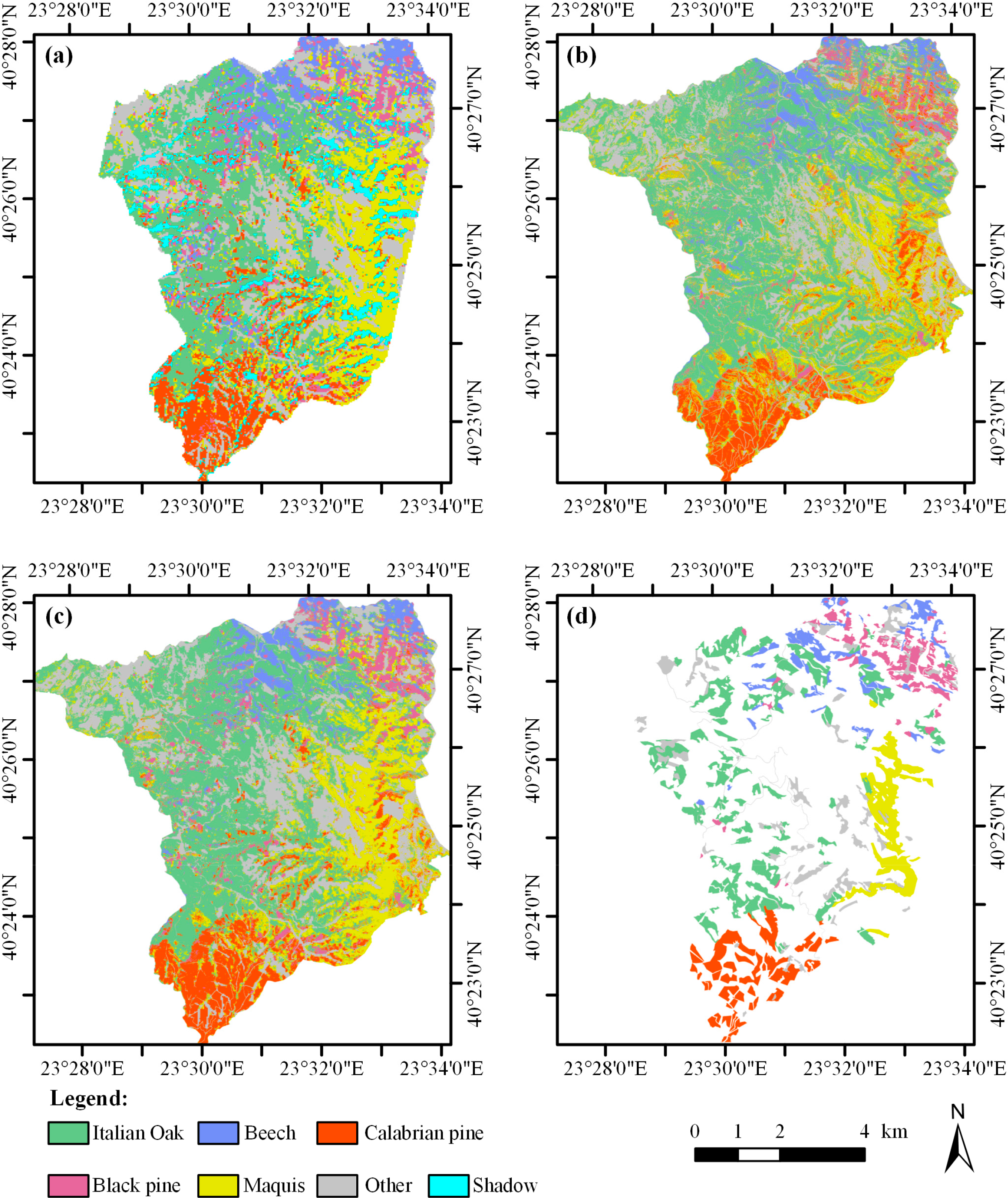
Forest species maps produced from the application of FO-SVM on the Hyperion and the QuickBird datasets, as well as the proposed decision fusion approach are depicted in Figure 6. In each case, the maps obtained after applying the PR filtering are shown. The equivalent accuracy assessment measures on the testing dataset are reported in Table 2. In this study, we employ both class-specific and global accuracy measures derived from the confusion matrix theory [71,73], as a means of evaluating the differences between the various approaches presented. Specifically, the class-specific measures include the producer’s (PA) and user’s accuracy (UA), whereas the global metrics considered include the overall (OA) and average accuracy (AA), as well as the khat (k̂) statistic. All accuracy measures are provided both before and after applying the PR procedure. We should remind that Hyperion’s classification is unaffected by the PR filtering, as explained previously.
The obtained results indicate a substantial increase in classification accuracy through the fusion operation, both before and after the PR filtering. Observing the differences between the individual PA values is indicative of the gains’ magnitude. Even before the PR filtering, all PA values except for the Beech class are higher than those obtained even by the QuickBird dataset after PR. The increased classification accuracy does not come at the cost of generalization though (expressed through the UA measure): higher UA values are obtained after the decision fusion for four out of the six classes, whereas the UA values for the other two classes are close to the respective best values observed. Regarding the OA, a difference of approximately 10% is observed before the PR filtering compared to both single-source classifications, whereas the OA after the PR filtering is 8% higher than the equivalent accuracy obtained by the QuickBird classification. The comparison with respect to the other two global accuracy measures leads to similar conclusions. We should note that the effect of the PR filtering is much smaller in the case of the fused classification, compared to the equivalent gain observed for the QuickBird dataset, a behavior that is discussed in Section 3.2. The Hyperion classification seems to outperform the QuickBird one only for the Oak and Other classes. Yet the fused classification outperforms both single-source classifications in all six classes. This seemingly paradoxical behavior will be clarified later in Section 3.3.
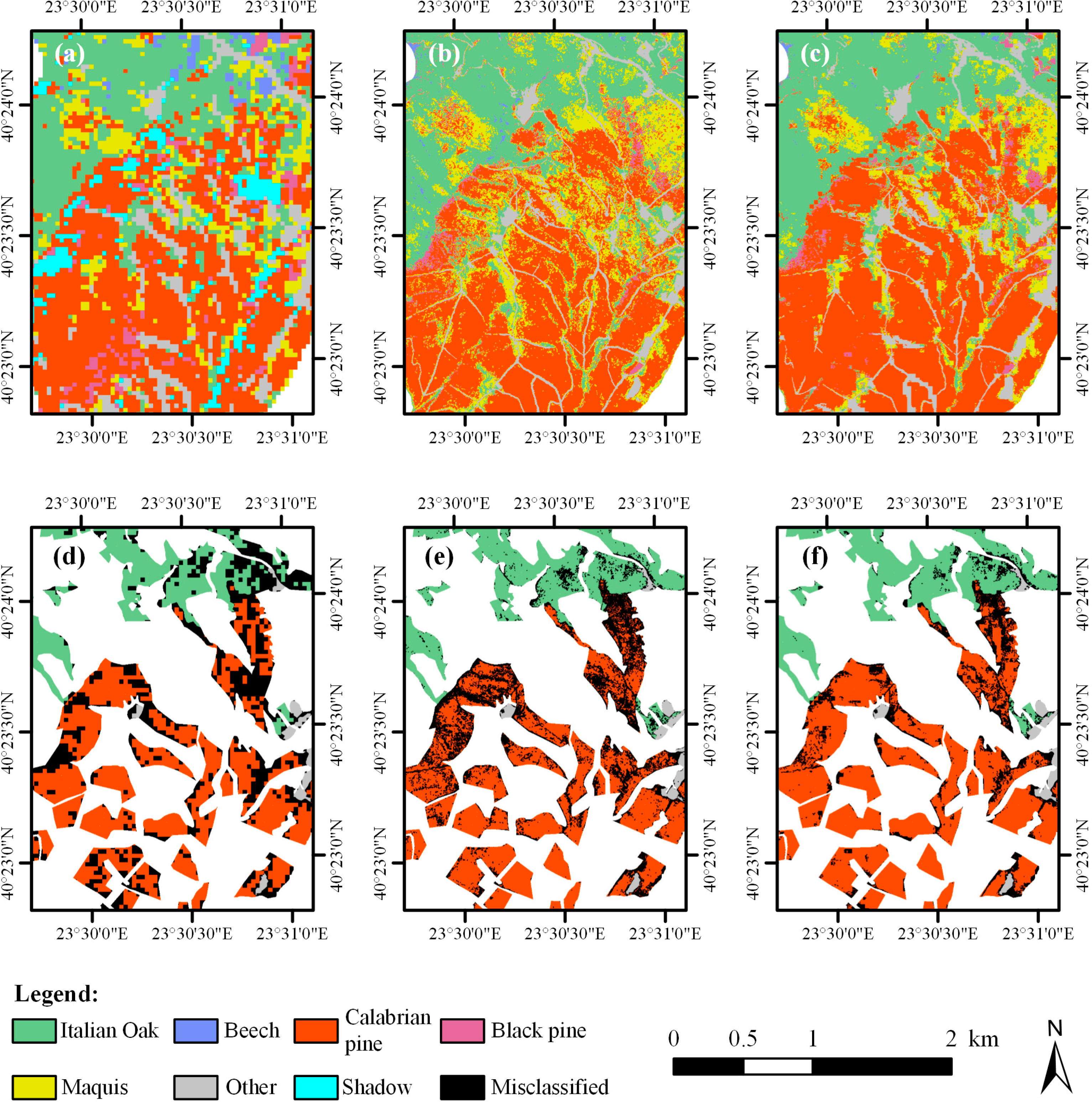
Figure 7 provides a detail of the three classification maps in a southern region of the study area, primarily covered with Calabrian pines and oaks. The second row of images depict the equivalent “error maps”. An error map is produced by showing the classification only inside the testing reference areas and highlighting misclassified pixels with black color. The advantages of combining two single-source classifiers through decision fusion is evident. The QuickBird map (Figure 7b) provides a detailed characterization of the area. However, its high spatial resolution results in heavy salt-and-pepper effects. On the other hand, the Hyperion classification (Figure 7a) provides more homogeneous characterizations, but the cost of a single misclassification is high (a single 30 m misclassified Hyperion pixel results in an area of 900 m2 being immediately characterized erroneously). Ultimately, the fused map (Figure 7c) provides homogeneous classification, preserving nevertheless QuickBird’s spatially detailed characterization. The differences are more easily observable through the equivalent error maps (Figure 7d–f). Unavoidably, areas characterized as shadows in the Hyperion classification directly receive the decision provided by the QuickBird one.
The most complex mosaic on the study area is observed in its northeastern corner, where Black pines, oaks, and beeches are intertwined with bare rocks along the steep slopes of Mount Cholomontas. A detail of the three classifications in this region is depicted in Figure 8, following the same presentation with Figure 7. The QuickBird classification is characterized by many erroneous assignments, particularly for areas covered with Black pines, which are misclassified as Calabrian pines. The proposed fusion methodology utilizes Hyperion’s higher discriminating capabilities in this region, correcting most of the misclassifications. This result confirms the findings of other studies of the literature, which—as mentioned in the introduction—testify that hyperspectral data are valuable for accurately discriminating different species of the same genus.
3.2. Contribution of the Post-Regularization Filtering
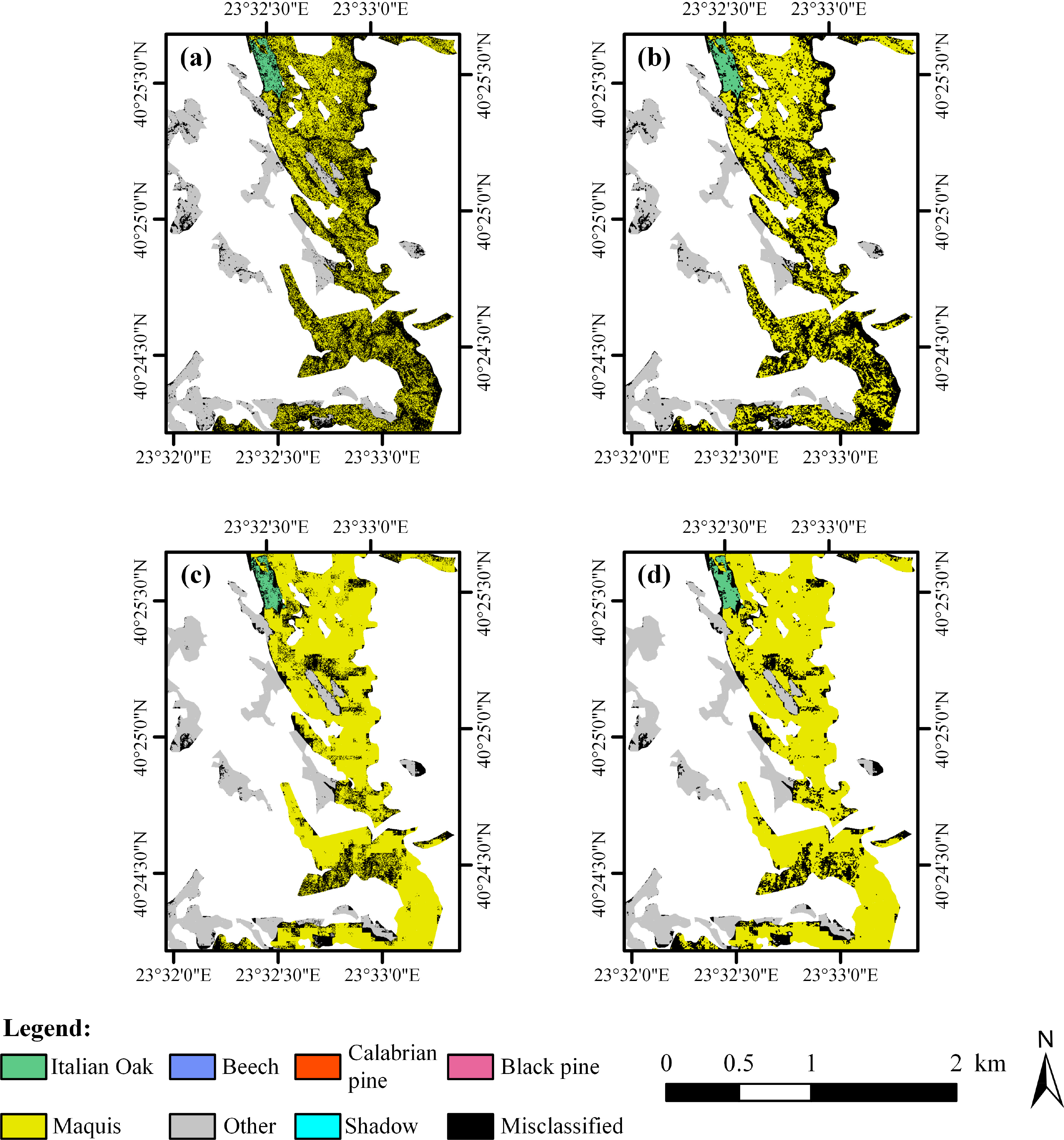
Table 2 reveals that the contribution of the PR filtering to the final classification accuracy is higher in the case of the QuickBird classification than the equivalent for the fused classification. It is therefore interesting to visually observe the differences in the classification maps prior and after applying the PR procedure. The comparison can be performed to any of the regions depicted in Figures 7 and 8. However, here we selected another region in the eastern part of the study area, where the salt-and-pepper phenomenon is even more intense than the previous cases. This area is predominantly covered with Maquis, which form sparsely distributed shrub-like low vegetation patches. The pixel-based classification of spatially sparse vegetation through VHR imagery becomes problematic, since no information on the spatial distribution and density of the underlying land cover type can be provided when considering only the initial bands of the image.
Figure 9a depicts the error map for the QuickBird classification before PR. This classification is characterized by extreme levels of noise and a high percentage of the pixels have been misclassified. Applying the PR filtering (Figure 9b) alleviates the problem to a considerable degree, but many misclassification remain, since the PR process does not evaluate any spectral information. On the other hand, the fused classification utilizes Hyperion’s coarser spatial resolution to guard from excessive noise even before the PR filtering (Figure 9c). To this end, the latter process has a noticeable but less significant contribution to the final classification map (Figure 9d). This behavior is actually desirable, since the PR algorithm is a simple iterative low-pass filtering algorithm and its post-processing capabilities are limited by the lack of any extra spectral information.
The previously described difference in the two classifications can be identified in many areas of the image (to a lesser or equal degree) and it is one of the reasons for the much lower accuracy achieved by the QuickBird classification.
3.3. Why and How Does Fusion Work?
The numeric results presented in Table 2 probably conceal the reasons of the fusion operation’s success. At first glance it may seem strange that the combination of two classifications can provide higher PA values for all associated classes than any of the elemental components. Although this behavior is frequently observed in decision fusion applications, it can easily be explained in the context of the specific application presented here. In doing so, one should keep in mind that the fuser is trained on the validation set, that is, the weights determination through Equation (10) employs the PA and UA values calculated on the validation set.
Table 3 presents the results of employing the accuracy assessment on the validation set of examples. A striking first difference relates to the relatively high discrepancies observed between all equivalent accuracy measures in the validation and testing datasets (compare with Table 2). On a first level, the difference is attributed to the fact that the testing dataset comprises a much higher number of reference patterns (approximately 2.6 million), as contrasted to validation’s 172 reference points. There exist however a further distinction arising from the different spatial resolution of the images. The QuickBird and fused classifications are affected by salt-and-pepper effect, owning to their very high resolution. The validation patterns were obtained through field inspection and are generally located in unambiguous sporadic points of the study area. On the other hand, the lower testing accuracy of Hyperion’s classification is primarily attributed to its coarse spatial resolution. As noted earlier, a misclassification of an original Hyperion pixel results in 12.52 ≈ 156 pixels on the resampled image being misclassified. Moreover, shadows are considered as misclassified pixels, further reducing the accuracy. Under this perspective, the testing accuracy values underestimate the true discriminating capabilities of the Hyperion data source. This does not mean that the testing accuracy values are misleading: the quality of the final map is indeed inhibited by the coarse spatial resolution. However, if we were able to increase Hyperion’s spatial resolution, its discriminating capabilities could be spotlighted. The decision fusion approach performs this operation, by effectively exploiting Hyperion classifications that exhibit high certainty membership grades, on a subpixel level.
The above comment can be easily depicted through visual inspection of each class membership grades. The result of applying Equation (7) on all image pixels is actually a set of M fuzzy thematic maps or certainty maps, where M is the number of classes. Each fuzzy thematic map can be directly represented as a gray-level image. However, more interesting conclusions can be drawn by intelligently exploiting the channels of an RGB image representation. The top row of Figure 10 depicts such a representation on a smaller region around the middle of the area shown in Figure 7, where the Calabrian pine and Maquis fuzzy thematic maps have been assigned to the red and green channels, respectively, of an RGB representation. Under this configuration, bright green pixels on the fuzzy maps correspond to pixels for which the classifier is very confident that they represent the Maquis class. Accordingly, bright red pixels correspond to high certainty degrees for the Calabrian pine class and at the same time low degrees for the Maquis class. Hence, an associated color map is defined, shown in Figure 10g. Mixed pixels (that is, pixels with equivalent certainty degrees for both classes) are represented by some shade of yellow, around the π/4 line in the color map.
The QuickBird fuzzy map (Figure 10a) produces high certainty degrees for only one class in each pixel, although the Maquis high certainty pixels are actually misclassifications (Figure 10d). On the other hand, some pixels on the Hyperion fuzzy map (Figure 10b) have yellowish or brownish color, which correspond to areas with mixed signatures, as a natural consequence of the coarse spatial resolution. Accordingly, a higher number of pixels in the decision fusion fuzzy map (Figure 10c) are characterized by intermediate colors, thus effectively exploiting the information provided by both sources. Consequently, the final map is characterized by homogeneous classifications, maintaining however the high spatial resolution where needed, as it is probably more easily visible in the respective classification maps (Figure 10d–e).
3.4. Comparison with Alternative Approaches
The results presented so far undeniably indicate that the fusion operation exploits Hyperion’s coarser spatial resolution to obtain a classification map with more homogeneous characterizations. A question arises naturally from the analysis: is the observed increase in accuracy also related to Hyperion’s higher spectral resolution? A second more general question might be posed: can a higher accuracy be obtained by some other form of simultaneous evaluation of the two data sources? This last subsection answers these two questions, by comparing the proposed methodology with other popular approaches.
A partial answer to the first question has been given in Section 3.3, which explained how the fusion operation effectively exploits the information provided by both sensors. Nevertheless, researcher typically avoid considering only the initial bands of VHR multispectral imagery, as the classification result is usually characterized by high salt-and-pepper effects (as shown in this study as well). A common alternative is to derive higher-order spectral and textural features from the initial image, thus infusing multi-scale spatial resolution properties in the feature space. Such an approach on VHR imagery involves high computational demands and high amounts of storage and memory requirements. Moreover, it is generally unknown in advance which feature transformations and window sizes are the optimal ones. The maximalist approach is to consider a large set of possible feature transformations and subsequently select the most important ones by means of some feature selection method [60]. To this end, we have created an enriched feature space from the initial QuickBird image, considering a number of higher-order spectral and textural transformations:
Spectral transformations (principal components analysis, the tasseled cap and intensity-hue-saturation transformations, as well as five common vegetation indices).
Four first-order textural statistics (data range, mean, variance, entropy) for each band.
Eight second-order textural statistics (mean, variance, homogeneity, contrast, dissimilarity, entropy, second moment, correlation) for each band, using the gray-level co-occurrence matrix (GLCM) transformation.
Three local indicators of spatial association (LISA) measures for each band (Geary’s, Getis-Ord, and Moran).
First order statistics and GLCMs were calculated considering four different window sizes, whereas LISA features have been calculated considering six different lags. Ultimately, 282 higher-order features have been produced, out of which the 11 most important ones were finally maintained applying a state-of-the-art powerful feature selection method, namely, Wr-SVM-FuzCoC [74]. For practical reasons, the latter dataset will be referred as Qck.HO-FS in the following.
Table 4 hosts the accuracy assessment results on the testing set for the Qck.HO-FS dataset. Compared to the initial QuickBird classification (Table 2), a very significant increase in the accuracy is observed before the PR step, which implies that the additional spatial information provided can effectively diminish the salt-and-pepper effect of the initial classification. However, the PR filtering cannot increase the final accuracy any further, since all noise has been removed from the classification map through the sliding window-based spatial information. Therefore, the final accuracy is less than 2% higher than QuickBird’s initial classification. Table 2 also reports the results of applying the proposed methodology on the new dataset, that is, fusing the Hyperion and the Qck.HO-FS classification maps. A significant increase of more than 6% is observed after PR, which is nevertheless equivalent to the performance of the initial fusion operation. The last example proves that the proposed methodology exploits both the coarser spatial resolution and the finer spectral resolution of Hyperion’s data. In addition, an equivalent result can be obtained by fusing the initial (bands only) classifications, without having to resort to the extremely time-consuming and computationally demanding operation of higher-order spatial feature extraction.
To answer the second question (whether a higher accuracy can be obtained by some other form of data fusion), we devised additional experiments considering the popular vector stacking approach, which concatenates the inputs of the two sources directly, forming a composite feature space. We identify three possible scenarios:
VS1: Concatenating the 155 bands of the Hyperion image with the four initial bands of the QuickBird one.
VS2: Concatenating the 155 bands of the Hyperion image with the Qck.HO-FS dataset described previously.
VS3: Concatenating the 155 bands of the Hyperion image with all 282 features derived from the QuickBird image, forming an initial space with 437 features. Subsequently, we employ the previously mentioned feature selection method (Wr-SVM-FuzCoC), resulting in the 30 most important features being selected.
We should note that all the above vector stacking approaches require the initial Hyperion image to be resampled to QuickBird’s spatial resolution, which in turn require very high amounts of computer storage and memory.
Table 5 hosts the results obtained by the three vector stacking approaches on the testing dataset. The table reports the accuracy values only after the PR filtering, since the equivalent values before PR were marginally lower. In all cases, an increase of the classification accuracy is observed compared to the initial Hyperion and QuickBird classifications (see Table 2). Nevertheless, the final accuracy obtained by any vector stacking approach is significantly lower than the proposed decision fusion approach, a fact that proves that fusion on the decision level has a higher degree of flexibility.
Figure 11 presents a detail of the classification maps obtained by the various approaches. Regarding the three vector stacking approaches, VS3 (Figure 11c) exhibits a rather higher quality map than VS1 (Figure 11a) and VS2 (Figure 11b), which seem to be highly affected by Hyperion’s coarse spatial resolution. Nevertheless, VS3 resulted in many misclassification of Calabrian pine pixels, which were assigned to Maquis and Black pine. The Qck.HO-FS classification shows even higher levels overestimation of the Maquis class (Figure 11d), although the salt-and-pepper effect of the initial QuickBird classification has been diminished. On the other hand, the proposed methodology (Figure 11e) results in accurate forest species mapping, maintaining QuickBird’s detailed classification but removing most of the associated thematic map noise at the same time.
4. Notes on Operational Usability
The previous section showcased the proposed methodology’s effectiveness in delivering increased classification accuracy in complex forest landscapes. Here we provide some additional comments regarding its usability from an operational perspective.
The fusion operator adopted in this study was deliberately chosen to be a simple one, so that the proposed methodology can be easily applied in practice. Indeed, the weighted average scheme can be implemented through simple band math operations, readily provided by many—commercial and not—GIS software applications. The only requirement imposed is for the classification algorithm to support some form of soft output. A fuzzy output is not a prerequisite of the methodology; any soft output classifier can be used. For example, imageSVM [75] is a freely available IDL/ENVI application that serves as a convenient frontend to the LIBSVM library [76] (the most popular freely distributed implementation of SVM, also used by the current study). Although we did not test it ourselves, imageSVM’s manual reports that the application can also output the posterior probabilities for each pixel classification, which can be directly used to apply the methodology presented in this study.
An important finding of the present study is that satellite hyperspectral imagery can be extremely useful in complex terrains mapping, if combined with a VHR imagery. This is a cost-effective solution for increasing the mapping accuracy, since the airborne hyperspectral sensors commonly employed in recent remote sensing applications involve much higher costs than satellite imagery. It is true that the currently only available spaceborne sensor (Hyperion) offers moderate spectral stability measurements [52], with some bands exhibiting high degree of noise and/or random stripes. Nevertheless, a number of spaceborne hyperspectral sensors will be available in the very near future [42–44], rendering the proposed methodology extremely useful for accurate and fast characterizations of large areas.
5. Conclusions
This study presented a simple yet effective methodology for accurate forest species mapping, combining the complementary information provided from a multispectral and a hyperspectral satellite image. The basic idea is to initially obtain two independent fuzzy classifications from each source, employing a fuzzy output version of the SVM classifier. The two fuzzy classifications are then combined through a proper decision fusion operator and the final thematic map is obtained after the application of a simple post-processing filtering procedure, which eliminates the remaining noise. The methodology was tested on a challenging forest species mapping task, characterized by high degree of inter-species spatial mixing. The thorough experimental analysis has proven the effectiveness of the proposed methodology in obtaining accurate classification maps, through the simultaneous exploitation of the multispectral image’s high spatial resolution and the hyperspectral image’s detailed spectral information. Even more importantly, common alternative approaches for exploiting both data sources have proven significantly inferior in terms of classification accuracy and quality of the derived thematic maps, even though their computational demands are much higher.
Acknowledgments
This research has received funding by the European Union (European Social Fund-ESF) and Greek national funds through the Operational Program “Education and Lifelong Learning” of the National Strategic Reference Framework (NSRF) Research Funding Program: THALES. Investing in knowledge society through the European Social Fund.
The EO-1 Hyperion data used were available at no cost from the US Geological Survey.
Author Contributions
Dimitris Stavrakoudis proposed the employed methodology and developed the research design, performed the experimental analysis, manuscript writing, and results interpretation. Eleni Dragozi performed the image preprocessing, contributed to the delineation of the testing reference areas, and contributed to manuscript revision. Ioannis Gitas contributed to research design, optical image processing, results interpretation, discussion writing and manuscript revision. Christos Karydas contributed to the interpretation of the very high spatial resolution image (before and after classification), the reference data evaluation, and interpretation of ambiguous classifications, and manuscript writing.
Conflicts of Interest
The authors declare no conflict of interest.
References
- Kosaka, N.; Akiyama, T.; Tsai, B.; Kojima, T. Forest type classification using data fusion of multispectral and panchromatic high-resolution satellite imageries. Proceedings of the 2005 IEEE International Geoscience and Remote Sensing Symposium, IGARSS ’05, Seoul, Korea, 25–29 July 2005; 4, pp. 2980–2983.
- Wang, L.; Sousa, W.P.; Gong, P.; Biging, G.S. Comparison of IKONOS and QuickBird images for mapping mangrove species on the Caribbean coast of Panama. Remote Sens. Environ 2004, 91, 432–440. [Google Scholar]
- Goodenough, D.G.; Dyk, A.; Niemann, K.O.; Pearlman, J.S.; Chen, H.; Han, T.; Murdoch, M.; West, C. Processing Hyperion and ALI for forest classification. IEEE Trans. Geosci. Remote Sens 2003, 41, 1321–1331. [Google Scholar]
- Govender, M.; Chetty, K.; Naiken, V.; Bulcock, H. A comparison of satellite hyperspectral and multispectral remote sensing imagery for improved classification and mapping of vegetation. Water SA 2008, 34, 147–154. [Google Scholar]
- Stavrakoudis, D.G.; Galidaki, G.N.; Gitas, I.Z.; Theocharis, J.B. A genetic fuzzy-rule-based classifier for land cover classification from hyperspectral imagery. IEEE Trans. Geosci. Remote Sens 2012, 50, 130–148. [Google Scholar]
- Dalponte, M.; Bruzzone, L.; Gianelle, D. Fusion of hyperspectral and LIDAR remote sensing data for classification of complex forest areas. IEEE Trans. Geosci. Remote Sens 2008, 46, 1416–1427. [Google Scholar]
- Clark, M.L.; Roberts, D.A.; Clark, D.B. Hyperspectral discrimination of tropical rain forest tree species at leaf to crown scales. Remote Sens. Environ 2005, 96, 375–398. [Google Scholar]
- Leckie, D.G.; Tinis, S.; Nelson, T.; Burnett, C.; Gougeon, F.A.; Cloney, E.; Paradine, D. Issues in species classification of trees in old growth conifer stands. Can. J. Remote Sens 2005, 31, 175–190. [Google Scholar]
- Yokoya, N.; Mayumi, N.; Iwasaki, A. Cross-calibration for data fusion of EO-1/Hyperion and Terra/ASTER. IEEE J. Sel. Top. Appl. Earth Obs. Remote Sens 2013, 6, 419–426. [Google Scholar]
- Chen, Z.; Pu, H.; Wang, B.; Jiang, G.-M. Fusion of hyperspectral and multispectral images: A novel framework based on generalization of pan-sharpening methods. IEEE Geosci. Remote Sens. Lett 2014, 11, 1418–1422. [Google Scholar]
- Song, H.; Huang, B.; Zhang, K.; Zhang, H. Spatio-spectral fusion of satellite images based on dictionary-pair learning. Inf. Fusion 2014, 18, 148–160. [Google Scholar]
- Bruzzone, L.; Prieto, D.F.; Serpico, S.B. A neural-statistical approach to multitemporal and multisource remote-sensing image classification. IEEE Trans. Geosci. Remote Sens 1999, 37, 1350–1359. [Google Scholar]
- Amarsaikhan, D.; Douglas, T. Data fusion and multisource image classification. Int. J. Remote Sens 2004, 25, 3529–3539. [Google Scholar]
- Huang, X.; Zhang, L.; Gong, W. Information fusion of aerial images and LIDAR data in urban areas: Vector-stacking, re-classification and post-processing approaches. Int. J. Remote Sens 2011, 32, 69–84. [Google Scholar]
- Dalponte, M.; Bruzzone, L.; Gianelle, D. Tree species classification in the Southern Alps based on the fusion of very high geometrical resolution multispectral/hyperspectral images and LiDAR data. Remote Sens. Environ 2012, 123, 258–270. [Google Scholar]
- Ghosh, A.; Fassnacht, F.E.; Joshi, P.K.; Koch, B. A framework for mapping tree species combining hyperspectral and LiDAR data: Role of selected classifiers and sensor across three spatial scales. Int. J. Appl. Earth Obs. Geoinf 2014, 26, 49–63. [Google Scholar]
- Pedergnana, M.; Marpu, P.R.; Dalla Mura, M.; Benediktsson, J.A.; Bruzzone, L. Classification of remote sensing optical and LiDAR data using extended attribute profiles. IEEE J. Sel. Top. Signal Process 2012, 6, 856–865. [Google Scholar]
- Fauvel, M.; Chanussot, J.; Benediktsson, J.A.; Sveinsson, J.R. Spectral and spatial classification of hyperspectral data using SVMs and morphological profiles. Proceedings of the 2007 IEEE International Geoscience and Remote Sensing Symposium, IGARSS 2007, Barcelona, Spain, 23–27 July 2007; pp. 4834–4837.
- Fauvel, M.; Benediktsson, J.A.; Chanussot, J.; Sveinsson, J.R. Spectral and spatial classification of hyperspectral data using SVMs and morphological profiles. IEEE Trans. Geosci. Remote Sens 2008, 46, 3804–3814. [Google Scholar]
- Huang, X.; Zhang, L. A multilevel decision fusion approach for urban mapping using very high-resolution multi/hyperspectral imagery. Int. J. Remote Sens 2012, 33, 3354–3372. [Google Scholar]
- Huang, X.; Zhang, L. Comparison of vector stacking, multi-SVMs fuzzy output, and multi-SVMs voting methods for multiscale VHR urban mapping. IEEE Geosci. Remote Sens. Lett 2010, 7, 261–265. [Google Scholar]
- Mitrakis, N.E.; Topaloglou, C.A.; Alexandridis, T.K.; Theocharis, J.B.; Zalidis, G.C. Decision fusion of GA self-organizing neuro-fuzzy multilayered classifiers for land cover classification using textural and spectral features. IEEE Trans. Geosci. Remote Sens 2008, 46, 2137–2152. [Google Scholar]
- Huang, X.; Zhang, L.; Wang, L. Evaluation of morphological texture features for mangrove forest mapping and species discrimination using multispectral IKONOS imagery. IEEE Geosci. Remote Sens. Lett 2009, 6, 393–397. [Google Scholar]
- Dalla Mura, M.; Villa, A.; Benediktsson, J.A.; Chanussot, J.; Bruzzone, L. Classification of hyperspectral images by using extended morphological attribute profiles and independent component analysis. IEEE Geosci. Remote Sens. Lett 2011, 8, 542–546. [Google Scholar]
- Jimenez, L.O.; Morales-Morell, A.; Creus, A. Classification of hyperdimensional data based on feature and decision fusion approaches using projection pursuit, majority voting, and neural networks. IEEE Trans. Geosci. Remote Sens 1999, 37, 1360–1366. [Google Scholar]
- Benediktsson, J.A.; Ceamanos Garcia, X.; Waske, B.; Chanussot, J.; Sveinsson, J.R.; Fauvel, M. Ensemble methods for classification of hyperspectral data. Proceedings of the 2008 IEEE International Geoscience and Remote Sensing Symposium, IGARSS 2008, Boston, MA, USA, 7–11 July 2008; 1, pp. I:62–I:65.
- Prasad, S.; Bruce, L.M. Decision fusion with confidence-based weight assignment for hyperspectral target recognition. IEEE Trans. Geosci. Remote Sens 2008, 46, 1448–1456. [Google Scholar]
- Ceamanos, X.; Waske, B.; Benediktsson, J.A.; Chanussot, J.; Fauvel, M.; Sveinsson, J.R. A classifier ensemble based on fusion of support vector machines for classifying hyperspectral data. Int. J. Image Data Fusion 2010, 1, 293–307. [Google Scholar]
- Maghsoudi, Y.; Valadan Zoej, M.J.; Collins, M. Using class-based feature selection for the classification of hyperspectral data. Int. J. Remote Sens 2011, 32, 4311–4326. [Google Scholar]
- Fauvel, M.; Chanussot, J.; Benediktsson, J.A. Decision fusion for the classification of urban remote sensing images. IEEE Trans. Geosci. Remote Sens 2006, 44, 2828–2838. [Google Scholar]
- Doan, H.T.X.; Foody, G.M. Increasing soft classification accuracy through the use of an ensemble of classifiers. Int. J. Remote Sens 2007, 28, 4609–4623. [Google Scholar]
- Foody, G.M.; Boyd, D.S.; Sanchez-Hernandez, C. Mapping a specific class with an ensemble of classifiers. Int. J. Remote Sens 2007, 28, 1733–1746. [Google Scholar]
- Benediktsson, J.A.; Swain, P.H. Consensus theoretic classification methods. IEEE Trans. Syst. Man Cybern 1992, 22, 688–704. [Google Scholar]
- Benediktsson, J.A.; Sveinsson, J.R.; Swain, P.H. Hybrid consensus theoretic classification. IEEE Trans. Geosci. Remote Sens 1997, 35, 833–843. [Google Scholar]
- Briem, G.J.; Benediktsson, J.A.; Sveinsson, J.R. Multiple classifiers applied to multisource remote sensing data. IEEE Trans. Geosci. Remote Sens 2002, 40, 2291–2299. [Google Scholar]
- Benediktsson, J.A.; Kanellopoulos, I. Classification of multisource and hyperspectral data based on decision fusion. IEEE Trans. Geosci. Remote Sens 1999, 37, 1367–1377. [Google Scholar]
- Waske, B.; Benediktsson, J.A. Fusion of support vector machines for classification of multisensor data. IEEE Trans. Geosci. Remote Sens 2007, 45, 3858–3866. [Google Scholar]
- Waske, B.; van der Linden, S. Classifying multilevel imagery from sar and optical sensors by decision fusion. IEEE Trans. Geosci. Remote Sens 2008, 46, 1457–1466. [Google Scholar]
- Bruzzone, L.; Cossu, R.; Vernazza, G. Combining parametric and non-parametric algorithms for a partially unsupervised classification of multitemporal remote-sensing images. Inf. Fusion 2002, 3, 289–297. [Google Scholar]
- Bruzzone, L.; Cossu, R.; Vernazza, G. Detection of land-cover transitions by combining multidate classifiers. Pattern Recognit. Lett 2004, 25, 1491–1500. [Google Scholar]
- Ungar, S.G.; Pearlman, J.S.; Mendenhall, J.A.; Reuter, D. Overview of the Earth Observing One (EO-1) mission. IEEE Trans. Geosci. Remote Sens 2003, 41, 1149–1159. [Google Scholar]
- Stuffler, T.; Kaufmann, C.; Hofer, S.; Förster, K.P.; Schreier, G.; Mueller, A.; Eckardt, A.; Bach, H.; Penné, B.; Benz, U.; et al. The EnMAP hyperspectral imager—An advanced optical payload for future applications in Earth observation programs. Acta Astronaut 2007, 61, 115–120. [Google Scholar]
- Stefano, P.; Angelo, P.; Simone, P.; Filomena, R.; Federico, S.; Tiziana, S.; Umberto, A.; Vincenzo, C.; Acito, N.; Marco, D.; et al. The PRISMA hyperspectral mission: Science activities and opportunities for agriculture and land monitoring. In Proceedings of the 2013 IEEE International Geoscience and Remote Sensing Symposium (IGARSS), Melbourne, Australia, 21–26 July 2013; pp. 4558–4561.
- Devred, E.; Turpie, K.R.; Moses, W.; Klemas, V.V.; Moisan, T.; Babin, M.; Toro-Farmer, G.; Forget, M.-H.; Jo, Y.-H. Future retrievals of water column bio-optical properties using the Hyperspectral Infrared Imager (HyspIRI). Remote Sens 2013, 5, 6812–6837. [Google Scholar]
- Vapnik, V.N. Statistical Learning Theory; Wiley: New York, NY, USA, 1998. [Google Scholar]
- Mountrakis, G.; Im, J.; Ogole, C. Support vector machines in remote sensing: A review. ISPRS J. Photogramm. Remote Sens 2011, 66, 247–259. [Google Scholar]
- Melgani, F.; Bruzzone, L. Classification of hyperspectral remote sensing images with support vector machines. IEEE Trans. Geosci. Remote Sens 2004, 42, 1778–1790. [Google Scholar]
- Camps-Valls, G.; Bruzzone, L. Kernel-based methods for hyperspectral image classification. IEEE Trans. Geosci. Remote Sens 2005, 43, 1351–1362. [Google Scholar]
- Dalponte, M.; Bruzzone, L.; Vescovo, L.; Gianelle, D. The role of spectral resolution and classifier complexity in the analysis of hyperspectral images of forest areas. Remote Sens. Environ 2009, 113, 2345–2355. [Google Scholar]
- Mallinis, G.; Galidaki, G.; Gitas, I. A comparative analysis of EO-1 Hyperion, Quickbird and Landsat TM imagery for fuel type mapping of a typical Mediterranean landscape. Remote Sens 2014, 6, 1684–1704. [Google Scholar]
- Mallinis, G.; Koutsias, N.; Tsakiri-Strati, M.; Karteris, M. Object-based classification using Quickbird imagery for delineating forest vegetation polygons in a Mediterranean test site. ISPRS J. Photogramm. Remote Sens 2008, 63, 237–250. [Google Scholar]
- Middleton, E.M.; Ungar, S.G.; Mandl, D.J.; Ong, L.; Frye, S.W.; Campbell, P.E.; Landis, D.R.; Young, J.P.; Pollack, N.H. The earth observing one (EO-1) satellite mission: Over a decade in space. IEEE J. Sel. Top. Appl. Earth Obs. Remote Sens 2013, 6, 243–256. [Google Scholar]
- Datt, B.; McVicar, T.R.; van Niel, T.G.; Jupp, D.L.B.; Pearlman, J.S. Preprocessing EO-1 Hyperion hyperspectral data to support the application of agricultural indexes. IEEE Trans. Geosci. Remote Sens 2003, 41, 1246–1259. [Google Scholar]
- Cortes, C.; Vapnik, V. Support-vector networks. Mach. Learn 1995, 20, 273–297. [Google Scholar]
- Burges, C.J.C. A tutorial on support vector machines for pattern recognition. Data Min. Knowl. Discov 1998, 2, 121–167. [Google Scholar]
- Inoue, T.; Abe, S. Fuzzy support vector machines for pattern classification. In Proceedings of the International Joint Conference on Neural Networks, 2001, IJCNN ’01, Washington, DC, USA, 15–19 July 2001; 2, pp. 1449–1454.
- Borasca, B.; Bruzzone, L.; Carlin, L.; Zusi, M. A fuzzy-input fuzzy-output SVM technique for classification of hyperspectral remote sensing images. In Proceedings of the 7th Nordic Signal Processing Symposium, 2006, NORSIG 2006, Reykjavik, Iceland, 7–9 June 2006; pp. 2–5.
- Xie, Z.; Hu, Q.; Yu, D. Fuzzy output support vector machines for classification. In Advances in Natural Computation; Wang, L., Chen, K., Ong, Y.S., Eds.; Springer: Berlin/Heidelberg, Germany, 2005; pp. 1190–1197. [Google Scholar]
- Thiel, C.; Scherer, S.; Schwenker, F. Fuzzy-input fuzzy-output one-against-all support vector machines. In Knowledge-Based Intelligent Information and Engineering Systems; Apolloni, B., Howlett, R.J., Jain, L., Eds.; Springer: Berlin/Heidelberg, Germany, 2007; pp. 156–165. [Google Scholar]
- Moustakidis, S.; Mallinis, G.; Koutsias, N.; Theocharis, J. B.; Petridis, V. SVM-based fuzzy decision trees for classification of high spatial resolution remote sensing images. IEEE Trans. Geosci. Remote Sens 2012, 50, 149–169. [Google Scholar]
- Platt, J.C. Probabilistic outputs for support vector machines and comparisons to regularized likelihood methods. In Advances in Large Margin Classifiers; Smola, A., Bartlett, P., Schölkopf, B., Schuurmans, D., Eds.; MIT Press: Cambridge, MA, USA, 1999; pp. 61–74. [Google Scholar]
- Lin, H.-T.; Lin, C.-J.; Weng, R.C. A note on Platt’s probabilistic outputs for support vector machines. Mach. Learn 2007, 68, 267–276. [Google Scholar]
- Kuncheva, L.I.; Bezdek, J.C.; Duin, R.P.W. Decision templates for multiple classifier fusion: An experimental comparison. Pattern Recognit 2001, 34, 299–314. [Google Scholar]
- Kuncheva, L.I. Combining Pattern Classifiers: Methods and Algorithms; John Wiley & Sons: Hoboken, NJ, USA, 2004. [Google Scholar]
- Kuncheva, L.I. Using measures of similarity and inclusion for multiple classifier fusion by decision templates. Fuzzy Sets Syst 2001, 122, 401–407. [Google Scholar]
- Ruta, D.; Gabrys, B. An overview of classifier fusion methods. Comput. Inf. Syst 2000, 7, 1–10. [Google Scholar]
- Gabrys, B.; Ruta, D. Genetic algorithms in classifier fusion. Appl. Soft Comput 2006, 6, 337–347. [Google Scholar]
- Kuncheva, L.I.; Rodríguez, J.J. A weighted voting framework for classifiers ensembles. Knowl. Inf. Syst 2014, 38, 259–275. [Google Scholar]
- Xu, L.; Krzyzak, A.; Suen, C.Y. Methods of combining multiple classifiers and their applications to handwriting recognition. IEEE Trans. Syst. Man Cybern 1992, 22, 418–435. [Google Scholar]
- Polikar, R. Ensemble based systems in decision making. IEEE Circuits Syst. Mag 2006, 6, 21–45. [Google Scholar]
- Congalton, R.G.; Green, K. Assessing the Accuracy of Remotely Sensed Data: Principles and Practices, 2nd ed; CRC Press: Boca Raton, FL, USA, 2008. [Google Scholar]
- Tarabalka, Y.; Benediktsson, J.A.; Chanussot, J. Spectral-spatial classification of hyperspectral imagery based on partitional clustering techniques. IEEE Trans. Geosci. Remote Sens 2009, 47, 2973–2987. [Google Scholar]
- Foody, G.M. Status of land cover classification accuracy assessment. Remote Sens. Environ 2002, 80, 185–201. [Google Scholar]
- Moustakidis, S.P.; Theocharis, J.B. A fast SVM-based wrapper feature selection method driven by a fuzzy complementary criterion. Pattern Anal. Appl 2012, 15, 379–397. [Google Scholar]
- Janz, A.; van der Linden, S.; Waske, B.; Hostert, P. ImageSVM—A user-oriented tool for advanced classification of hyperspectral data using support vector machines. Proceedings of the 5th Workshop EARSeL Special Interest Group Imaging Spectroscopy, Bruges, Belgium, 23–25 April 2007.
- Chang, C.-C.; Lin, C.-J. LIBSVM: A library for support vector machines. ACM Trans. Intell. Syst. Technol 2011, 2, 27:1–27:27. [Google Scholar]


| Training | Validation | Testing | |
|---|---|---|---|
| Italian Oak | 55 | 61 | 895,859 |
| Beech | 30 | 11 | 281,253 |
| Calabrian pine | 30 | 21 | 370,182 |
| Black pine | 30 | 20 | 265,134 |
| Maquis | 30 | 31 | 366,072 |
| Other | 60 | 28 | 433,566 |
| Shadow | 30 | – | – |
| Total | 265 | 172 | 2,612,066 |
| Hyperion | QuickBird | Fusion | ||||||||
|---|---|---|---|---|---|---|---|---|---|---|
| Before/After PR | Before PR | After PR | Before PR | After PR | ||||||
| PA | UA | PA | UA | PA | UA | PA | UA | PA | UA | |
| Italian Oak | 77.85 | 66.38 | 72.41 | 75.29 | 74.08 | 77.00 | 82.32 | 72.69 | 83.03 | 73.63 |
| Beech | 63.56 | 85.28 | 74.10 | 67.55 | 81.62 | 70.41 | 78.50 | 80.57 | 82.51 | 82.20 |
| Calabrian pine | 62.41 | 81.90 | 61.08 | 71.33 | 66.59 | 77.03 | 72.90 | 86.56 | 76.05 | 89.24 |
| Black pine | 60.90 | 63.65 | 62.62 | 75.24 | 64.89 | 81.23 | 68.77 | 79.16 | 70.59 | 82.38 |
| Maquis | 58.18 | 63.50 | 58.85 | 58.55 | 63.53 | 71.58 | 68.37 | 68.81 | 70.84 | 76.20 |
| Other | 74.85 | 59.87 | 48.80 | 45.26 | 54.79 | 53.28 | 77.72 | 66.37 | 80.25 | 69.79 |
| OA | 66.52 | 65.65 | 70.84 | 76.16 | 78.89 | |||||
| AA | 66.29 | 62.98 | 67.58 | 74.76 | 77.21 | |||||
| k̂ | 0.5915 | 0.5630 | 0.6267 | 0.6997 | 0.7334 | |||||
PA = Producer’s accuracy; UA = User’s accuracy; OA = Overall accuracy; AA = Average accuracy.
| Hyperion | QuickBird | Fusion | ||||||||
|---|---|---|---|---|---|---|---|---|---|---|
| Before/After PR | Before PR | After PR | Before PR | After PR | ||||||
| PA | UA | PA | UA | PA | UA | PA | UA | PA | UA | |
| Italian Oak | 83.61 | 89.47 | 81.97 | 76.92 | 90.16 | 83.33 | 86.89 | 89.83 | 93.44 | 90.48 |
| Beech | 72.73 | 50.00 | 63.64 | 58.33 | 72.73 | 72.73 | 81.82 | 69.23 | 81.82 | 81.82 |
| Calabrian pine | 95.24 | 90.91 | 76.19 | 69.57 | 80.95 | 73.91 | 85.71 | 85.71 | 85.71 | 85.71 |
| Black pine | 85.00 | 100.00 | 85.00 | 77.27 | 95.00 | 82.61 | 100.00 | 90.91 | 100.00 | 90.91 |
| Maquis | 80.65 | 96.15 | 45.16 | 66.67 | 58.06 | 90.00 | 74.19 | 85.19 | 77.42 | 92.31 |
| Other | 100.00 | 100.00 | 96.43 | 93.10 | 100.00 | 96.55 | 100.00 | 93.33 | 100.00 | 96.55 |
| OA | 86.63 | 76.16 | 84.30 | 87.79 | 90.70 | |||||
| AA | 86.20 | 74.73 | 82.82 | 88.10 | 89.73 | |||||
| k̂ | 0.8319 | 0.6947 | 0.7986 | 0.8449 | 0.8810 | |||||
PA = Producer’s accuracy; UA = User’s accuracy; OA = Overall accuracy; AA = Average accuracy.
| Qck.HO-FS | Fusion (Hyperion + Qck.HO-FS) | |||||||
|---|---|---|---|---|---|---|---|---|
| Before PR | After PR | Before PR | After PR | |||||
| PA | UA | PA | UA | PA | UA | PA | UA | |
| Italian Oak | 73.74 | 76.01 | 73.71 | 76.70 | 82.36 | 83.32 | 82.77 | 83.51 |
| Beech | 80.50 | 75.03 | 81.07 | 75.25 | 82.15 | 73.75 | 82.21 | 73.95 |
| Calabrian pine | 58.20 | 88.78 | 58.29 | 88.97 | 68.81 | 94.76 | 69.02 | 95.07 |
| Black pine | 62.31 | 81.69 | 62.53 | 82.16 | 70.06 | 83.06 | 70.36 | 83.41 |
| Maquis | 71.42 | 74.22 | 71.66 | 74.41 | 74.65 | 74.90 | 74.89 | 75.16 |
| Other | 72.14 | 50.99 | 72.72 | 51.35 | 83.92 | 64.90 | 84.23 | 65.33 |
| OA | 72.16 | 72.50 | 78.52 | 78.80 | ||||
| AA | 69.72 | 70.00 | 76.99 | 77.25 | ||||
| k̂ | 0.6465 | 0.6506 | 0.7291 | 0.7326 | ||||
PA = Producer’s accuracy; UA = User’s accuracy; OA = Overall accuracy; AA = Average accuracy.
| VS1 | VS2 | VS3 | ||||
|---|---|---|---|---|---|---|
| PA | UA | PA | UA | PA | UA | |
| Italian Oak | 82.57 | 69.17 | 66.31 | 86.60 | 86.04 | 69.83 |
| Beech | 69.12 | 87.09 | 82.30 | 68.13 | 75.45 | 80.91 |
| Calabrian pine | 71.49 | 75.49 | 67.74 | 80.98 | 67.15 | 81.94 |
| Black pine | 68.60 | 67.03 | 73.07 | 63.13 | 68.18 | 76.78 |
| Maquis | 69.71 | 56.72 | 65.60 | 47.68 | 65.04 | 74.32 |
| Other | 74.79 | 65.30 | 72.15 | 65.65 | 70.81 | 57.44 |
| OA | 72.49 | 70.64 | 73.58 | |||
| AA | 72.71 | 71.20 | 72.11 | |||
| k̂ | 0.6594 | 0.6378 | 0.6680 | |||
PA = Producer’s accuracy; UA = User’s accuracy; OA = Overall accuracy; AA = Average accuracy.
© 2014 by the authors; licensee MDPI, Basel, Switzerland This article is an open access article distributed under the terms and conditions of the Creative Commons Attribution license (http://creativecommons.org/licenses/by/3.0/).
Share and Cite
Stavrakoudis, D.G.; Dragozi, E.; Gitas, I.Z.; Karydas, C.G. Decision Fusion Based on Hyperspectral and Multispectral Satellite Imagery for Accurate Forest Species Mapping. Remote Sens. 2014, 6, 6897-6928. https://doi.org/10.3390/rs6086897
Stavrakoudis DG, Dragozi E, Gitas IZ, Karydas CG. Decision Fusion Based on Hyperspectral and Multispectral Satellite Imagery for Accurate Forest Species Mapping. Remote Sensing. 2014; 6(8):6897-6928. https://doi.org/10.3390/rs6086897
Chicago/Turabian StyleStavrakoudis, Dimitris G., Eleni Dragozi, Ioannis Z. Gitas, and Christos G. Karydas. 2014. "Decision Fusion Based on Hyperspectral and Multispectral Satellite Imagery for Accurate Forest Species Mapping" Remote Sensing 6, no. 8: 6897-6928. https://doi.org/10.3390/rs6086897
APA StyleStavrakoudis, D. G., Dragozi, E., Gitas, I. Z., & Karydas, C. G. (2014). Decision Fusion Based on Hyperspectral and Multispectral Satellite Imagery for Accurate Forest Species Mapping. Remote Sensing, 6(8), 6897-6928. https://doi.org/10.3390/rs6086897