Article

Topographic Correction of ZY-3 Satellite Images and Its Effects on Estimation of Shrub Leaf Biomass in Mountainous Areas

1
Key Laboratory of 3D Information Acquisition and Application of Ministry of Education, Beijing 100048, China
2
Key Laboratory of Resources Environment and GIS of Beijing Municipal, Beijing 100048, China
3
College of Resource Environment and Tourism, Capital Normal University, Beijing 100048, China
4
Satellite Surveying and Mapping Application Center, NASG, Beijing 101300, China
*
Authors to whom correspondence should be addressed.
Remote Sens. 2014, 6(4), 2745-2764; https://doi.org/10.3390/rs6042745
Submission received: 27 November 2013 / Revised: 10 March 2014 / Accepted: 13 March 2014 / Published: 26 March 2014
(This article belongs to the Special Issue Satellite Mapping Technology and Application)

Abstract

:
The availability of ZY-3 satellite data provides additional potential for surveying, mapping, and quantitative studies. Topographic correction, which eliminates the terrain effect caused by the topographic relief, is one of the fundamental steps in data preprocessing for quantitative analysis of vegetation. In this paper, we rectified ZY-3 satellite data using five commonly used topographic correction models and investigate their impact on the regression estimation of shrub forest leaf biomass obtained from sample plots in the study area. All the corrections were assessed by means of: (1) visual inspection (2) reduction of the standard deviation (SD) at different terrain slopes (3) correlation analysis of different correction results. Best results were obtained from the Minnaert+SCS correction, based on the non-Lambertian reflection assumption. Additional analysis showed that the coefficient correlation of the biomass fitting result was improved after the Minnaert+SCS correction, as well as the fitting precision. The R2 has increased by 0.113 to reach 0.869, while the SD (standard deviation) of the biomass dropped by 21.2%. Therefore, based on the facts, we conclude that in the region with large topographic relief, the topographical correction is essential to the estimation of the biomass.

1. Introduction

Shrub biomass is one of the best indicators of shrub productivity and an important input for the study of ecological systems; at the same time, biomass is an important basis of the material cycle and the energy conversion. Shrubs can grow well under dry and cold climates, no matter if the soil is fertile or not, dry or wet, thus shrubs play a major role in water and soil conservation, as well as in ecological protection and restoration. However, many studies on shrubs put more emphasis on the physiological and chemical characteristics [1], or growth pattern [2] instead of quantitative parameters, such as biomass [3,4]. Furthermore, shrubs grow mostly in arid areas as well as in semi-arid mountains, where the illumination often results in the canopy surface oriented towards the sun receiving more solar radiation than that oriented away from the sun on the opposite slope. This radiation difference caused by the topographic relief in the remote sensing image, apart from the anisotropic reflection properties of the ground (Bidirectional Reflectance Distribution Function, BRDF effects), is called the topographic effect. As a result, it has been recognized as an important factor responsible for the same object having different spectral response in images obtained from mountainous area [5], which seriously affects the quantitative inversion of vegetation parameters, as well as surface parameters.
Topographic correction refers to transformation of the radiation brightness values or reflectance of all pixels from the slanted to another reference plane (usually horizontal plane) in order to eliminate the terrain effect caused by the topographic relief, so that the same objects with different solar azimuth show the same spectral response [6]. Over the past 30 years, various topographic correction methods have been developed. Early in the 1980s, Teillet et al. [7] presented the Cosine model based on the assumption of single band bidirectional reflectance parameters, and then improved it to a new algorithm, which is known as the C correction model [8]. However, because of the defects of the assumption based on the Lambertian reflection, the result has the problem of overcorrection. Huang et al. [9] further promoted an improved C correction method, which simplified the calculating process on the premise of the correction effect. Afterwards, Gu and Gillespie [10] proposed the SCS (Sun-Canopy-Sensor) model from the view of the relationship between vegetation canopy and sun radiation; by introducing a regulation parameter C, the model was enhanced and named SCS+C model [11]. In view of defects of Lambertian reflection theory, by introducing the empirical constant k, Smith [12] proposed the famous Minnaert model based on the non-Lambertian reflection theory, which solved the problem of excessive correction. Reeder [13] simplified the parameters of the Minnaert model, and introduced the principle of the SCS algorithm into the Minnaert+SCS correction model. More recent studies by Stijn and Emilio [14] compared the different topographic correction results on multitemporal Landsat ETM+ data. The statistical results showed that for a single image, the C correction model and the Minnaert model are ideal, while for multitemporal data, the C correction is better. Shi Di et al. [15] proposed a new topographic correction model by introducing the concept of the radiation-scaling factor. Combined with a lookup table established by the 6S atmospheric correction model, the new model only needs the solar azimuth parameters and the atmospheric model as input parameters, which simplified the physical model considerably. Ediriweera et al. [16] assessed the performance of five topographic corrections including PSSSR (Processing Scheme for Standardized Surface Reflectance) on the Landsat 5 TM reflectance in the context of prediction of FPC (Foliage Projective Cover) in hilly landscapes in North-Eastern Australia; the visual and statistical results showed that the PSSSR method had the best performance in terms of eliminating topographic effects. Along with the wide applications of remote sensing in the field of ecological environment, the improvement of the quantitative analysis accuracy is the key to the earth’s surface and vegetation parameters inversion. Therefore, geometric correction, topographic correction, atmospheric correction and many other data normalization steps are especially important. In this paper, on the basis of previous studies, we compared five different topographic correction methods on ZY-3 multi-spectral imagery over Beijing Jundushan Mountain, and analyzed the impact of using different correction models on the estimation of shrub leaf biomass, in order to provide a reference for the subsequent mountain shrub vegetation biomass inversion study on the selection of the optimal topographic correction method.

2. Material and Methods
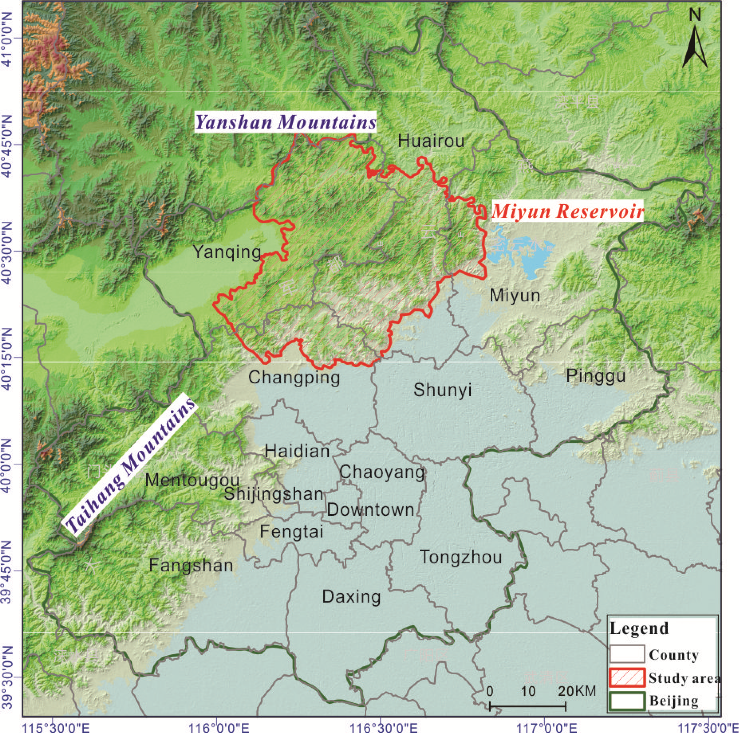
2.1. Study Area

The study area is located in the north of Jundushan Mountain, in Beijing, consisting of north of Changpin County, northeast of Yanqing County, mid-south of Huairou County, and west of Miyun County (Figure 1). The altitude is 587 m on average, ranging from 182 m to 1503 m, and the maximum and mean slope calculated from DEM (Digital Elevation Model) are 76.2° and 22.8°. The climate belongs to the temperate semi-humid continental monsoon climate, where the annual average temperature is about 2–11 °C and the mean annual precipitation is 450–660 mm depending on the altitude. Shrubs are widely distributed in this area. Moreover, deciduous broadleaved forest and temperate coniferous forest are the dominant types of forest vegetation in this area, such as Quercus, Tilia, Fraxinus, Acer, Populus, Pinus tabulaeformis, and Biota orientalis. The main shrub types are Vitex negundo, Spiraea trilobata, Myripnois dioica, and Deutzia grandiflora. In this area, dominant species distribution are usually mixed, for example, Vitex negundo mixes with wild Jujube, Vitex negundo mixes with Spiraea trilobata and Prunus armeniaca, Vitex negundo mixes with Spiraea trilobata and Myripnois dioica, etc.

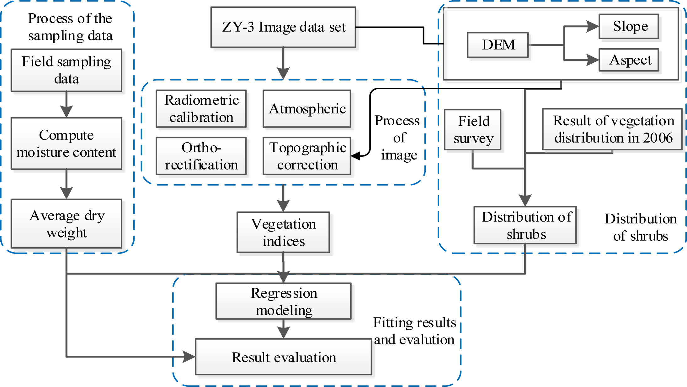
2.2. Data Acquisition and Processing

2.2.1. Satellite Image Data and DEM

The ZY-3 image was acquired on 22 August 2012. The solar zenith angle is 29.58° and the solar azimuth angle is 147.80°. The ZY-3 satellite operates in a sun-synchronous round orbit at an altitude of 506 km, with a global coverage every 3–5 days. Four cameras are carried on the ZY-3 platform, namely a 2.1 m resolution nadir looking panchromatic TDI (Time Delay Integration) CCD camera, a pair of 3.5 m resolution front and backward looking panchromatic CCD cameras and one 5.8 m resolution nadir looking multi-spectral CCD camera. The multi-spectral camera has 4 bands—Blue (0.45–0.52 μm), Green (0.52–0.59 μm), Red (0.63–0.69 μm), and Near-infrared (0.77–0.89 μm).
Compared with other resources satellites launched by China, ZY-3 has higher spatial resolution, higher geometric accuracy as well as better positioning accuracy. In addition, it has tilt capability and stereo mapping capability at 1:50,000 scale. The experiments in this research suggested that a DSM (Digital Surface Model) could be extracted from the front and back view of high-resolution panchromatic data. Through geometric correction with a 1:50,000 relief map and resampling a DEM could be produced at a spatial resolution of 10 m.

2.2.2. Field Sampling Data

The field investigation is part of the “National Remote Sensing Investigation and Evaluation of the Ecological Environmental Changes in Ten Years” starting in June 2012. During three months, 1206 points were checked and more than 300 samples were collected, which covered all over Beijing and concentrated in the northern mountains. And the field investigation in the study area was carried out in August. According to the geographical distribution of the shrub and the area characteristics, altitude and shrub types, thirty 100 m × 100 m sample plots were set up, and from each plot three 30 m × 30 m regions were set, in which three 10 m × 10 m small squares were used. Due to the limits of the terrain and weather condition, we acquired 84 effective group samples in all of 90 sample regions.
For each square, the geographical measurements including the No. of the square, the GPS coordinate in the center of the square, altitude, slope, and aspect were recorded. Species and canopy measurements within the square were also recorded including the name and count of dominant species, the fresh weight, the plant height, as well as the density, and the LAI (Leaf Area Index) value, and fisheye photos were taken. We fetched 100 g samples from every sample region into numbered bags and dried them under constant temperate in the laboratory and computed values of moisture content according to Equation (1), translated fresh weight to dry weight and recorded it. The average dry biomass per unit area (1 m × 1 m) in the sample area was recorded (unit is g/m2).
W i = 1 3 j = 1 3 ( w ij × n ij 100 × ( 1 μ i ) ) i = 1 , 2 , , 72 ; j = 1 , 2 , 3 ;
where: wij= fresh weight of the jth quadrat; nij = plant count of the jth quadrat; μi = moisture content of the ith area; Wi = dry biomass of per unit area in the ith area.

2.2.3. Data Processing

There are three steps to process the satellite image: radiometric calibration, geometric correction, and atmospheric correction. The parameters for conversion of digital numbers (DN) to radiance (W·m−2·sr−1·μm−1) were provided by the Satellite Surveying and Mapping Application Center, NASG, as well as the solar azimuth angle and the solar zenith angle. Atmospheric correction was based on the FLAASH (Fast Line-of-sight Atmospheric Analysis of Spectral Hypercubes) algorithm, and the radiance (μW·cm−2·nm−1·sr−1) was converted to surface reflectance. The parameters used for the atmospheric correction are listed in Table 1. The RPC (Rational Polynomial Cofficients) file and ground control points were used to implement ortho-rectification, in which the error was limited to 0.5 pixels. Finally, the study area was extracted from the image, and the slope and aspect data were extracted from DEM data by modeling.
In order to ensure the effectiveness of the fitting result and the accuracy of the assessment result, the sample data was classified through a stratified sampling method according to the altitude. Seventy-two groups of sample data were used to build the biomass model, and the remaining 12 groups were used to assess the model accuracy.

2.3. Methods

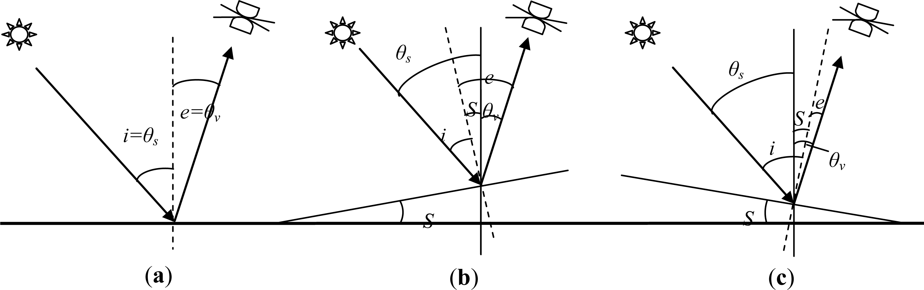
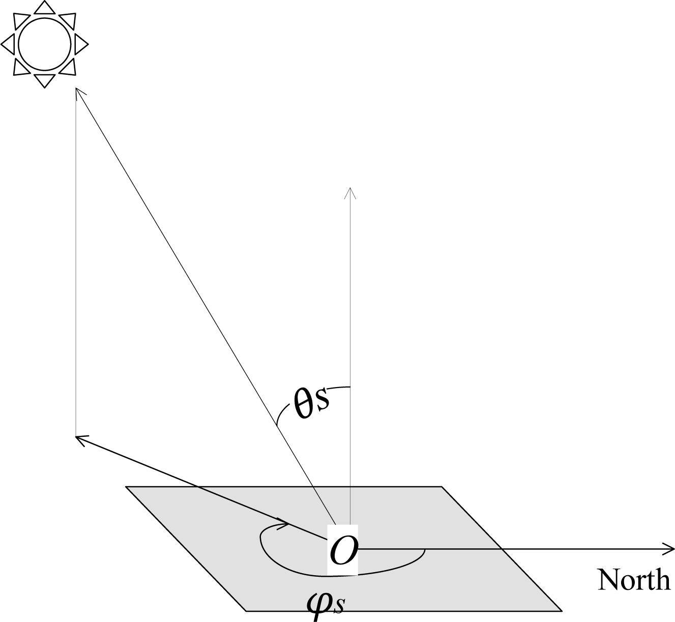
2.3.1. Topographic Correction Models

Currently, four types of topographic correction models are mainly used based on DEM: empirical-statistical models [7,17], normalization models [18], Lambertian reflection models [19] and non-Lambertian reflection models [11,20]. Some common Lambertian and non-Lambertian reflection models are presented in Table 2. Law and Nichol’s study [21] shows that all methods can be applied to surface reflectance (after atmospheric correction in this paper) or the apparent or top-of-atmosphere (TOA) reflectance.
Table 2. The topographic correction models used in this study.
Topographic Correction ModelsExpressionPresenterTransformation Expression
1Cosine L m = L ( cos θ s / cos i )Teillet [7] ρ h = ρ ( cos θ s / cos i )
2C-HuangWei L m = ( L L min ) ( cos θ s cosi min cosi cosi min ) + L minHuangWei et al. [9] ρ h = ( ρ ρ min ) ( cos θ s cosi min cosi cosi min ) + ρ min
3SCS+C L m = L ( cos θ s cos S + C cosi + C )Soenen et al. [11] ρ h = ρ ( cos θ s cos S + C cosi + C )
4Minnaert L m = L ( cose cos k i cos k e )Smith et al. [12] ρ h = ρ ( cose cos k i cos k e )
5Minnaert+SCS L m = L ( cos k θ s cos S cos k i )Reeder [13] ρ h = ρ ( cos k θ s cos S cos k i )
where: Lm = radiance after correction; L = radiance before correction; Lmin = minimum radiance before correction; ρh = reflectance of a horizontal surface; ρ = reflectance of an inclined terrain; ρmin = minimum reflectance of an inclined terrain; θs = solar zenith angle; S = slope; i = solar incident angle (Figure 2); e = angle of incidence for the receiving sensor, and in this paper, the e value is equal to S due to the satellite angle of tilt (θv equals to 0 in Figure 2); θv = sensor incident angle; C = empirical constant; k = Minnaert constant.
The cosi can be expressed as:
cosi = cos θ s cosS + sin θ s sinScos ( φ s A )
where: ϕs = solar azimuth angle (measured in Figure 3); A = aspect.
In the C correction model and the SCS+C model, the C can be calculated based on the linear relationship between the original reflectance and the cosine of the solar incident angle (Equation (3)).
ρ = a + bcosi
where: ρ = reflectance of pixels before topographical correction; a = intercept of the linear fitting result; b = slope of the linear fitting result; where a represents the intercept of the linear expression while b is the slope of the linear expression. C can be calculated by fitting the result of a and b, which is expressed as: C = a/b.
Previous research suggested that the Minnaert model based on the non-Lambertian reflectance assumption performed better than other topographical correction models [22]. It overcomes shortcomings of Lambertian reflection models by adjusting the magnitude of the topographic correction through considering the empirical constant k, which has been tuned to fit the observed BRDF, and was introduced by Minnaert in 1941. The k value ranges from 0 to 1 according to the surface of the object. If the surface is Lambertian, k is equal to 1, otherwise k is less than 1. In addition, the value of k depends on both the type of land cover and the image band, and is computed by the conventional regression fitting linear equation.
The Minnaert model expression in Table 2 can be written as below:
L m ( cos k i cos k e ) = L cose
Taking the logarithm on both sides, Equation (4) can be written as:
ln L m + k ln ( cosi cose ) = ln ( L cose )
Consider x = ln(cosi × cose), y = ln(L × cose), m = lnLm, then we propose the linear representation of Equation (5) as:
y = kx + m
Note that the sample points used for regression fitting must be selected from the same type of land cover and then we can compute the value of x and y of every sample. For the sample pixel, both k and m are constants, and k can be computed by linear fitting.
The parameters of each model were calculated before performing the topographic correction, 5000 vegetation sample points are created randomly in each remote sensing image. C and k of each image band can be linear fitted by Equations (3) and (5). In this paper, the authors selected the 5 common topographical correction models listed in Table 2. Then the values of all constants for each band are listed in Table 3.

2.3.2. Biomass Estimation

Previous research suggested that a correlation exists between dry biomass of vegetation in the growth state vegetation and various vegetation indices [2327], and it is important to consider overall multiple vegetation index combinations to estimate the biomass.
Considering the distribution and plant architecture of shrub community characteristics, and the fact that the vegetation indices are sensitive to the soil environment, we tested ten vegetation indices, including NDVI (Normalized Difference Vegetation Index) [28], MSAVI (Modified Soil Adjusted Vegetation Index) [29], GNDVI (Green Normalized Difference Vegetation Index) [30], MTVI2 (Modified Triangular Vegetation Index 2) [31], MSR (Modified Simple Ratio Vegetation Index) [32], RDVI (Ratio Difference Vegetation Index) [33], IPVI (Infrared Percentage Vegetation Index) [34], OSAVI (Optimized Soil Adjusted Vegetation Index) [35], NLI (Non-Linear Index) [36], and TVI (Triangular Vegetation Index) [37], listed in Table 4 to fit the estimation models.
Figure 4 is the workflow for biomass estimation. There are five parts in the flow: remote sensing data preprocessing and vegetation index extraction; Vitex negundo extraction; field data sampling processing; model fitting and accuracy assessment and biomass distribution mapping. The remote sensing data preprocessing includes radiometric calibration, atmospheric correction, geometric correction, image clipping and the extraction of ten vegetation indices. Then, drawing the map of the shrubs’ distribution in the study area, by using the vegetation distribution map of Beijing in 2006, DEM data, slope data, aspect data and the shrub field survey results. Finally, estimating Vitex negundo vegetation indices and its canopy biomass fitting models by the least squares method and evaluating the models’ accuracy to select the optimal one. In the selected process, remote sensing data preprocessing, topographical correction by the Minnaert+SCS model, vegetation indices extraction and biomass estimation by the least squares method are in the process, respectively.

3. Result

3.1. Comparison of Different Topographic Correction Models

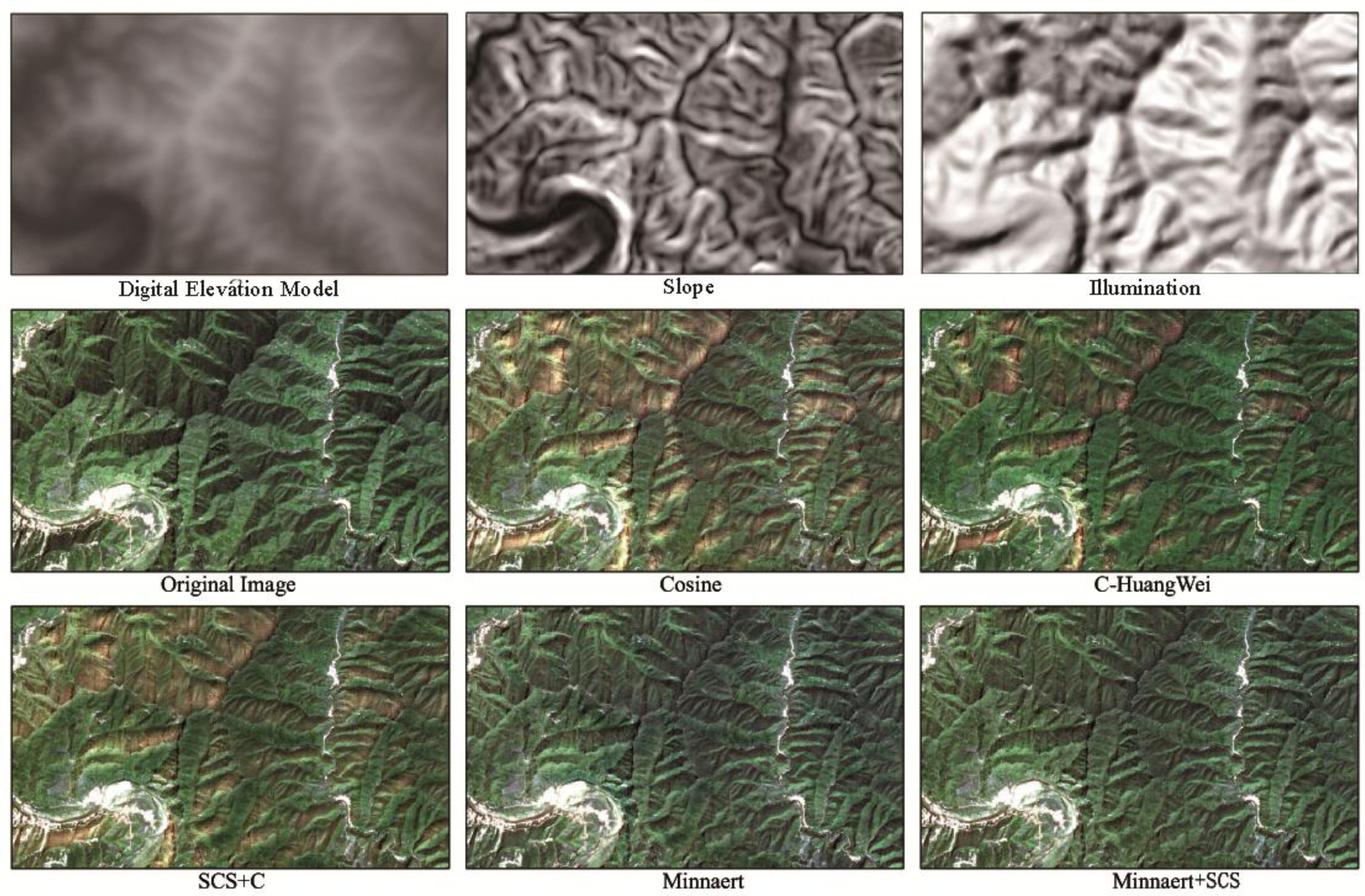
3.1.1. Visual Inspection

Figure 5 displays a sub-scene of the ZY-3 scene. The true color composite ZY-3 bands 3, 2, and 1 as red, green, and blue for a small mountainous area in the study area is illustrated to highlight the difference before and after topographic corrections. Elevations range from 100 m to 1182 m, slopes between 0° and 41°. The illumination (cosi) represents the cosine of the solar incident angle. Bright areas receive a higher illumination, while dark areas have a lower one. The comparison between the images showed that all topographic correction methods minimized the topographic effect by minimizing the three-dimensional impressions in the topographically normalized images. However, the Minnaert and Minnaert+SCS corrections seemed to show a greater decrease in the three-dimensional relief effect. While the Cosine, C-HuangWei and the SCS+C corrections showed similar visual effect, and obviously over-correction appeared after correction, which is mainly caused by the defects of the Lambertian reflectance assumption.

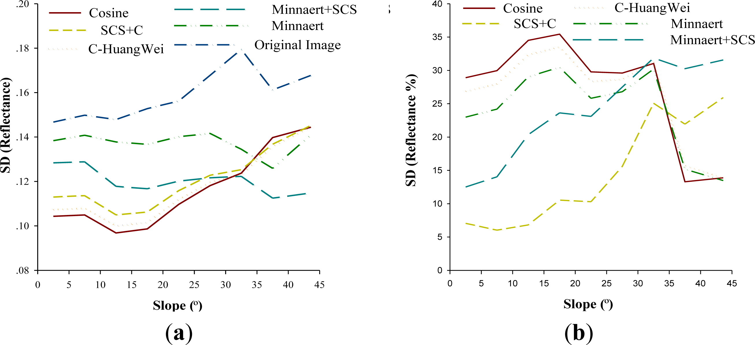
3.1.2. Statistical Analysis

The mean reduction (%) in SD for vegetation pixels after correction is presented in Table 5. These are the values for the 5000 vegetation sample points (mentioned in the calculation of the correction parameters before) used for our assessment, taken under a range of slope angles (from 0° to 43.6°). The SD should decrease after a successful shade removal, meaning that the impact of illumination is reduced [14].
First it can be seen from the table that the simpler methods based on the Lambertian reflectance assumption, such as the Cosine correction and the C-HuangWei correction, reduce in general the SD but in a rather limited way, giving clearly higher SD than some of the other methods. Second, it can be observed that the Minnaert and Minnaert+SCS corrections generate lower SD than the other methods. Moreover, all the methods cannot reduce the SD of all bands simultaneously.
In Figure 6a, we can see that the regression lines can be divided into three groups according to the variation tendency of the SD with the increase of the slope. The SD for the original image rises steadily from 0° to 7.5°. There is then a slight fluctuation for an increase until to 23°. After rising more sharply for the next 10°, there is a moderate dip, followed by a gradual rise until 43.6°. It is projected to peak at 0.18 at around 33°. In addition, lines representing the Cosine correction, C-HuangWei correction, and the SCS+C correction show a general upward trend with the increase of the slope angle, as well as the line stands for the original image. This group of lines offer similar results, with similar SD for the fourth band of the ZY-3 image with a slope angle > 33°, and reaches a peak at 0.145 at 43.6°. However, the Minnaert correction and the Minnaert+SCS correction fluctuate for a slight dip until 37°, followed by a rise until 43.6°. Figure 6b shows the distribution of the mean reduction (%) of SD (for the fourth band) for different slope angles. As can be seen from the illustration, the group of Lambertian corrections fluctuates until to 33°, there is a sharp dip to 13 percent at 37.5°. The group of the non-Lambertian corrections shows general rise until 37.5°, and reaches the peak at around 37.5°. There is then a steadily drop for the Minneart+SCS correction, followed by a slight rise until 43.6°. It can be concluded from Figure 6 that the non-Lamertain corrections perform better than the group of Lambertian correction under high slope angles (>33°). The analysis performed for the images shows that the best results were obtained by the non-Lambertian corrections including the Minnaert method and the Minnaert+SCS method. To a lesser extent, as can be seen from Table 5, the SCS+C correction gives good results as well.

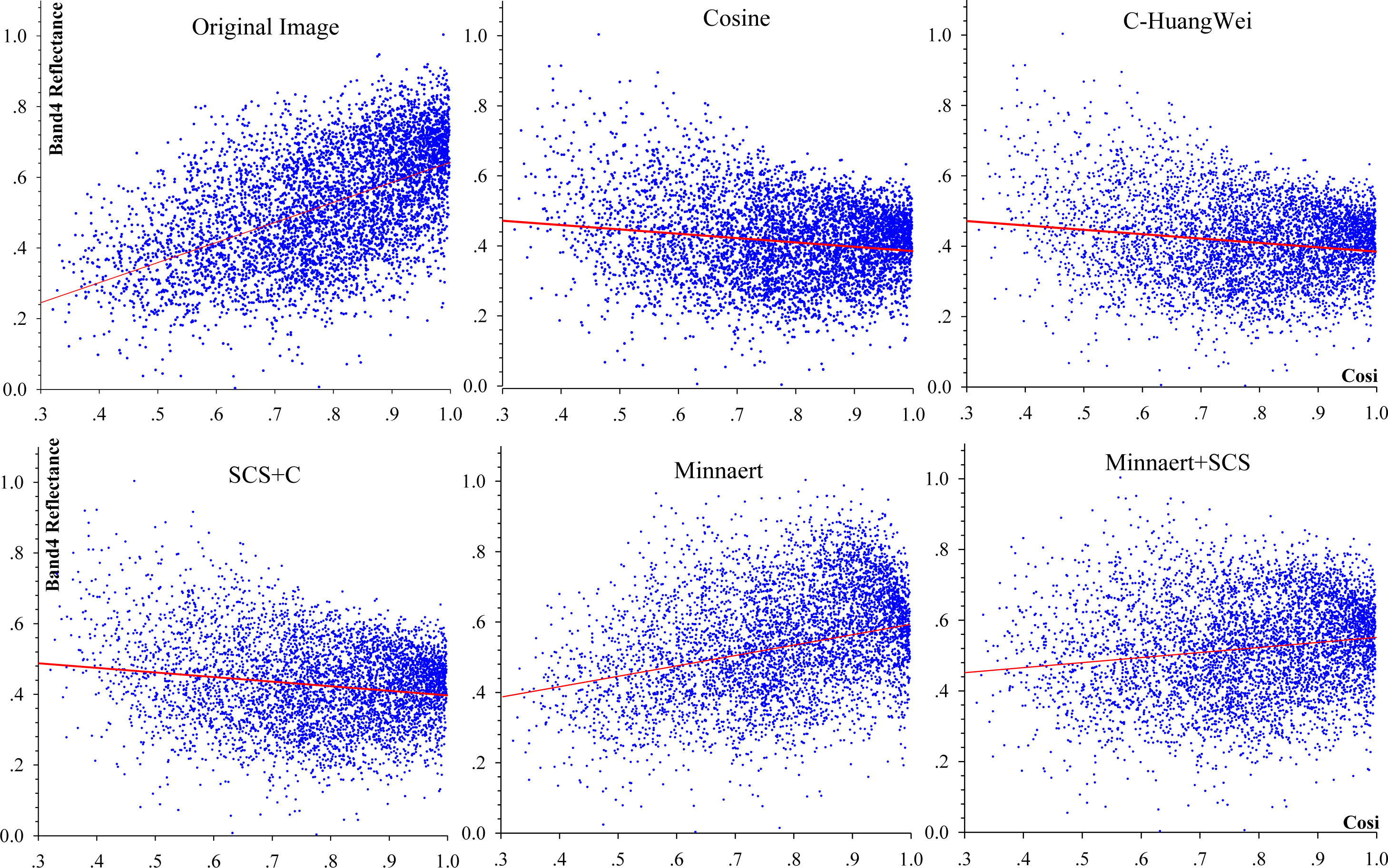
3.1.3. Correlation Analysis

Previous studies show that the pixel reflectance of image data in regions of large relief has obviously correlation with the cosine of the solar incident angle, and the correlation obviously weakened or even vanished after terrain correction [11,38]. Theoretically, a greater slope absolute value of linear fitting expressions between the pixel reflectance and cosine indicates a more obvious terrain effect; in addition the greater the correlation coefficient R2, the more obvious the terrain effects. Band 4, for example, by taking 5000 sample points randomly from the image before and after correction respectively, a scatter diagram (Figure 7) is shown below, the coordinate axis respectively represents pixel reflectance and the cosine of the solar incident angle value of the fourth band.
As we can see from the diagram, for the original image, the scatter distribution and the regression fitting line of reflectance and cosi are in the tilt state obviously, while the tilt decreased significantly after correction. Thus, it is obvious that all correction models can weaken the terrain effect in a certain degree in this study. For the Cosine model, C-HuangWei and SCS+C model, regression-fitting lines incline in the opposite direction against the original image, due to excessive correction. In contrast, the scatter distribution and the fitting line tilt of the Minnaert decreased significantly, as well as that of the Minnaert+SCS, which has a horizontal trend. Furthermore, it indicates that the effect of Minnaert+SCS is preferable to that of Minnaert and the rest of the three models. The pixel reflectance and cosi fitting results of band4 from different correction results are shown in Table 6. Similarly, the original image has the higher correlation coefficient (R2 reaches 0.306) and gradient of the fitting line, while the Minnaert+SCS result has the lowest in both. Besides, the results of Cosine, C-HuangWei and SCS+C have a negative correlation with cosi. In a word, the comparison and analysis show that Minnaert+SCS correction performs better than other models in this paper.

3.2. Effects on Biomass Estimation

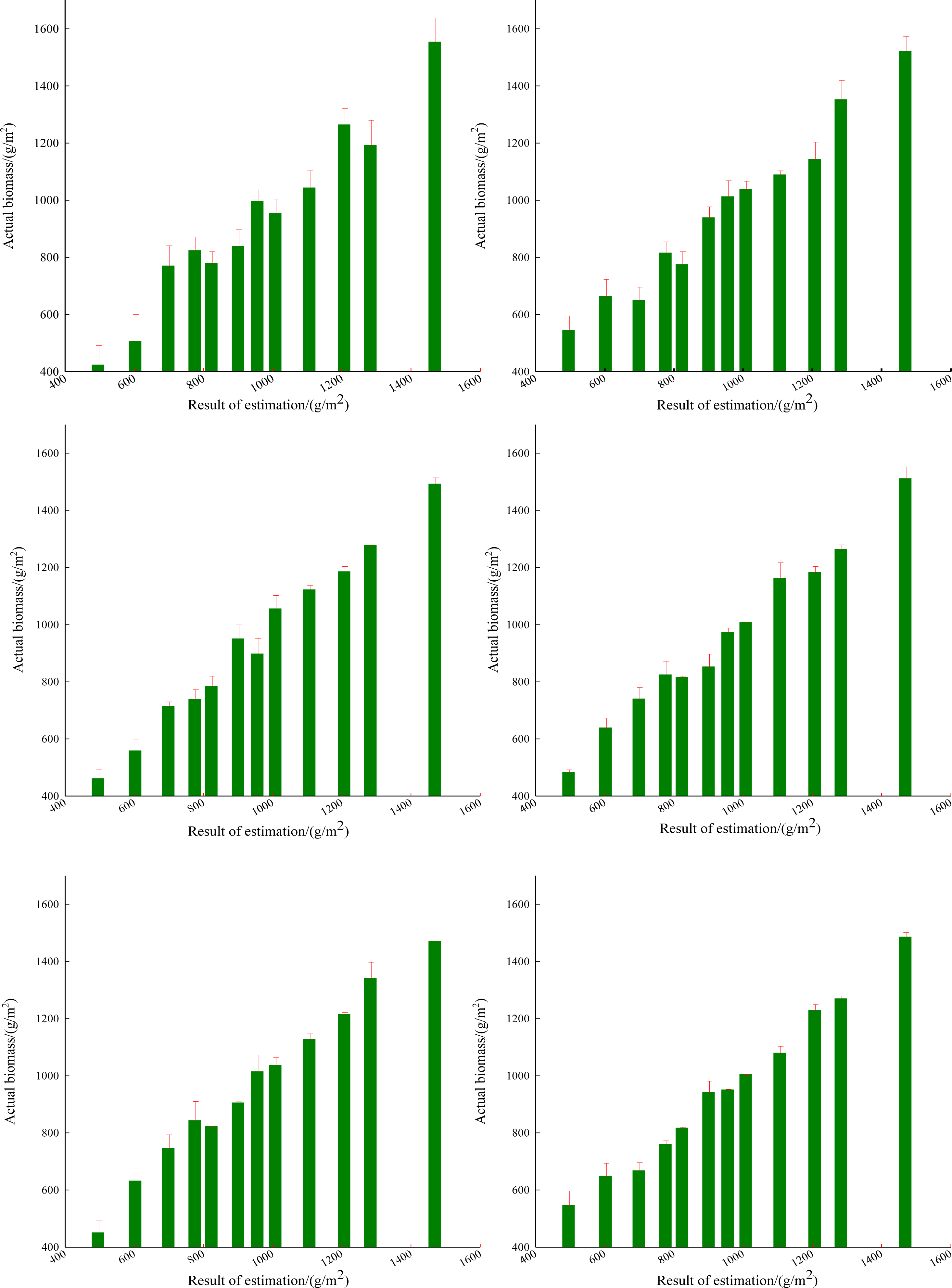
3.2.1. Fitting Results of Biomass

In this paper, we used the regression analysis method to fit leaf biomass of shrub in the Beijing mountain area, and solved the parameters by the least square method. Due to the abnormal distribution of the sample data, the Kendall correlation coefficient was used in the correlation analysis between the 10 groups of vegetation indices and biomass sample data (in IBM SPSS Statistic software, version 20.0). Results showed that the NDVI, OSAVI, MTVI2, GNDVI, NLI, MSAVI, RDVI, and IPVI had significant correlation with the biomass data, while the correlation between TVI or MSR with the biomass was not so significant; NDVI, MSAVI, GNDVI, MTVI2, MSR, RDVI, and IPVI had a non-ignorable correlation with OSAVI; Furthermore, there were significant linear relationships between MSAVI and other vegetation indices. In order to ensure the sample variables are independent and have low correlation with each other, the authors removed vegetation indices that had correlation with others, such as NDVI, OSAVI, and MSAVI, and chose TVI, MTVI2, GNDVI, NLI, MSR, RDVI, and IPVI (the latter fails to pass the correlation test during the regression and is therefore removed) to fit biomass by the regression method. We then got the fitting results of different terrain corrections (Table 7).
From Table 7, the determination coefficient R2 reaches more than 0.75, and the model significance is significant (p < 0.05), which shows that the fitting models have good robustness, and they can express the arithmetical relationship between vegetation indices and leaf biomass. For the three types of Lambertian reflection corrections, the R2 of the fitting equation increased compared to the original image data, but still stayed below 0.8, and have reached a significant level (p < 0.05). For the non-Lambertian reflection correction, Minnaert and Minnaert + SCS, the R2 of the fitting equation after correction reached more than 0.85, and have reached a more meaningful level (p < 0.01). Furthermore, the fitting result of Minnaert+SCS correction had higher R2 and precision, which increased by 0.113 and 15.8 g/m2, respectively, in contrast to the original image.

3.2.2. Effects on Biomass Estimation

In this section, the authors used the fitting results above for biomass estimation, and the residue between estimation results and the measured biomass of the 12 samples is shown in Figure 8. At first glance, the distribution of sample bars in every diagram is near the 1:1 contour, which shows that the biomass estimation fitting results are reliable. Furthermore, for the original image, inversion results with the measured SD of 74.1 g/m2, and the statistics maximum error reaches 99.6 g/m2, for which there are three main causes: first of all, the shrubs have special distribution characteristics and plant structure, mostly forested, and uneven distribution on sunny slopes more than in shade; Second, the discontinuity of sampling and too much rain in August in the Beijing mountain area, in 2012, contributed to vegetation grown apace, caused a deviation of the sample data. Third, due to the geometric deformation caused by the ZY-3 satellite observation angle to a certain extent, in the mountain area. In addition, the determination of regression parameters in the topographic correction model is also the principal factor that affects the final result. As mentioned above, the Cosine, C-HuangWei and SCS+C correction resulted in greater error in the regions where the biomass is higher or lower, and the maximum error reached 100.2 g/m2; as a result of excessive correction in slope pixels. However, for the Minnaert model and the Minnaert+SCS model, being based on the assumption of the non-Lambertian reflection, showed stable characteristics, where the error range is controlled within the 85 g/m2. Especially for the Minnaert+SCS correction result, where the SD reaches 58.4 g/m2, with the maximum error of 64.7 g/m2 (Table 8). Besides, overcorrection results seem to be much better than the uncorrected image, as can be seen from the statistics result in Tables 7 and 8.

4. Discussion

For quantitative estimation based on remote sensing reflectance and vegetation indices, the precision of the inversion model largely depends on the remote sensing data processing, and the determination of the parameters in the process of modeling. In addition, parameter selection is extremely important. On the extent of the study area, the k value is a constant, while during the process of calculation, it can be found that the k partially depends on the geometric parameters such as the solar incident angle and slope. Lu et al. [39] found that there was a non-ignorable deviation between the fitting values of k under different slope grade, which showed that the correction precision of a large region of relief need to be further improved.
In this paper, the DEM data used were processed from the stereopair of the ZY-3 images, which consisted of forward and backward looking panchromatic images with a resolution of 10 m. However, it is clear that the resolution of the DEM is inconsistent with that of the remote sensing data, so that re-sampling in the process of data processing hardly can be avoided, therefore, it is bound to affect the precision of the topographic correction. Nevertheless, there is no definite conclusion at present about the best matching combination between the resolution of the DEM and that of the original image [40]. In addition, the selection of the random sample points has a crucial impact on the calculation results of the topographic correction model regression parameters (such as k and C), such that different sets of sample points will result in different regression parameters. Therefore a method to confirm the regression parameters more scientifically is still needed. In addition, the terrain ups and downs are often associated with the change of the vertical distribution of vegetation, such as the difference of vegetation in different slope angles and different elevation level, and different growth status of the same vegetation. Therefore, whether the original image pixel brightness (or reflectance) change is caused by topographic relief or characteristic spectral features itself, should be taken into consideration in the improvement of the topographic correction method.
In practical, scenes with different zenith angles should better be investigated to evaluate the performance of a topographic correction method [14,41]. However, studies of previous researchers were sufficient to verify the validity of the corrections resulted from different solar zenith angles. With respect to this reality, like many researchers [5,22,39], we did not examine the correction effects under different illumination criteria in this paper. Thus, it can also be concluded from the previous researches’ studies that methods such as Minnaert, based on Non-Lambertain models, have better performance under lower solar zenith angle [14]. While they may have performed the worst [5] under a large solar zenith angle about 65°.
In addition, the regression model for biomass estimation is only suitable for the time and environmental conditions in the study area, as well as the processing method of the field sampling data. In different seasons and different geographical conditions, the biomass fitting models show obvious differences [27]. For the discontinuous distribution and the special plant architecture of the shrubs, the pixels in the image data are affected by the soil background easily. Moreover, due to the resistance to cold and drought, shrubs also distribute in the high altitude and infertile localities, where the reflectance of the canopy is easily affected by the background of soil and rock. Therefore, in the future research we will investigate how to improve the typicality of sampling and the universality of the inversion model.

5. Conclusions

In this paper, we compared five commonly-used topographic correction models on the ZY-3 satellite multispectral images, then discussed the impacts of different models on shrub biomass estimation over Beijing Jundushan Mountain. From the results, we drew the following conclusions:
(1)
The topographic correction model based on Lambertian reflection theory tends to cause excessive correction due to the sky diffuse reflection and the surrounding terrain. The models based on non-Lambertian reflection assumption yield better correction results. Visual comparison, statistical analysis and correlation analysis show that the Minnaert+SCS model can effectively weaken the influence of terrain relief on pixels in ZY-3 satellite multispectral images, and restore a true reflectance of the pixels in the relief area.
(2)
The precision of the regression fitting between spectral vegetation indices and shrub leaf biomass is improved after topographic correction, as well as the determination coefficient R2. All the above shows that the topographic correction on ZY-3 satellite data is able to improve the estimation of shrub leaf biomass to a certain extent. In addition, results based on non-Lambertian reflection models are superior to those based on Lambertian reflection models. Furthermore, with the Minnaert+SCS model, the biomass regression fitting result has the R2 of 0.869, and the SD is reduced to 58.4 g/m2, which suggests that in areas of topographic relief, topographic correction is indispensable to the biomass estimation based on vegetation indices.
(3)
Further research should be carried out with imagery acquired from different sensors and solar zenith angles, to examine the performances of the methods under different illumination criteria. Moreover, how the accuracy of the DEM affects the results of topographic correction of ZY-3 imagery should also be investigated in future studies.
In this paper, the authors make full use of the domestically made satellite products of China, in order to show its potential ability to the remotely sensed quantitative research.

Acknowledgments

This research was financially supported by the National Natural Science Foundation of China (General Program, Grant No. 41101404; Key Program, Grant No. 41130744; General Program, Grant No. 41171335) and the International Science & Technology Cooperation Program of China (Grant No. 2014DFA21620). Thanks Prof. Dong Hu for the guidance on the field work. The ZY-3 satellite data and related parameters are provided by Satellite Surveying and Mapping Application Center, NASG.

Author Contributions

Ming-Liang Gao, Wen-Ji Zhao and Zhao-Ning Gong conceived and designed the study. Ming-Liang Gao, Wen-Ji Zhao, Zhao-Ning Gong, Hui-Li Gong and Zheng Chen performed the experiments. Xin-Ming Tang provided the images. Ming-Liang Gao and Zheng Chen wrote the paper. Ming-Liang Gao, Wen-Ji Zhao, Zhao-Ning Gong, Hui-Li Gong and Zheng Chen reviewed and edited the manuscript. All authors read and approved the manuscript.

Conflicts of Interest

The authors declare no conflict of interest.

References

  1. Du, N.; Zhang, X.R.; Wang, W.; Chen, H.; Tan, X.F.; Wang, R.Q.; Guo, W.H. Foliar phenotypic plasticity of a warm-temperate shrub, vitex negundo var. heterophylla, to different light environments in the field. Acta Ecol. Sin 2011, 31, 6049–6059. (In Chinese) [Google Scholar]
  2. Yin, Z.F.; Ouyang, H.; Xu, X.L.; Song, M.H.; Duan, D.Y.; Zhang, X.Z. Water and heat balance and water use of shrub grassland and crop fields in Lhasa River Valley. Acta Geogr. Sin 2009, 64, 303–314. (In Chinese) [Google Scholar]
  3. Estornell, J.; Ruiz, L.A.; Velázquez-Martí, B.; Hermosilla, T. Estimation of biomass and volume of shrub vegetation using LiDAR and spectral data in a Mediterranean environment. Biomass Bioenergy 2012, 46, 710–721. [Google Scholar]
  4. Estornell, J.; Ruiz, L.A.; Velázquez-Martí, B.; Fernández-Sarría, A. Estimation of shrub biomass by airborne LiDAR data in small forest stands. For. Ecol. Manag 2011, 262, 1697–1703. [Google Scholar]
  5. Gao, Y.N.; Zhang, W.C. A simple empirical topographic correction method for ETM+ imagery. Int. J. Remote Sens 2009, 30, 2259–2275. [Google Scholar]
  6. Gao, Y.N.; Zhang, W.C. Comparison test and research progress of topographic correction on remotely sensed data. Geogr. Res 2008, 27, 467–477. [Google Scholar]
  7. Teillet, P.M.; Guindon, B.; Goodenough, D.G. On the slope-aspect correction of multispectral scanner data. Can. J. Remote Sens 1982, 8, 84–106. [Google Scholar]
  8. Gao, Y.N.; Zhang, W.C. Simplification and modification of a physical topographic correction algorithm for remotely sensed data. Acta Geodaet. Cartogr. Sin 2008, 37, 89–94. (In Chinese) [Google Scholar]
  9. Huang, W.; Zhang, L.P.; Li, P.X. An improved topographic correction approach for satellite image. J. Image Graph 2005, 10, 1124–1128. [Google Scholar]
  10. Gu, D.; Gillespie, A. Topographic normalization of landsat TM images of forest based on subpixel Sun-Canopy-Sensor geometry. Remote Sens. Environ 1998, 64, 166–175. [Google Scholar]
  11. Soenen, S.A.; Peddle, D.R.; Coburn, C.A. SCS+C: A modified Sun-Canopy-Sensor topographic correction in forested terrain. IEEE Trans. Geosci. Remote Sens 2005, 43, 2148–2159. [Google Scholar]
  12. Smith, J.A.; Lin, T.L.; Ranson, K.J. The Lambertian assumption and Landsat data. Photogramm. Eng. Remote Sens 1980, 46, 1183–1189. [Google Scholar]
  13. Reeder, D.H. Topographic Correction of Satellite Images: Theory and Application; Dartmouth College: Hanover, NH, USA, 2002. [Google Scholar]
  14. Stijn, H.; Emilio, C. Evaluation of different topographic correction methods for Landsat imagery. Int. J. Appl. Earth Observ. Geoinf 2011, 13, 691–700. [Google Scholar]
  15. Shi, D.; Yan, G.J.; Mu, X.H. Optical remote sensing image apparent radiance topographic correction physical model. J. Remote Sens 2009, 6, 1030–1046. [Google Scholar]
  16. Ediriweera, S.; Pathirana, S.; Danaher, T.; Nichols, D.; Moffiet, T. Evaluation of different topographic corrections for Landsat TM data by prediction of foliage projective cover (FPC) in topographically complex landscapes. Remote Sens 2013, 5, 6767–6789. [Google Scholar]
  17. Vincini, M.; Reeder, D.; Frazzi, E. An Empirical Topographic Normalization Method for Forest TM Data. In Proceedings of the 2002 IEEE International Geoscience and Remote Sensing Symposium (IGARSS), Toronto, Canada, 24–28 June 2002; Volume 4, pp. 2091–2093.
  18. Civco, D.L. Topographic normalization of Landsat thematic mapper digital magery. Photogram. Eng. Remote Sens 1989, 55, 1303–1309. [Google Scholar]
  19. Dymond, J.R.; Shepherd, J.D. Correction of the topographic effect in remote sensing. IEEE Trans. Geosci. Remote Sens 1999, 37, 2618–2620. [Google Scholar]
  20. Ekstrand, S. Landsat TM-based forest damage assessment: Correction for topographic effects. Photogram. Eng. Remote Sens 1996, 62, 51–161. [Google Scholar]
  21. Richter, R.; Kellenberger, T.; Kaufmann, H. Comparison of topographic correction methods. Remote Sens 2009, 1, 184–196. [Google Scholar]
  22. Law, K.H.; Nichol, J. Topographic Correction for Differential Illumination Effects on IKONOS Satellite Imagery. In Proceedings of the 10th Congress of International Society for Photogrammetry and Remote Sensing, Istanbul, Turkey, 12–23 July 2004; Volume 35, p. 6.
  23. Gao, M.L.; Zhao, W.J.; Gong, Z.N.; He, X.H. The study of vegetation biomass inversion based on the HJ satellite data in Yellow River wetland. Acta Ecol. Sin 2013, 33, 542–553. (In Chinese) [Google Scholar]
  24. Li, X.; Yeh, A.; Liu, K.; Wang, S.G. Inventory of mangrove wetlands in the Pearl River Estuary of China using remote sensing. J. Geogr. Sci 2006, 16, 155–164. [Google Scholar]
  25. Li, S.; Zhang, Z.L.; Zhou, D.M. An estimation of aboveground vegetation biomass in a national natural reserve using remote sensing. Acta Ecol. Sin 2011, 30, 278–290. [Google Scholar]
  26. Guo, Z.F.; Chi, H.; Sun, G.Q. Estimating forest aboveground biomass using HJ-1 Satellite CCD and ICESat GLAS waveform data. Sci. China: Earth Sci 2010, 53, 16–25. [Google Scholar]
  27. Anaya, J.A.; Chuvieco, E.; Palacios-Orueta, A. Aboveground biomass assessment in Colombia: A remote sensing approach. For. Ecol. Manag 2009, 257, 1237–1246. [Google Scholar]
  28. Deering, D.W.; Haas, R.H.; Rouse, J.W.; Schell, J.A. Monitoring the Vernal Advancement of Retrogradation of Natural Vegetation; Final Report 1974; NASA/GSFC: Greenbelt, MD, USA, 1974. [Google Scholar]
  29. Qi, J.; Chehbouni, A.; Huete, A.R.; Kerr, Y.H.; Sorooshian, S. A modified soil adjusted vegetation index. Remote Sens. Environ 1994, 48, 119–126. [Google Scholar]
  30. Gitelson, A.A.; Kaufman, Y.J.; Merzlyak, M.N. Use of a green channel in remote sensing of global vegetation from EOS-MODIS. Remote Sens. Environ 1996, 58, 289–298. [Google Scholar]
  31. Haboudane, D.; Miller, J.R.; Pattey, E.; Zarco-Tejada, P.J.; Strachan, I.B. Hyperspectral vegetation indices and novel algorithms for predicting green LAI of crop canopies: Modeling and validation in the context of precision agriculture. Remote Sens. Environ 2004, 90, 337–352. [Google Scholar]
  32. Chen, J. Evaluation of vegetation indices and a modified simple ratio for boreal applications. Can. J. Remote Sens 1996, 22, 229–242. [Google Scholar]
  33. Roujean, J.L.; Breon, F.M. Estimating PAR absorbed by vegetation from bidirectional reflectance measurements. Remote Sens. Environ 1995, 51, 375–384. [Google Scholar]
  34. Crippen, R.E. Calculating the vegetation index faster. Remote Sens. Environ 1990, 34, 71–73. [Google Scholar]
  35. Rondeaux, G.; Steven, M.; Baret, F. Optimization of soil-adjusted vegetation indices. Remote Sens. Environ 1996, 55, 95–107. [Google Scholar]
  36. Goel, N.S.; Qin, W.H. Influences of canopy architecture on relationships between various vegetation indices and LAI and FPAR: A computer simulation. Remote Sens. Rev 1994, 10, 309–347. [Google Scholar]
  37. Broge, N.H.; Leblanc, E. Comparing prediction power and stability of broadband and hyperspectral vegetation indices for estimation of green leaf area index and canopy chlorophyll density. Remote Sens. Environ 2000, 76, 156–172. [Google Scholar]
  38. Holben, B.N.; Justice, C.O. The topographic effect on spectral response from Nadir-Pointing sensors. Photogram. Eng. Remote Sens 1980, 46, 1191–1200. [Google Scholar]
  39. Lu, D.S.; Ge, H.; He, S.Z.; Xu, A.J.; Zhou, G.M.; Du, H.Q. Pixel-based Minnaert correction method for reducing topographic effects on a Landsat 7 ETM+ image. Photogram. Eng. Remote Sens 2008, 74, 1343–1350. [Google Scholar]
  40. Conese, C.; Gilabert, M.A.; Maselli, F.; Bottai, L. Topographic normalization of TM scenes through the use of an atmospheric correction method and digital terrain models. Photogram. Eng. Remote Sens 1993, 59, 1745–1753. [Google Scholar]
  41. Wu, J.D.; Marvin, E.B.; Wang, D.; Steven, M.M. A comparison of illumination geometry-based methods for topographic correction of QuickBird images of an undulant area. ISPRS J. Photogram. Remote Sens 2008, 63, 223–236. [Google Scholar]
Figure 1. Schematic plot of the study area location.
Remotesensing 06 02745f1
Figure 2. The geometric relationship of the possible solar-ground-sensor constellations. (a) shows that when the surface is horizontal plane, i = θv, while for the surface relief (b) and (c); (b) there will be two cases according to the angle size of the i and the θs. When i < θs; (c) the normal tilts toward the sun, and the e replaced by the sum of the slope and the θv, otherwise, the e equals to (Sθv).
Remotesensing 06 02745f2
Figure 3. Sketch map of the solar zenith angle and azimuth angle in the horizontal plane. The solar zenith angle is measured from vertical, and the solar azimuth angle is measured clockwise from north.
Remotesensing 06 02745f3
Figure 4. Processing flowcharts of biomass estimation.
Remotesensing 06 02745f4
Figure 5. Visual impression of the results from different models.
Remotesensing 06 02745f5
Figure 6. The statistical results of the SD for the original image and five different topographic correction methods. The results obtained under different slope angles are given for the fourth bands. Standard deviation is calculated every 5° (ranging from 0° to 43.6°). (a) The SD for the fourth band of the ZY-3 CCD image before and after topographic correction (b) The mean reduction (%) of SD compared with the original image (the fourth band) after topographic correction.
Remotesensing 06 02745f6
Figure 7. Scatter plots and the linear regression fitting lines of reflectance band4 and cosi before and after correction.
Remotesensing 06 02745f7
Figure 8. Comparison between predicted and actual leaf biomass.
Remotesensing 06 02745f8
Table 1. The parameters used for the atmospheric correction in this paper.
ParametersValueParametersValue
Solar azimuth angle60.784798°Atmosphere modelMid-Latitude Summer
Solar zenith angle148.091629°Aerosol modelRural
Latitude40.571969°Water column multiplier1.00
Longitude116.632222°Visibility35 km
Table 3. Parameters of correction models * for the ZY-3 multispectral bands.
ParametersBand1Band2Band3Band4
C(SCS+C)1.41440.60410.63140.4405
k(Minnaert)0.39560.56200.55180.6196
k(Minnaert+SCS)0.42810.63480.62230.7061
*Cosine and C-HuangWei do not need any extra parameters.
Table 4. Spectral vegetation index used in this study.
Vegetation IndexFull Name *ExpressionPresenter
NDVINormalized Difference Vegetation Index ( R nir R red ) / ( R nir + R red )Deering et al. [28]
MSAVIModified Soil Adjusted Vegetation Index ( 2 R nir + 1 ( 2 R nir + 1 ) 2 8 ( R nir R red ) ) 2Qi et al. [29]
GNDVIGreen Normalized Difference Vegetation Index ( R nir R green ) / ( R nir + R green )Gitelson et al. [30]
MTVI2Modified Triangular Vegetation Index 2 1.5 ( 1.2 ( R nir R green ) 2.5 ( R red R green ) ) 2 ( R nir + 1 ) 2 ( 6 R nir 5 R red ) 0.5Haboudane [31]
MSRModified Simple Ratio Vegetation Index R nir / R red 1 R nir / R red + 1Chen et al. [32]
RDVIRatio Difference Vegetation Index ( R nir R red ) / R nir + R redRoujean et al. [33]
IPVIInfrared Percentage Vegetation Index R nir / ( R nir + R red )Crippen et al. [34]
OSAVIOptimized Soil Adjusted Vegetation Index ( R nir R red ) / ( R nir + R red + 0.16 )Rondeaux et al. [35]
NLINon-Linear Index ( R nir 2 R red ) / ( R nir 2 + R red )Goel et al. [36]
TVITriangular Vegetation Index 0.5 ( 120 ( R nir R green ) 200 ( R red R green ) )Broge et al. [37]
*The abbreviation of some vegetation indexes may be different from previous ones and the vegetation index names listed in the table are new ones coming up with presentation papers
Table 5. Mean reduction (%) of standard deviation (SD) compared with the original image for vegetation pixels after topographic correction. For each band, results of the best performing algorithm are presented in bold.
% Reduction in SD
Band 1Band 2Band 3Band 4
Cosine−12.62.1−13.527.4
C-HuangWei−11.0−31.2−12.426.5
SCS+C−7.912.616.124.2
Minnaert−13.69.819.013.7
Minnaert+SCS1.912.616.223.9
Table 6. R2 and the linear regression fitting expressions of reflectance band 4 and cosi before and after correction.
Correction ModelR2Expression of Fitting Line
Original Image0.306y = 0.5673x + 0.0753
Cosine0.0580y = −0.1825x + 0.5412
C-HuangWei0.0264y = −0.1239x + 0.5086
SCS+C0.0253y = −0.1216x + 0.5068
Minnaert0.0263y = 0.1425x + 0.4073
Minnaert+SCS0.0246y = 0.1179x + 0.4210
Table 7. Model Statistics and Analysis of Variance (ANOVA).
ModelExpressionR2SE(g/m2)Sig.F
Original imageY = −204.847 + 1209.428MTVI2-2405.185RDVI + 47.623TVI + 1338.759MSR + 1742.851NLI + 2482.307GNDVI0.75688.5*9.312
CosineY = −268.452 + 1094.142MTVI2-1922.190RDVI + 64.352TVI + 1097.733MSR − 1048.229NLI + 1862.554GNDVI0.78786.4*8.799
C-HuangWeiY = −229.937 + 1109.368MTVI2-2192.665RDVI + 59.320TVI + 1400.529MSR − 1558.106NLI + 2056.861GNDVI0.77384.0*8.752
SCS+CY = −238.902 + 1320.922MTVI2-2106.025RDVI + 50.221TVI + 1128.092MSR − 1615.210NLI + 2102.425GNDVI0.79082.3*9.017
MinnaertY = −302.228 + 1529.474MTVI2-2351.601RDVI + 38.944TVI + 1037.805MSR − 2209.750NLI + 1083.262GNDVI0.85476.2**9.362
Minnaert+SCSY = −217.032 + 1604.227MTVI2-2409.825RDVI + 40.352TVI + 1099.027MSR − 2128.104NLI + 1166.460GNDVI0.86972.7**9.401
ANOVA is short for Analysis of Variance;
**Correlation is significant at the 0.01 level;
*Correlation is significant at the 0.05 level.
Table 8. The statistics result of actual biomass and the estimation in comparison (g/m2).
Correction ModelSDMaximum Error
Original Image74.199.6
Cosine72.0100.2
C-HuangWei71.396.8
SCS+C68.993.1
Minnaert62.784.2
Minnaert+SCS58.464.7

