The Impact of Time Difference between Satellite Overpass and Ground Observation on Cloud Cover Performance Statistics


Abstract
:1. Introduction
2. Data
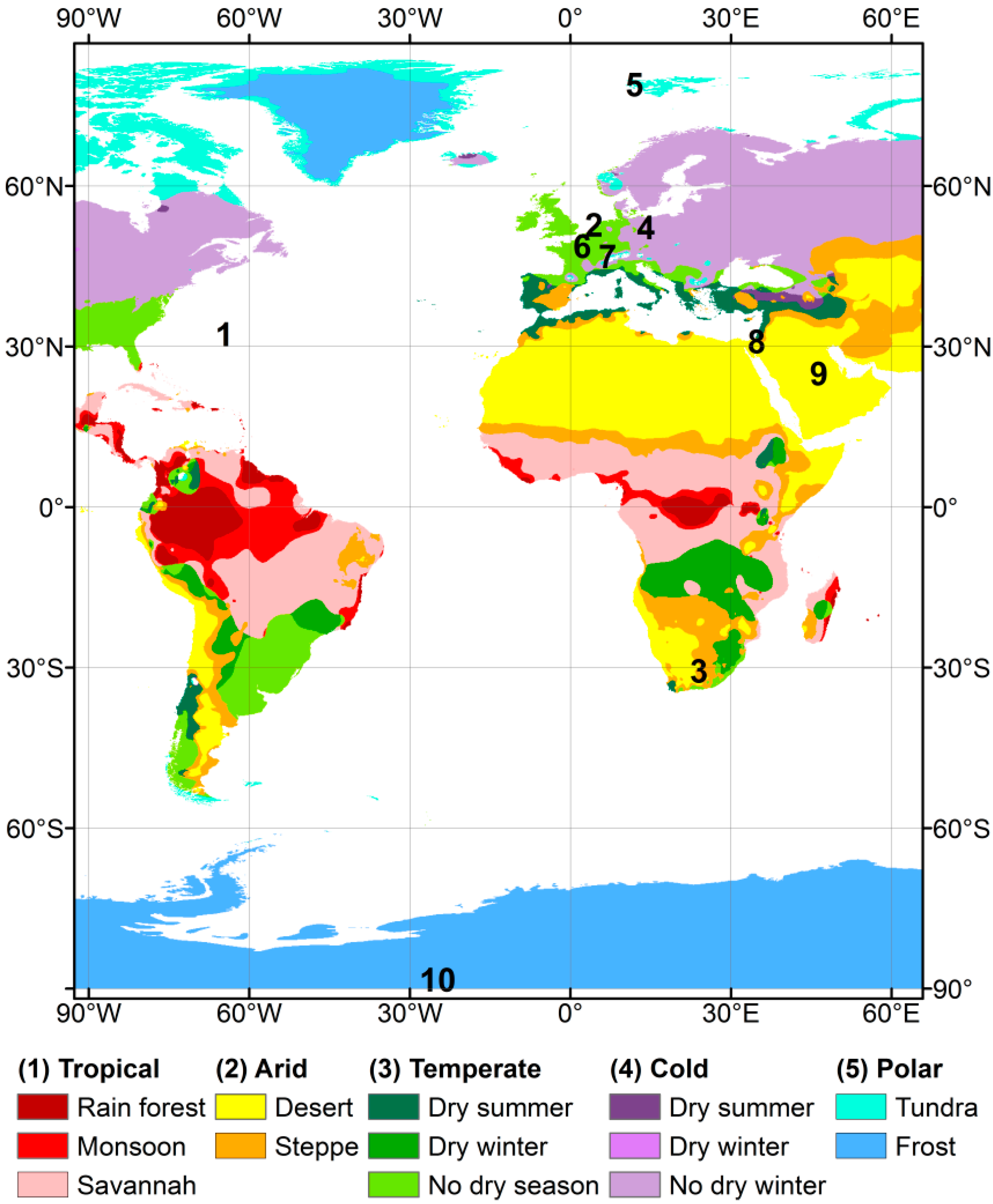
2.1. Ground-Based Cloud Cover Observations

| Site Name | Country | Lat (Deg) | Lon (Deg) | Elevation (m a.s.l.) | Mean Cloudiness (%) | Cloudiness Temporal Variability (%) | ||
|---|---|---|---|---|---|---|---|---|
| Bermuda | Bermuda | 32.27 | N | 64.68 | W | 8 | 67 | 24 |
| Cabauw | Netherlands | 51.97 | N | 4.93 | E | 0 | 68 | 20 |
| De-Aar | South-Africa | 30.66 | S | 23.99 | E | 1287 | 29 | 16 |
| Lindenberg | Germany | 52.21 | N | 14.12 | E | 125 | 70 | 17 |
| Ny-Ålesund | Norway | 78.93 | N | 11.93 | E | 11 | 74 | 13 |
| Palaiseau | France | 48.71 | N | 2.20 | E | 156 | 63 | 18 |
| Payerne | Switzerland | 46.81 | N | 6.94 | E | 491 | 66 | 17 |
| Sede-Boqer | Israel | 30.90 | N | 34.78 | E | 500 | 40 | 28 |
| Solar Village | Saudi Arabia | 24.91 | N | 46.41 | E | 650 | 23 | 14 |
| South-Pole | Antarctica | 89.98 | S | 24.79 | W | 2800 | 73 | 10 |
2.2. Satellite Overpass Times
3. Methods

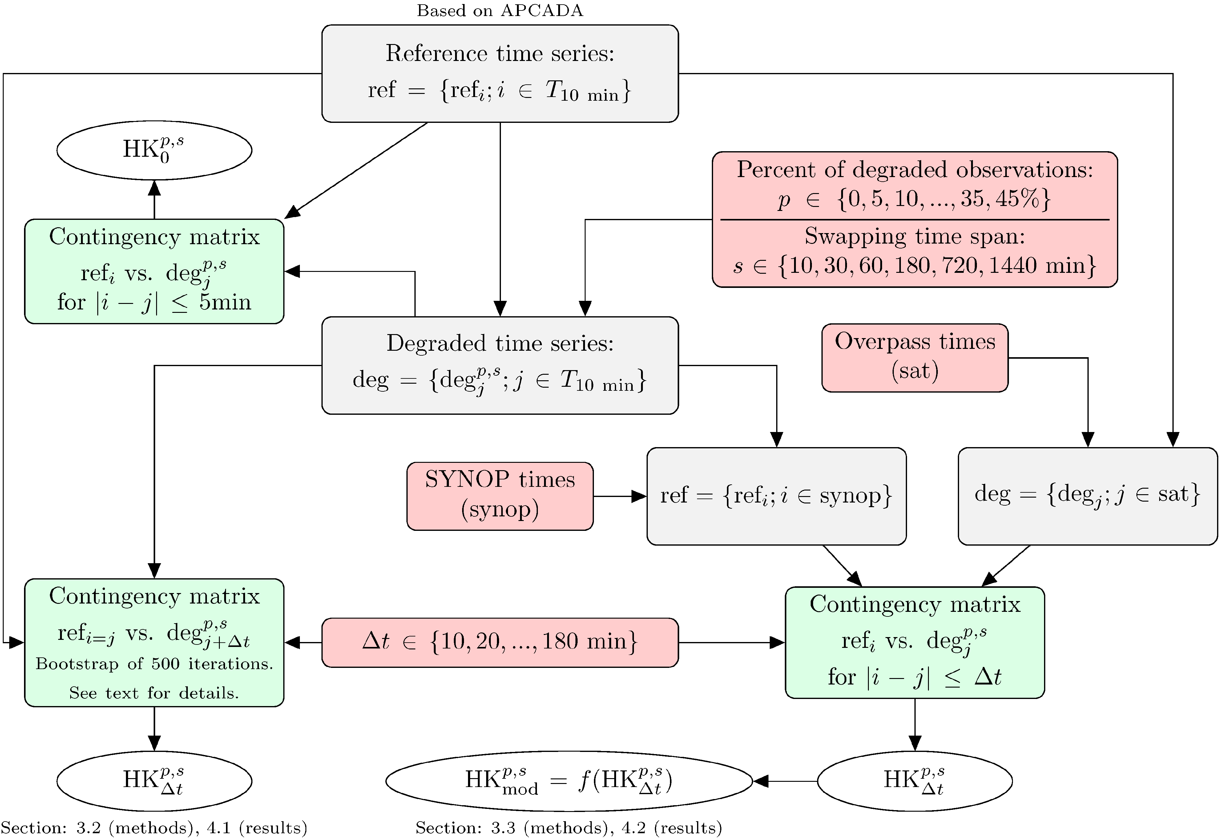
3.1. Creating a Synthetic Validation Data Set
3.2. Validation Procedure
| Ground Observation | |||
|---|---|---|---|
| Cloudy | Cloud-Free | ||
| Satellite | Cloudy | a | b |
| Cloud-free | c | d | |
3.3. Modeling the Unbiased Skill Score
4. Results
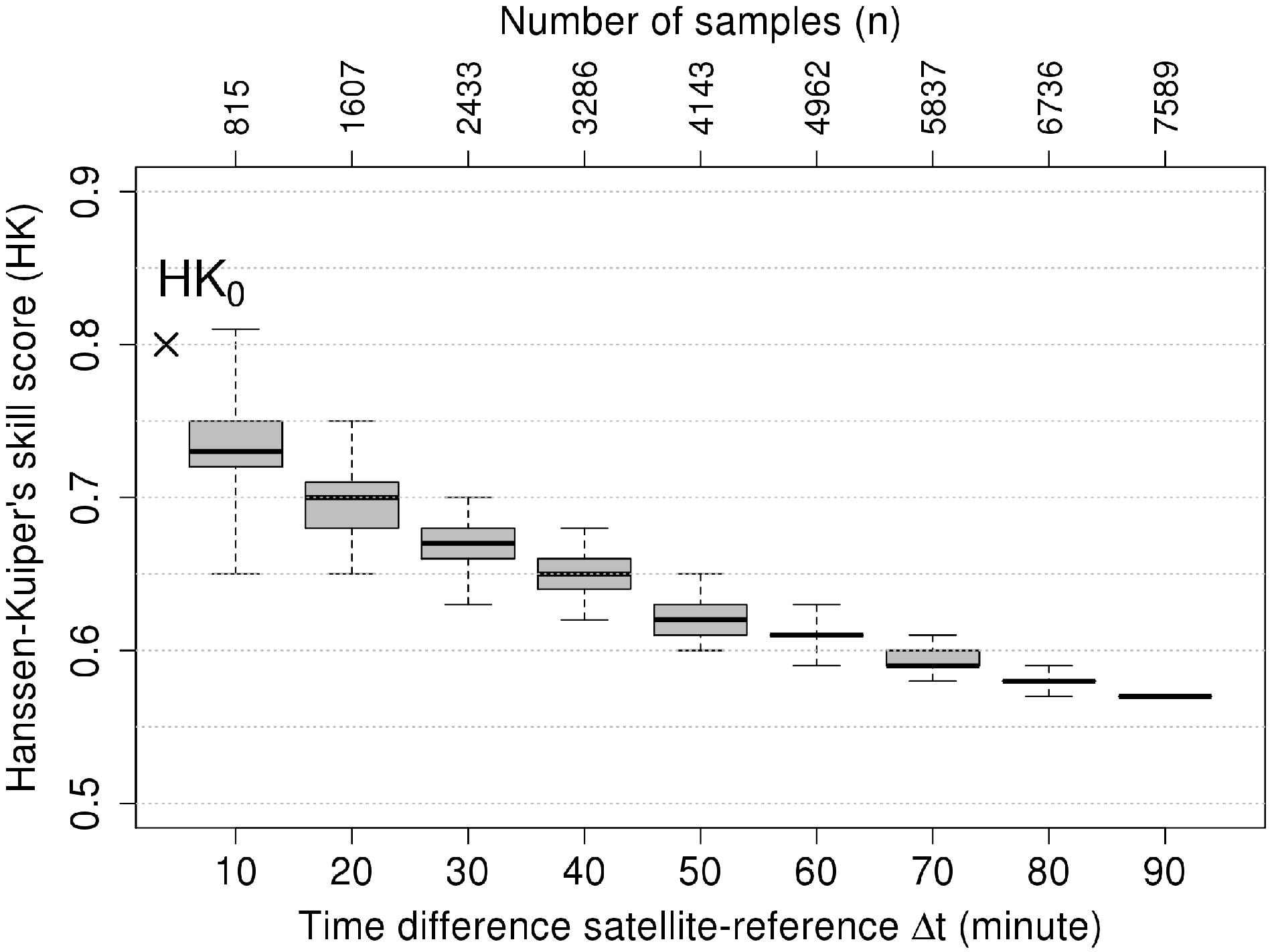
4.1. Characterizing the Skill Score Uncertainty

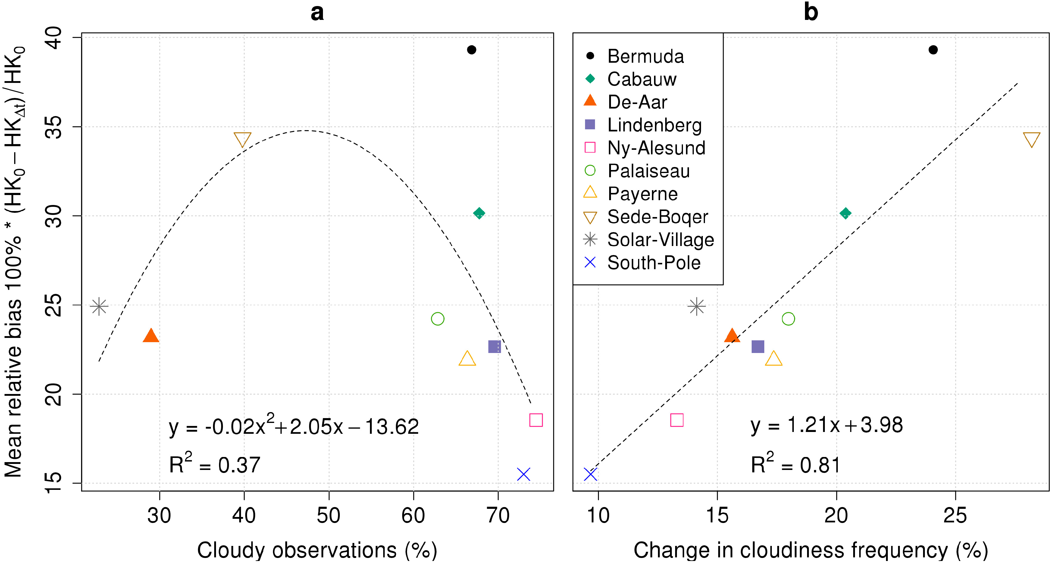
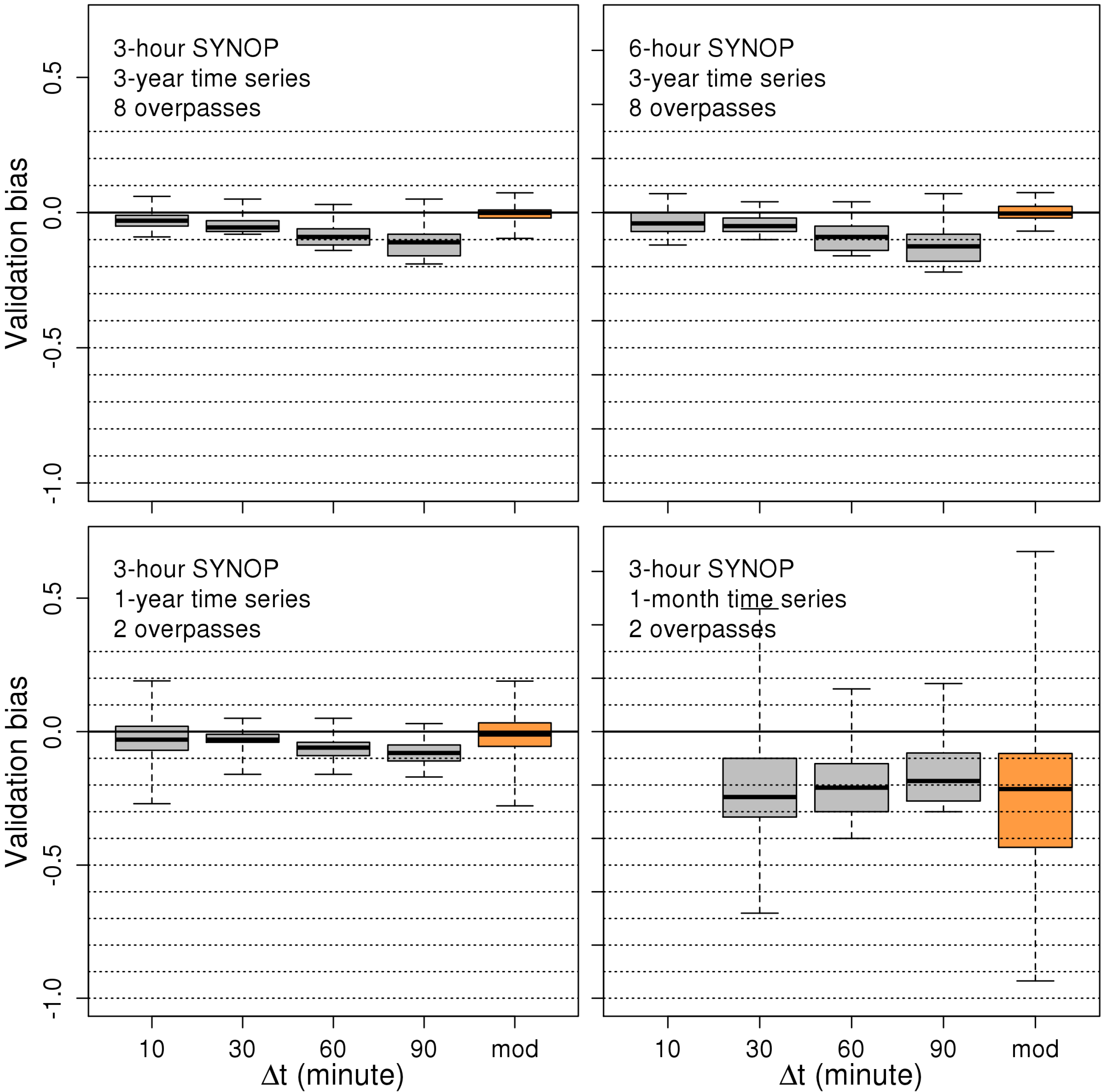
4.1.1. Bias
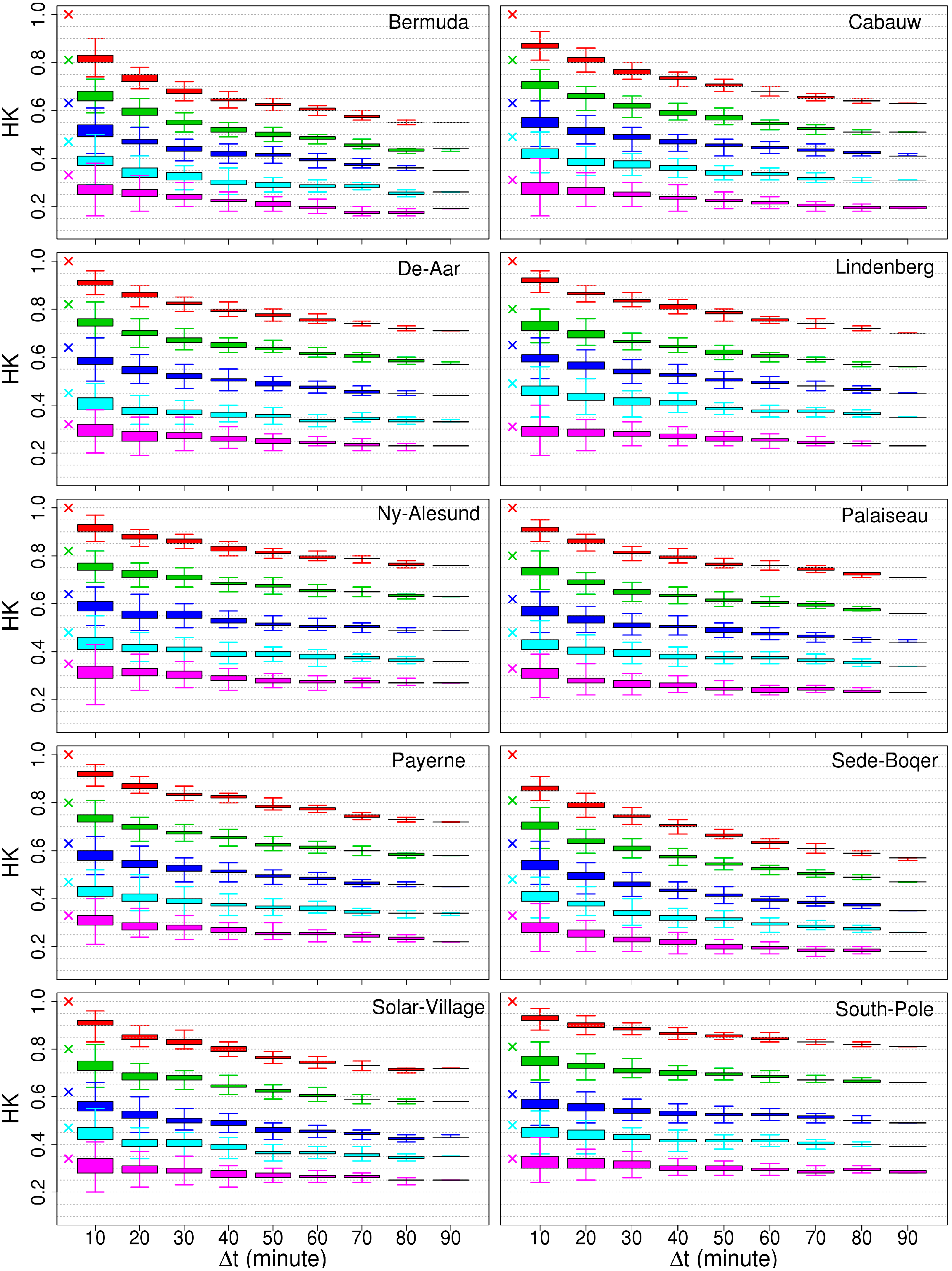


4.1.2. Spread

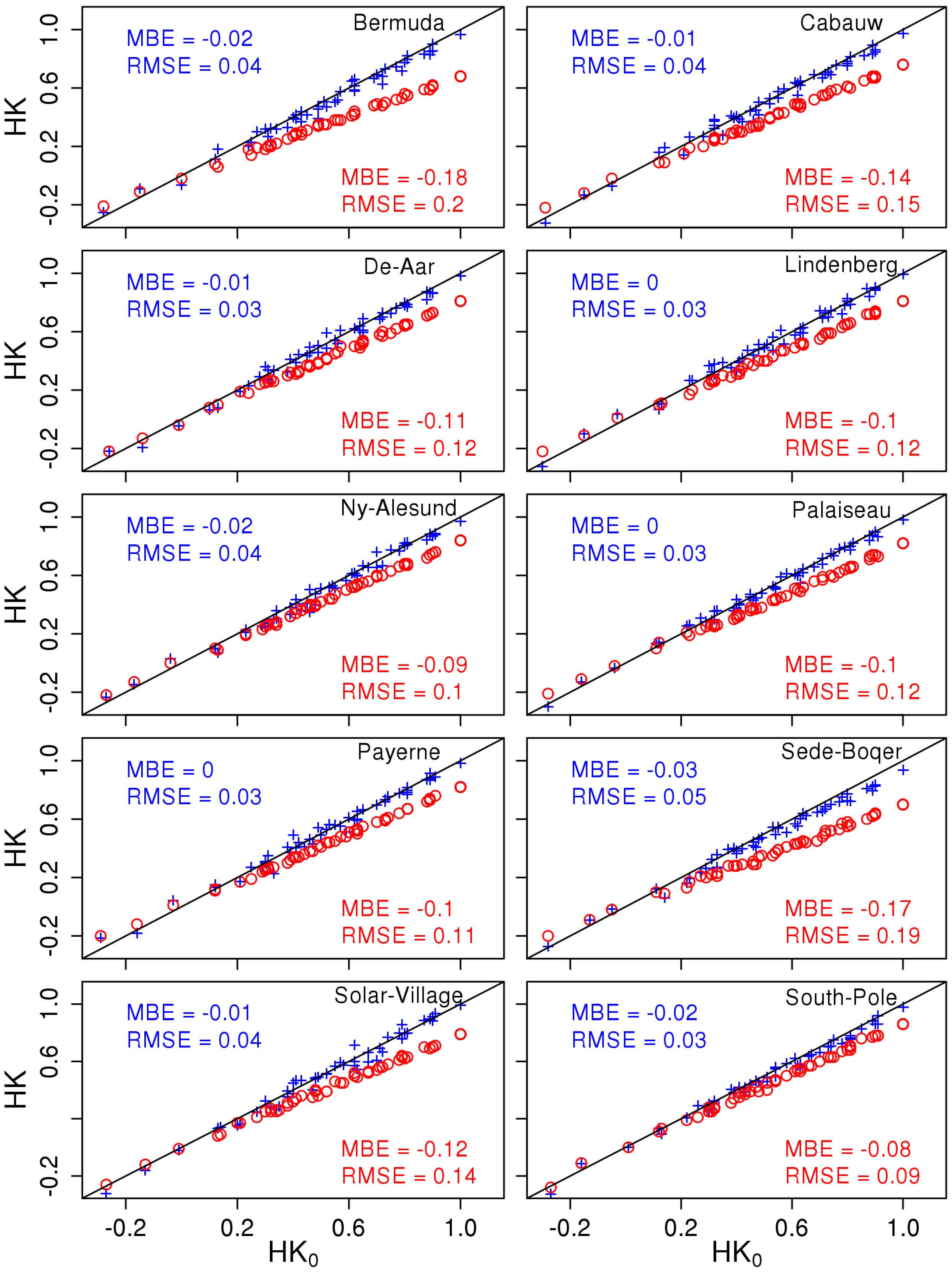
4.2. Retrieving the Unbiased Skill Score
| Time Series Length | Overpasses Per Day | SYNOP Frequency | N | HKΔt=10m | HKΔt=30m | HKΔt=60m | HKΔt=90m | HKmod | |||||
|---|---|---|---|---|---|---|---|---|---|---|---|---|---|
| n | MAE | n | MAE | n | MAE | n | MAE | n | MAE | ||||
| 3 years | 8 | 3-h | 7589 | 815 | 0.04 | 2433 | 0.07 | 4962 | 0.10 | 7589 | 0.12 | 7589 | 0.03 |
| 3 years | 8 | 6-h | 7589 | 399 | 0.05 | 1076 | 0.07 | 2050 | 0.10 | 3302 | 0.13 | 3302 | 0.04 |
| 1 year | 2 | 3-h | 646 | 69 | 0.09 | 191 | 0.08 | 410 | 0.10 | 646 | 0.12 | 646 | 0.07 |
| 1 month | 2 | 3-h | 53 | 6 | - * | 15 | 0.24 | 34 | 0.19 | 53 | 0.19 | 53 | 0.34 |

5. Discussion
5.1. Validation Inaccuracy
5.2. Modeling Unbiased Skill Score
6. Conclusions
Acknowledgments
Author Contributions
Conflicts of Interest
References
- Stephens, G.L. Cloud feedbacks in the climate system: A critical review. J. Clim. 2005, 18, 237–273. [Google Scholar] [CrossRef]
- Boucher, O.; Randall, D.; Artaxo, P.; Bretherton, C.; Feingold, G.; Forster, P.; Kerminen, V.-M.; Kondo, Y.; Liao, H.; Lohmann, U.; et al. Clouds and aerosols. In Climate Change 2013: The Physical Science Basis. Contribution of Working Group I to the Fifth Assessment Report of the Intergovernmental Panel on Climate Change; Stocker, T.F., Qin, D., Plattner, G.-K., Tignor, M., Allen, S.K., Boschung, J., Nauels, A., Xia, Y., Bex, V., Midgley, P.M., Eds.; Cambridge University Press: Cambridge, UK/New York, NY, USA, 2013; pp. 571–658. [Google Scholar]
- Global Climate Observing System (Ed.) Implementation Plan for the Global Observing System for Climate in Support of the UNFCCC; GCOS-138; Global Climate Observing System: Geneva, Switzerland, 2010.
- Global Climate Observing System (Ed.) Systematic Observation Requirements for Satellite-Based Products for Climate, 2011 Update: Supplemental Details to the Satellite-Based Component of the Implementation Plan for the Global Observing System for Climate in Support of the UNFCCC; GCOS-154; Global Climate Observing System: Geneva, Switzerland, 2011.
- Rossow, W.B.; Schiffer, R.A. Advances in understanding clouds from ISCCP. Bull. Am. Meteorol. Soc. 1999, 80, 2261–2287. [Google Scholar] [CrossRef]
- Heidinger, A.K.; Pavolonis, M.J. Gazing at cirrus clouds for 25 years through a split window. Part I: Methodology. J. Appl. Meteorol. Climatol. 2009, 48, 1100–1116. [Google Scholar] [CrossRef]
- Heidinger, A.K.; Evan, A.T.; Foster, M.J.; Walther, A. A naïve bayesian cloud-detection scheme derived from CALIPSO and applied within PATMOS-x. J. Appl. Meteorol. Climatol. 2012, 51, 1129–1144. [Google Scholar] [CrossRef]
- Schulz, J.; Albert, P.; Behr, H.-D.; Caprion, D.; Deneke, H.; Dewitte, S.; Dürr, B.; Fuchs, P.; Gratzki, A.; Hechler, P.; et al. Operational climate monitoring from space: The EUMETSAT Satellite Application Facility on Climate Monitoring (CM-SAF). Atmos. Chem. Phys. 2009, 9, 1687–1709. [Google Scholar] [CrossRef]
- Karlsson, K.-G.; Riihelä, A.; Müller, R.; Meirink, J.F.; Sedlar, J.; Stengel, M.; Lockhoff, M.; Trentmann, J.; Kaspar, F.; Hollmann, R.; et al. CLARA-A1: A cloud, albedo, and radiation dataset from 28 yr of global AVHRR data. Atmos. Chem. Phys. 2013, 13, 5351–5367. [Google Scholar] [CrossRef]
- Hollmann, R.; Merchant, C.J.; Saunders, R.; Downy, C.; Buchwitz, M.; Cazenave, A.; Chuvieco, E.; Defourny, P.; de Leeuw, G.; Forsberg, R.; et al. The ESA climate change initiative: Satellite data records for essential climate variables. Bull. Am. Meteorol. Soc. 2013, 94, 1541–1552. [Google Scholar] [CrossRef]
- Stengel, M.; Mieruch, S.; Jerg, M.; Karlsson, K.-G.; Scheirer, R.; Maddux, B.; Meirink, J.F.; Poulsen, C.; Siddans, R.; Walther, A.; et al. The clouds climate change initiative: Assessment of state-of-the-art cloud property retrieval schemes applied to AVHRR heritage measurements. Remote Sens. Environ. 2013. [Google Scholar] [CrossRef]
- Karlsson, K.-G.; Johansson, E. Multi-Sensor calibration studies of AVHRR-heritage channel radiances using the simultaneous nadir observation approach. Remote Sens. 2014, 6, 1845–1862. [Google Scholar] [CrossRef]
- Poulsen, C.A.; Watts, P.D.; Thomas, G.E.; Sayer, A.M.; Siddans, R.; Grainger, R.G.; Lawrence, B.N.; Campmany, E.; Dean, S.M.; Arnold, C. Cloud retrievals from satellite data using optimal estimation: Evaluation and application to ATSR. Atmos. Meas. Tech. Discuss. 2011, 4, 2389–2431. [Google Scholar] [CrossRef]
- Carbajal Henken, C.K.; Lindstrot, R.; Preusker, R.; Fischer, J. FAME-C: Cloud property retrieval using synergistic AATSR and MERIS observations. Atmos. Meas. Tech. Discuss. 2014, 7, 4909–4947. [Google Scholar] [CrossRef]
- Stephens, G.L.; Vane, D.G.; Boain, R.J.; Mace, G.G.; Sassen, K.; Wang, Z.; Illingworth, A.J.; O’Connor, E.J.; Rossow, W.B.; Durden, S.L.; et al. The CloudSat mission and the A-TRAIN. Bull. Am. Meteorol. Soc. 2002, 83, 1771–1790. [Google Scholar] [CrossRef]
- Winker, D.M.; Vaughan, M.A.; Omar, A.; Hu, Y.; Powell, K.A.; Liu, Z.; Hunt, W.H.; Young, S.A. Overview of the CALIPSO mission and CALIOP data processing algorithms. J. Atmos. Ocean. Technol. 2009, 26, 2310–2323. [Google Scholar] [CrossRef]
- Karlsson, K.-G.; Johansson, E. On the optimal method for evaluating cloud products from passive satellite imagery using CALIPSO-CALIOP data: Example investigating the CM SAF CLARA-A1 dataset. Atmos. Meas. Tech. 2013, 6, 1271–1286. [Google Scholar] [CrossRef]
- Dybbroe, A.; Karlsson, K.-G.; Thoss, A. NWCSAF AVHRR cloud detection and analysis using dynamic thresholds and radiative transfer modeling. Part II: Tuning and validation. J. Appl. Meteorol. 2005, 44, 55–71. [Google Scholar] [CrossRef]
- Eastman, R.; Warren, S.G. Arctic cloud changes from surface and satellite observations. J. Clim. 2010, 23, 4233–4242. [Google Scholar] [CrossRef]
- Fontana, F.; Lugrin, D.; Seiz, G.; Meier, M.; Foppa, N. Intercomparison of satellite- and ground-based cloud fraction over Switzerland (2000–2012). Atmos. Res. 2013, 128, 1–12. [Google Scholar] [CrossRef]
- Karlsson, K.-G. A 10 year cloud climatology over Scandinavia derived from NOAA advanced very high resolution radiometer imagery. Int. J. Climatol. 2003, 23, 1023–1044. [Google Scholar] [CrossRef]
- Kotarba, A.Z. A comparison of MODIS-derived cloud amount with visual surface observations. Atmos. Res. 2009, 92, 522–530. [Google Scholar] [CrossRef]
- Ma, J.; Wu, H.; Wang, C.; Zhang, X.; Li, Z.; Wang, X. Multiyear satellite and surface observations of cloud fraction over China. J. Geophys. Res. Atmos. 2014, 119, 7655–7666. [Google Scholar] [CrossRef]
- Meerkötter, R.; König, C.; Bissolli, P.; Gesell, G.; Mannstein, H. A 14-year European cloud climatology from NOAA/AVHRR data in comparison to surface observations. Geophys. Res. Lett. 2004, 31. [Google Scholar] [CrossRef]
- Henderson-Sellers, A.; Séze, G.; Drake, F.; Desbois, M. Surface-observed and satellite-retrieved cloudiness compared for the 1983 ISCCP special study area in Europe. J. Geophys. Res. Atmos. 1987, 92, 4019–4033. [Google Scholar] [CrossRef]
- Rossow, W.B.; Garder, L.C. Validation of ISCCP cloud detections. J. Clim. 1993, 6, 2370–2393. [Google Scholar] [CrossRef]
- Goodman, A.H.; Henderson-Sellers, A. Cloud detection and analysis: A review of recent progress. Atmos. Res. 1988, 21, 203–228. [Google Scholar] [CrossRef]
- Musial, J.P.; Hüsler, F.; Sütterlin, M.; Neuhaus, C.; Wunderle, S. Daytime low stratiform cloud detection on AVHRR imagery. Remote Sens. 2014, 6, 5124–5150. [Google Scholar] [CrossRef]
- Henderson-Sellers, A.; McGuffie, K. Are cloud amounts estimated from satellite sensor and conventional surface-based observations related? Int. J. Remote Sens. 1990, 11, 543–550. [Google Scholar] [CrossRef]
- Mittermaier, M. A critical assessment of surface cloud observations and their use for verifying cloud forecasts. Q. J. R. Meteorol. Soc. 2012, 138, 1794–1807. [Google Scholar] [CrossRef]
- Town, M.S.; Walden, V.P.; Warren, S.G. Cloud cover over the South Pole from visual observations, satellite retrievals, and surface-based infrared radiation measurements. J. Clim. 2007, 20, 544–559. [Google Scholar] [CrossRef]
- World Meteorological Organization (Ed.) Guide to Meteorological Instruments and Methods of Observation, 7th ed.; World Meteorological Organization: Geneva, Switzerland, 2008.
- Musial, J.P.; Hüsler, F.; Sütterlin, M.; Neuhaus, C.; Wunderle, S. Probabilistic approach to cloud and snow detection on Advanced Very High Resolution Radiometer (AVHRR) imagery. Atmos. Meas. Tech. 2014, 7, 799–822. [Google Scholar] [CrossRef]
- Ohmura, A. Baseline Surface Radiation Network (BSRN/WCRP), a new precision radiometry for climate research. Bull. Am. Meteorol. Soc. 1998, 79, 2115–2136. [Google Scholar] [CrossRef]
- Marty, C.; Philipona, R. The clear-sky index to separate clear-sky from cloudy-sky situations in climate research. Geophys. Res. Lett. 2000, 27, 2649–2652. [Google Scholar] [CrossRef]
- Dürr, B.; Philipona, R. Automatic cloud amount detection by surface longwave downward radiation measurements. J. Geophys. Res. Atmos. 2004, 109. [Google Scholar] [CrossRef]
- Ohmura, A. Physical basis for the temperature-based melt-index method. J. Appl. Meteorol. 2001, 40, 753–761. [Google Scholar] [CrossRef]
- Philipona, R.; Dürr, B.; Marty, C. Greenhouse effect and altitude gradients over the Alps—By surface longwave radiation measurements and model calculated LOR. Theor. Appl. Climatol. 2004, 77, 1–7. [Google Scholar] [CrossRef]
- Jerg, M.; Stengel, M.; Hollmann, R.; Poulsen, C. The ESA cloud CCI project: Generation of multi sensor consistent cloud properties with an optimal estimation based retrieval algorithm. In Proceedings of the 2012 EGU General Assembly Conference Abstracts, Vienna, Austria, 22–27 April 2012.
- Stapelberg, S.; Jerg, M.; Stengel, M.; Hollmann, R.; Lindstrot, R.; Poulsen, C. ESA Cloud CCI: Generation of optimal estimation based, multi-sensor cloud property data set from AVHRR heritage measurements. In Proceedings of the 2013 EGU General Assembly Conference Abstracts, Vienna, Austria, 7–12 April 2013.
- Foster, M.J.; Heidinger, A. PATMOS-x: Results from a diurnally corrected 30-yr satellite cloud climatology. J. Clim. 2013, 26, 414–425. [Google Scholar] [CrossRef]
- Wilks, D.S. Statistical Methods in the Atmospheric Sciences, 2nd ed.; Elsevier: Amsterdam, The Netherlands, 2006. [Google Scholar]
- Efron, B. Bootstrap methods: Another look at the Jackknife. Ann. Stat. 1979, 7, 1–26. [Google Scholar] [CrossRef]
© 2014 by the authors; licensee MDPI, Basel, Switzerland. This article is an open access article distributed under the terms and conditions of the Creative Commons Attribution license (http://creativecommons.org/licenses/by/4.0/).
Share and Cite
Bojanowski, J.S.; Stöckli, R.; Tetzlaff, A.; Kunz, H. The Impact of Time Difference between Satellite Overpass and Ground Observation on Cloud Cover Performance Statistics. Remote Sens. 2014, 6, 12866-12884. https://doi.org/10.3390/rs61212866
Bojanowski JS, Stöckli R, Tetzlaff A, Kunz H. The Impact of Time Difference between Satellite Overpass and Ground Observation on Cloud Cover Performance Statistics. Remote Sensing. 2014; 6(12):12866-12884. https://doi.org/10.3390/rs61212866
Chicago/Turabian StyleBojanowski, Jędrzej S., Reto Stöckli, Anke Tetzlaff, and Heike Kunz. 2014. "The Impact of Time Difference between Satellite Overpass and Ground Observation on Cloud Cover Performance Statistics" Remote Sensing 6, no. 12: 12866-12884. https://doi.org/10.3390/rs61212866
APA StyleBojanowski, J. S., Stöckli, R., Tetzlaff, A., & Kunz, H. (2014). The Impact of Time Difference between Satellite Overpass and Ground Observation on Cloud Cover Performance Statistics. Remote Sensing, 6(12), 12866-12884. https://doi.org/10.3390/rs61212866