Satellite Observations of Wind Farm Impacts on Nocturnal Land Surface Temperature in Iowa

Abstract

Wind farms (WFs) are believed to have an impact on lower boundary layer meteorology. A recent study examined satellite-measured land surface temperature data (LST) and found a local nighttime warming effect attributable to a group of four large WFs in Texas. This study furthers their work by investigating the impacts of five individual WFs in Iowa, where the land surface properties and climate conditions are different from those in Texas. Two methods are used to assess WF impacts: first, compare the spatial coupling between the LST changes (after turbine construction versus before) and the geographic layouts of the WFs; second, quantify the LST difference between the WFs and their immediate surroundings (non-WF areas). Each WF shows an irrefutable nighttime warming signal relative to the surrounding areas after their turbines were installed, and these warming signals are generally coupled with the geographic layouts of the wind turbines, especially in summer. This study provides further observational evidence that WFs can cause surface warming at nighttime, and that such a signal can be detected by satellite-based sensors.

1. Introduction

Wind turbines extract kinetic energy from the atmospheric flow to generate electricity. Consequently, the spinning blades enhance vertical mixing and increase turbulence within a few hundred meters above the ground [1]. In a wind farm (WF), the collective effects of multiple turbines can theoretically alter near-surface atmospheric boundary layer (ABL) fluxes of heat, momentum and moisture, leading to noticeable changes in local meteorology.

Recent modeling studies [2,3,4,5] have simulated local WF impacts by approximating wind turbines as massless, elevated sinks of kinetic energy and sources of turbulent kinetic energy. Relative warming of the air below the turbine rotor area at nighttime has been noted, caused by a vertical redistribution of the air due to turbine-enhanced vertical mixing and turbulence. In a typical nighttime ABL with strong stable stratification (i.e., $\text{∂θ}/\text{∂z}$ >> 0) and laminar low-level flow [6,7], enhanced vertical mixing would act to bring warm air downward and cool air upward, thus allowing more heat to be transferred from the air to the radiatvely-cooled ground [3]. Similar vertical redistribution of heat has been found with a large-eddy simulation of a WF [8]. Impacts of WFs also apply to surface sensible and latent heat fluxes, depending on the static stability and total water mixing ratio lapse rate of the atmosphere. Nighttime surface sensible heat flux is typically negative, with heat transport from the atmosphere to the ground, and so WFs bringing warmer air to the surface makes the surface sensible heat flux more negative [3].

Few studies so far have documented observational evidence of WF impacts on local meteorology. Baidya Roy and Traiteur [9] observed a slight late-night warming effect of about 1 °C for a small WF in California by comparing 5-m air temperature measurements from two meteorological towers, upwind and downwind of the WF, for a 53-day summertime period. Smith et al. [10] observed a nighttime warming effect of 1.9 °C for a large WF in the Midwest U.S. by comparing 2-m air temperatures from a WF-waked area to a non-waked area, for a 47-day springtime period. Rajewski et al. [11] observed several individual periods with a significant warming of 1.0–1.5 °C within a group of 13 turbines in a WF in Iowa, using 9-m tower data from a 42-day summertime period. The results from these studies are significant but only indicate WF impacts from point measurements over short time periods.

Surface measurements near or within WFs are not easy to obtain if the data or WFs are privately owned, and the spatial and temporal coverage of publicly available data may not be sufficient for long-term studies of WF impacts on larger scales. Alternatively, satellite-based remote sensing instruments can consistently provide observations over broad areas for long periods of time. For instance, Zhou et al. [12] studied nine years of summertime and wintertime land surface temperature data (LST) from the Moderate Resolution Imaging Spectroradiometer (MODIS) instruments onboard NASA’s Terra and Aqua satellites. They chose an area centered on a large group of four WFs in Texas that were built in phases, and they observed a nighttime warming rate of 0.72 °C per decade over the WFs in the summer, relative to nearby non-WF areas. No significant daytime impacts were found. They ruled out changes in vegetation greenness, land cover and surface albedo as the possible causes for the warming signal. Zhou et al. [13] examined seasonal and diurnal variations of such impacts for the same WFs in Texas. Their results consistently showed a nighttime WF warming of 0.31–0.70 °C across all seasons for both the Terra and Aqua measurements, with the largest warming effect occurring at ~10:30 p.m. in the summer. Their results for the daytime were noisy and insignificant. Zhou et al. [14] also ruled out the possibility that the warming signal could be an artifact of varied surface topography in and around the WFs.

The MODIS dataset and methodology used in Zhou et al. [13] are applied here, but for five individual WFs in Iowa. The Texas WFs examined previously [12,13,14] are built on semi-arid grasslands and complex terrain, whereas the WFs examined here are built mostly on farmlands and relatively smoother topography. Areas with different land surface properties can have disparate fluxes of sensible and latent heat. For a field study, Doran et al. [15] found the measured surface sensible heat flux over semi-arid grasslands to be higher than that over adjacent irrigated farmlands by a factor of four or more, and the latent heat flux differences were nearly opposite. The effects of these sensible and latent heat flux differences eventually propagate through the ABL. Because the WFs in Texas and Iowa are built on such differing land surface types, and therefore have drastically different ABL and climate characteristics, the primary question of this study is whether the WFs in Iowa would yield results similar to previous studies. This paper furthers the work of Zhou et al. [13] and demonstrates that their results are not unique to the Texas WFs on semi-arid grassland.

2. Data and Methodology

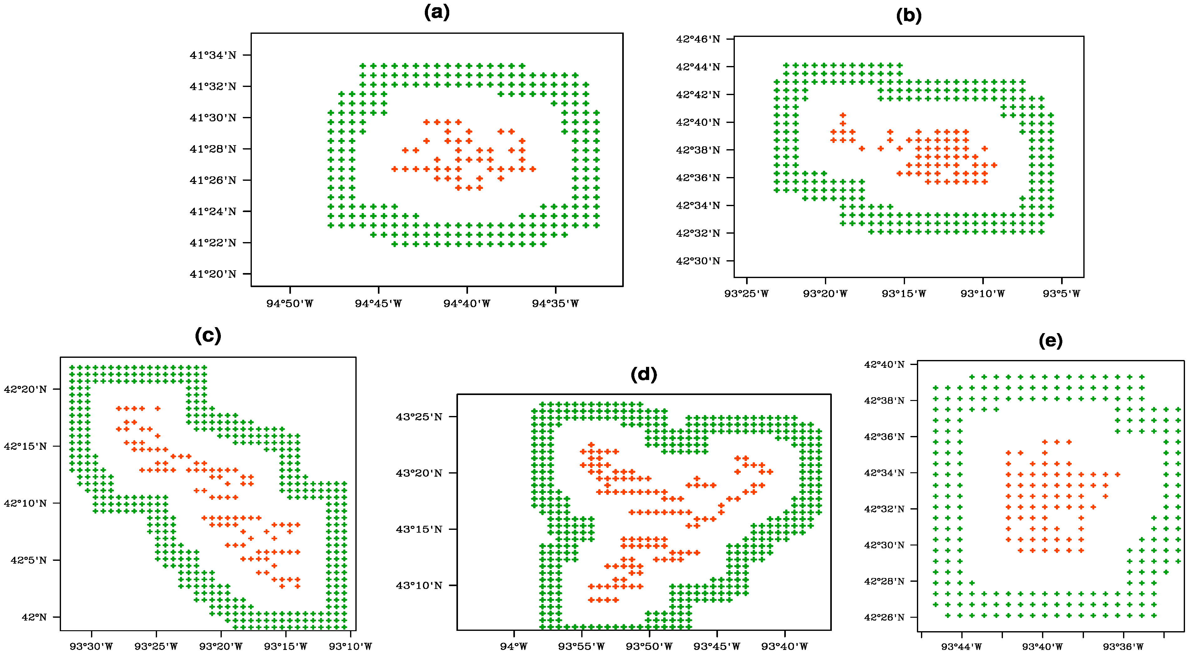
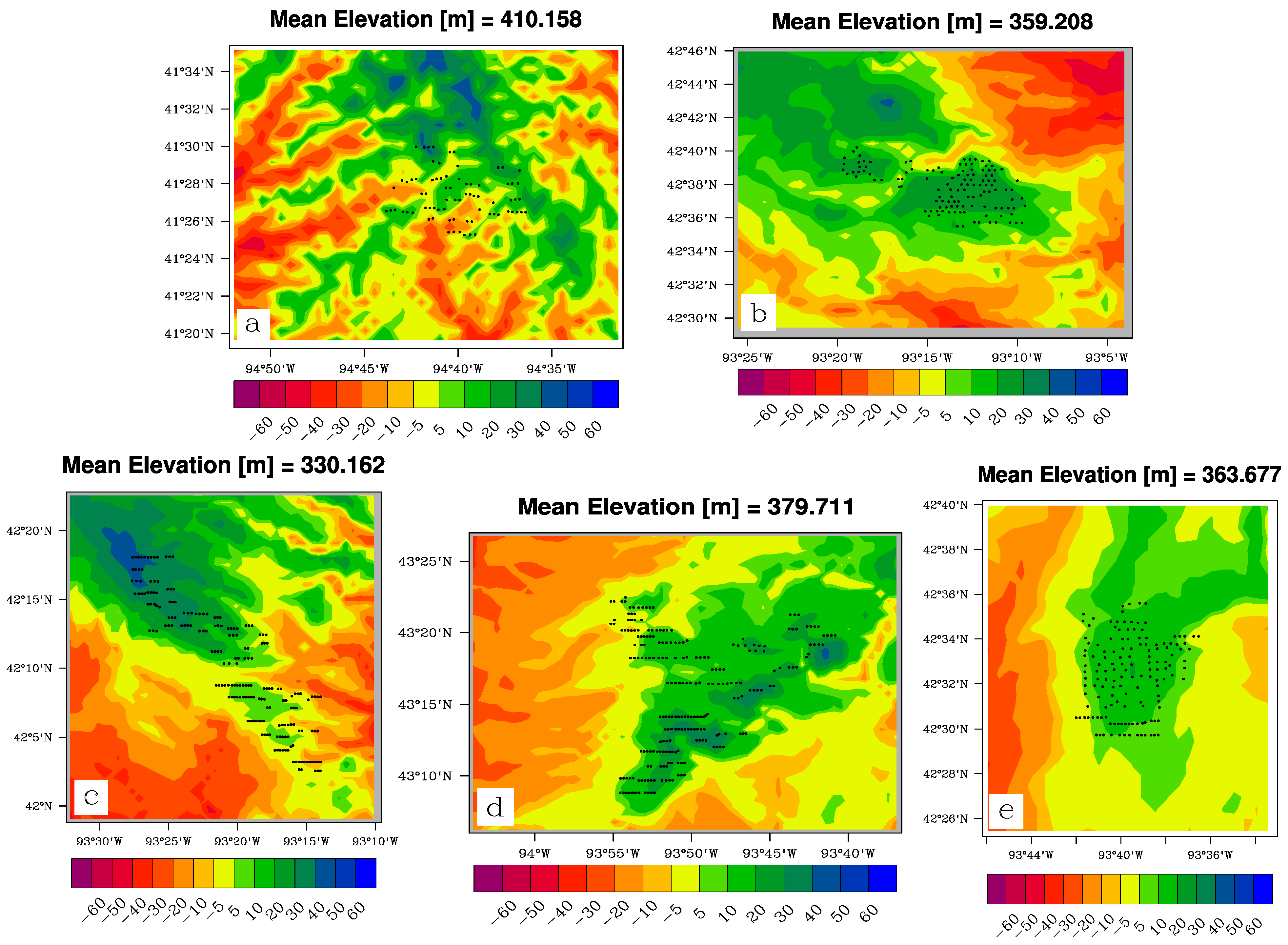
The five WFs in this study are consistently labeled a through e in all figures and tables. Table 1 gives the construction dates and number of turbines for each WF. This information is publicly available from various sources [16]. Figure 1 shows elevation plots for each WF region using GTOPO30 data from the U.S. Geological Survey [17]. The terrain over each WF region is relatively flat, with the elevation ranges not exceeding 120 m. The majority of each WF region consists of agricultural land. The precise locations of turbines in each WF were determined using latitude/longitude coordinates from the Federal Aviation Administration’s Obstruction Evaluation/Airport Airspace Analysis database (FAA OE/AAA) [18]. Obstructions over a certain height must be reported, and the FAA logs the construction dates and types of obstructions. The existence of each individual turbine was verified for this study using Google Earth, and coordinates for nonexistent turbines were removed from the list.

Table 1. Construction dates and number of turbines for each wind farm (WF).

WF	a	b	c	d	e
Year	2008	2009	2008–2009	2008–2009	2005
Number	76	121	200	224	135

Table 1. Construction dates and number of turbines for each wind farm (WF).

WF	a	b	c	d	e
Year	2008	2009	2008–2009	2008–2009	2005
Number	76	121	200	224	135

Eleven full years of MODIS 8-day LST data (MOD11A2 and MYD11A2) [19] are used here, beginning with 2003 when both the Terra and Aqua satellites had complete years of data, through 2013. Each satellite takes two measurements per day for a given location: Terra at ~10:30 a.m. and ~10:30 p.m., and Aqua at ~1:30 p.m. and ~1:30 a.m., local solar time. Thus, there are two nighttime measurements and two daytime measurements per day. LST is the radiometric temperature derived from surface emission and is closely related to land surface radiative properties [20]. The 8-day LST products are 2–8 day averages of daily products, depending on the gaps in the data, and they represent the best quality data retrieval possible from clear-sky conditions [21]. The resolution of the MODIS data is approximately 1 km on a sinusoidal projection, and the data are re-projected onto a 0.01° resolution grid of pixels that are roughly 1.1 km². The LST data are produced with various quality flags based on cloud interference and measurement errors, but no LST data are produced for pixels that are covered by clouds. This study uses all available LST data (i.e., all data not flagged with bad quality), allowing the highest number of pixels to be used. Additionally, data with different quality controls are examined. The higher quality assurance criteria include fewer composites in the 8-day LST averages.

Figure 1. Topography for each WF (a–e) in terms of the deviation from the mean elevation (m) over the region. Black dots represent individual turbines.

Figure 1. Topography for each WF (a–e) in terms of the deviation from the mean elevation (m) over the region. Black dots represent individual turbines.

Pixel-level anomalies were produced for each season, year and MODIS measurement time. First, monthly means were calculated using the 8-day LST data. Monthly climatology values were calculated from the monthly means. Then, monthly anomalies were calculated by subtracting the monthly climatology from each pixel. Seasonal means and anomalies were created by combining monthly values, i.e., winter is Dec-Jan-Feb (DJF), spring is Mar-Apr-May (MAM), summer is Jun-Jul-Aug (JJA), fall is Sep-Oct-Nov (SON), and an annual average (ANN) for all months.

Two methods are used to assess WF impacts on LST at pixel- and region-aggregated levels for each season. The first method calculates the pixel-level LST differences between the later years’ mean anomaly values (after WF construction) and the earlier years’ mean anomaly values (before WF construction). For example, for a WF built in 2008, it is the anomaly difference between (2009–2013) and (2003–2007). By plotting pixel-level LST anomalies, spatial patterns in the LST changes can be compared to the geographic layouts of the WFs. Each WF has a unique geographic layout of turbines, therefore any WF impacts should resemble the WF layout to some extent. The second method calculates the difference between the mean anomaly value over wind farm pixels (WFPs) and the mean anomaly value over nearby non-WF pixels (NNWFPs), for each year. Pixels with one or more turbines present are defined as WFPs, and NNWFPs are selected in an area around the WFPs that is 3–4 pixels wide and 3–4 pixels away from the nearest WFPs, so the immediate surroundings are represented without being impacted by the WFs. This leaves about 3–4 km between the WFPs and NNWFPs, which is enough distance for the WF wake to no longer be detectable [10]. Figure 2 shows plots of WFPs and NNWFPs for each WF region. Both methods are beneficial because they use data over a large spatial domain for a long period of time. However, throughout the long period of the data there are undoubtedly days when the WFs may not have been fully operational, whether for weather or maintenance reasons, but there is no way to filter non-operational days from the 8-day LST product. Assuming it is unusual for a WF to be non-operational, those days should not have a significant impact on a long-term averages.

Figure 2. Wind farm pixels (WFPs) in orange, containing at least one turbine, and nearby non-wind-farm pixels (NNWFPs) in green, for each WF (a–e). The pixel resolution is 0.01°, or roughly 1.1 km².

Figure 2. Wind farm pixels (WFPs) in orange, containing at least one turbine, and nearby non-wind-farm pixels (NNWFPs) in green, for each WF (a–e). The pixel resolution is 0.01°, or roughly 1.1 km².

3. Results and Discussion

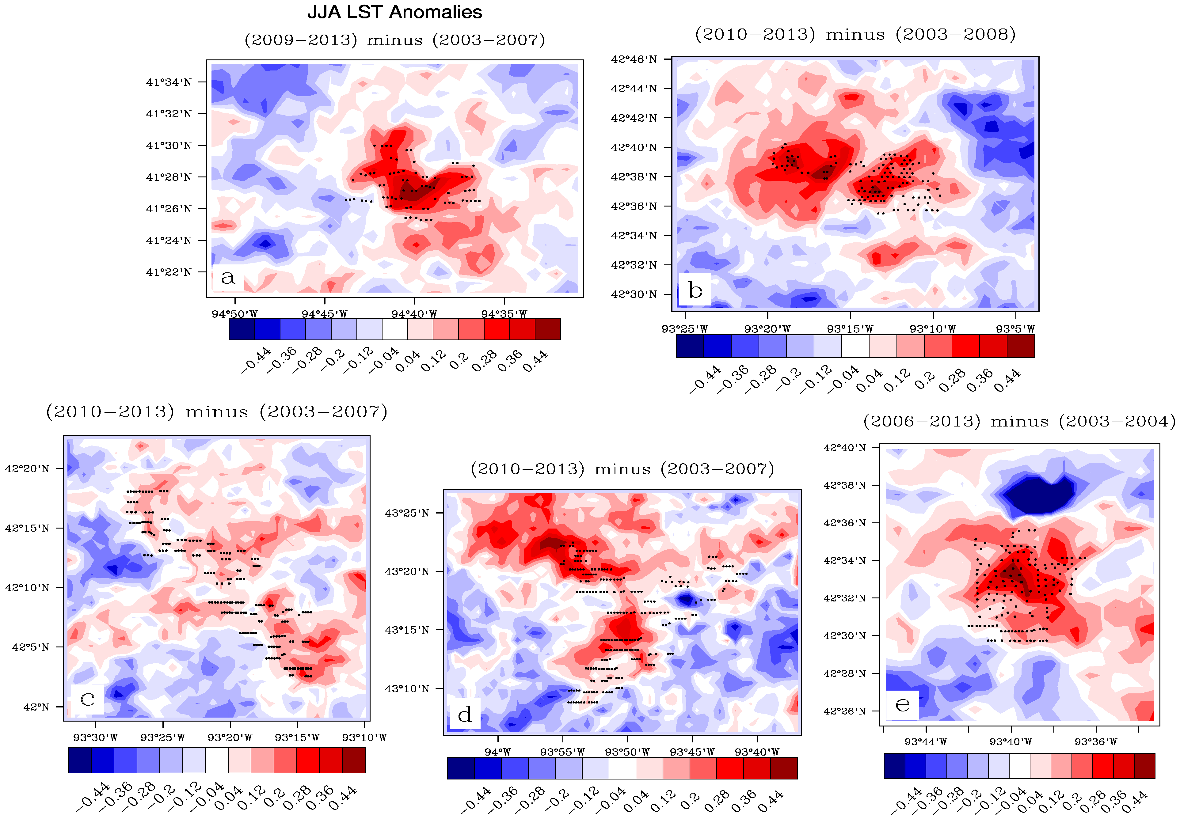
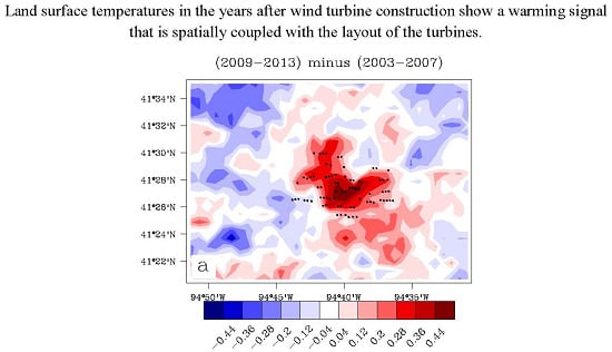
Figure 3 shows the pixel-level LST anomaly differences, post- minus pre-turbine-construction years, for each WF for JJA at ~10:30 p.m. Note that a regional mean value is removed from the LST anomaly difference to highlight the pixel-level LST changes relative to the regional mean [13]. Thus, the red contours indicate areas where the LST anomaly difference between later years and earlier years is greater than the region-average LST change, while the blue contours are areas with LST anomaly differences below that average. There is a relative warming effect for each WF, indicated by positive anomalies of 0.12–0.44 °C, that is spatially collocated with the turbines. This spatial coupling suggests that the WFs are likely causing the warming effect, which is consistent with previous studies. 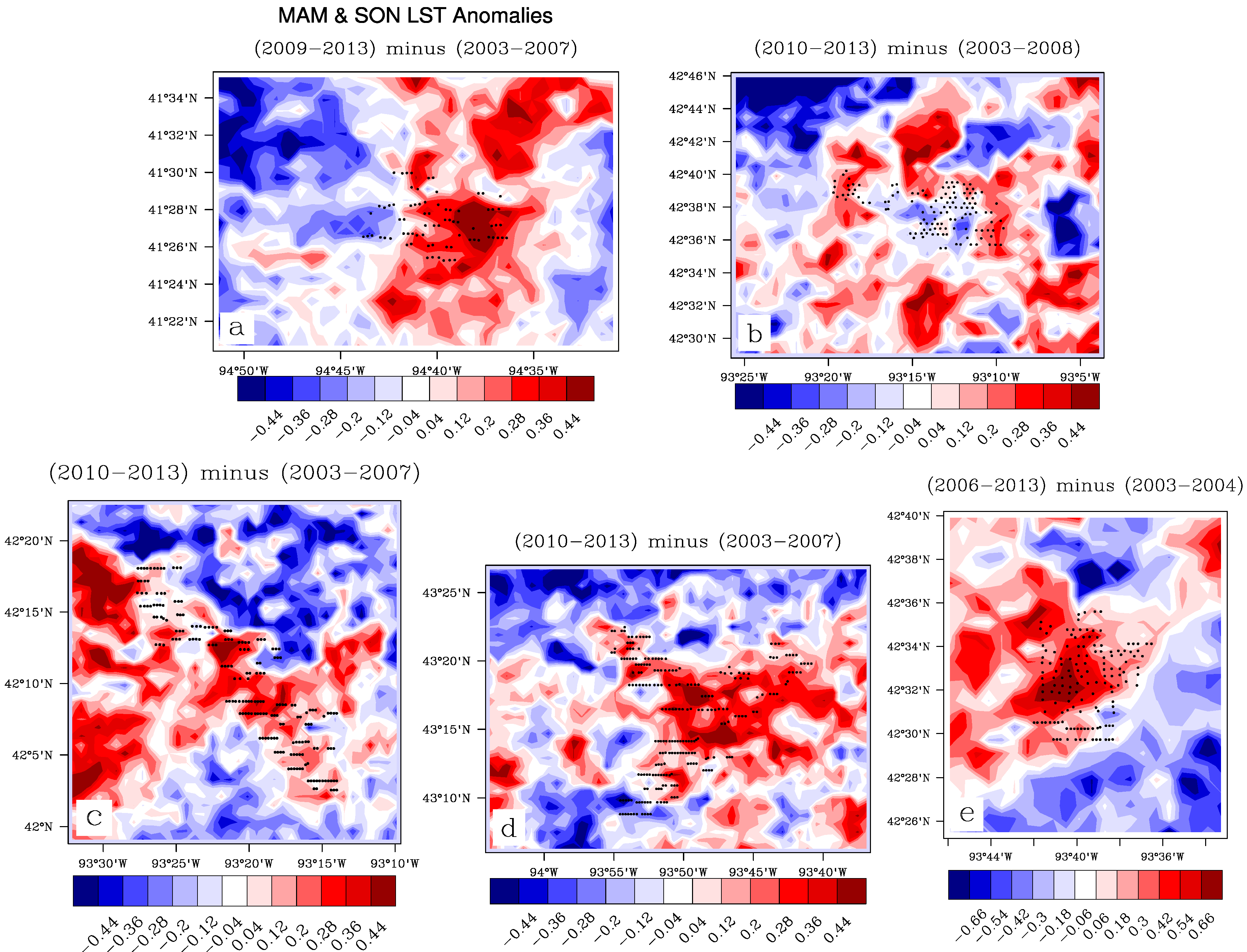Figure 4 shows the same pixel-level anomaly differences as Figure 3, but for an average of MAM and SON. The DJF plots are very noisy compared to the other seasons, with practically no LST anomaly signals that are spatially coupled with the WF layouts, and are therefore not included. Significant high-frequency LST variability due to extreme weather events such as cold fronts and the associated changes in land surface properties (e.g., snow cover) likely mask any small low-frequency WF-induced warming signals in DJF. Figure 4 demonstrates that the nighttime WF-warming effect does not occur only in the summer, but compared with Figure 3 it is evident that JJA is the best season for noticing warming effects that are spatially coupling with the layouts of the WFs.

Figure 3. Pixel-level anomaly differences, post- minus pre-turbine-construction years, for each WF (a–e), for Jun-Jul-Aug (JJA) at ~10:30 p.m. Black dots represent individual turbines. Note that a regional mean value is removed from the land surface temperature (LST) anomaly difference to highlight pixel-level LST changes relative to the regional mean [13].

Figure 3. Pixel-level anomaly differences, post- minus pre-turbine-construction years, for each WF (a–e), for Jun-Jul-Aug (JJA) at ~10:30 p.m. Black dots represent individual turbines. Note that a regional mean value is removed from the land surface temperature (LST) anomaly difference to highlight pixel-level LST changes relative to the regional mean [13].

In both Figure 3 and Figure 4, there is a small area of strong negative anomalies in excess of −0.44 °C just north of WF e. This feature was investigated further, and it is attributed to a small lake with relatively warmer anomalies in earlier years, thus making the anomaly difference negative. The change in the lake’s signal could be due to a change in water surface area, but further speculation is beyond the scope of this study. There are other non-WF areas in each region with warming and cooling anomalies associated with either natural LST variability and/or errors due cloud and aerosol contamination [13]. A low-pass filtering technique such as empirical orthogonal function (EOF) analysis can reduce high-frequency LST variations and leave some persistent WF-warming signals [14]. Nevertheless, the spatial and temporal averaging used here should remove most high-frequency signals in the data, and the remaining residuals cannot coincidentally create the strong spatial coupling between the warming signals and the turbines [13].

Figure 4. Pixel-level anomaly differences, post- minus pre-turbine-construction years, for each WF (a–e), for Mar-Apr-May (MAM) and Sep-Oct-Nov (SON) at ~10:30 p.m. Black dots represent individual turbines. Note that a regional mean value is removed from the land surface temperature (LST) anomaly difference to highlight pixel-level LST changes relative to the regional mean [13].

Figure 4. Pixel-level anomaly differences, post- minus pre-turbine-construction years, for each WF (a–e), for Mar-Apr-May (MAM) and Sep-Oct-Nov (SON) at ~10:30 p.m. Black dots represent individual turbines. Note that a regional mean value is removed from the land surface temperature (LST) anomaly difference to highlight pixel-level LST changes relative to the regional mean [13].

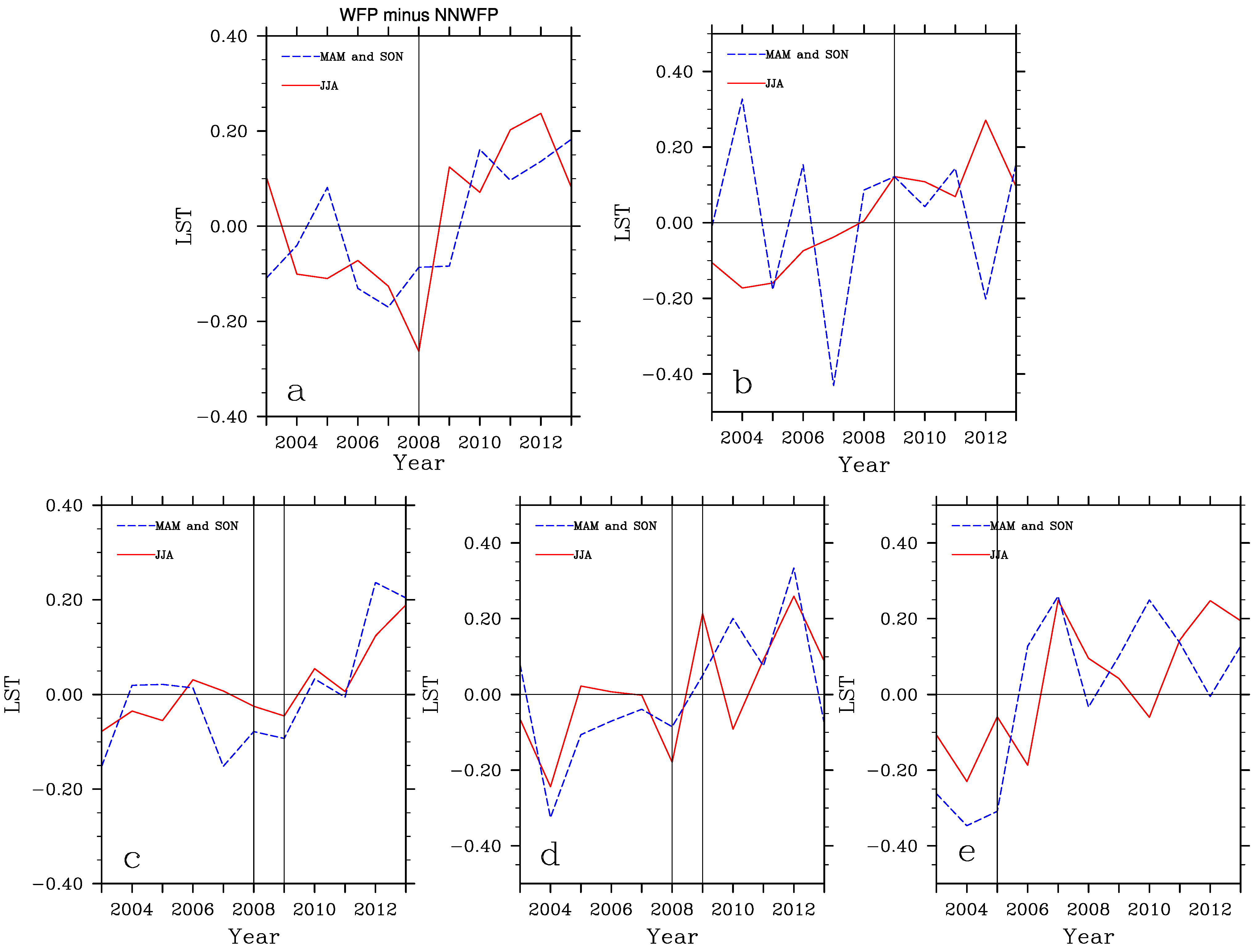
Figure 5 shows the interannual variability of the difference between WFP and NNWFP LST anomalies, for each WF at ~10:30 p.m. in JJA, as well as MAM and SON. Positive values indicate that WFP anomalies are greater than NNWFP anomalies. Vertical reference lines indicate turbine construction years. The positive shift (0–0.20 °C) in the WFP-NNWFP LST anomaly differences after turbine construction, relative to the negative values (−0.20–0) before turbine construction, indicates that WFPs undergo a relative warming rate compared to the NNWFPs, which is consistent with the findings of Zhou et al. [13]. These areal mean warming values are slightly smaller in magnitude compared to the maximum warming signals in the pixel-level anomaly differences because stronger warming anomalies tend to occur in the middle of the WFs, where the collective wake effects are larger, whereas the warming anomalies tend to be weaker closer to the edges of the WFs.

Table 2 shows mean WFP-NNWFP LST differences (in degrees Celsius) from before to after turbine construction, for MAM, JJA and SON at ~10:30 p.m. Positive values represent a mean warming effect over the WFPs relative to NNWFPs in later years compared to earlier years. Nearly all the seasons for each WF show positive values. For reasons discussed previously, Table 2 excludes values for DJF, and therefore ANN as well. The WFP-NNWFP LST difference values in DJF are not as meaningful as the values for the other seasons which had good spatial coupling between the warming signals and the WFs. The WFPs and NNWFPs are chosen in a way such that spatial patterns in LST changes could be quantified. Without a spatially coupled signal, positive and negative values do not indicate any sort of WF-warming or cooling effects, only that the detected LST variability over the chosen pixels yielded such a number. With that in mind, the negative value in Table 2 for WF b in MAM does not necessarily mean there is a WF-cooling effect, but rather that in the absence of any discernible WF signal the natural LST variability over WFPs and NNWFPs might happen to yield a negative value. Seasonal variations of the ABL likely contribute to these varying signals or lack thereof.

Figure 5. Interannual variability of the WFP-NNWFP mean LST anomaly difference at ~10:30 p.m. for JJA (solid) and MAM and SON (dashed), for each WF (a–e). The vertical reference lines mark the years when the WFs were under construction.

Figure 5. Interannual variability of the WFP-NNWFP mean LST anomaly difference at ~10:30 p.m. for JJA (solid) and MAM and SON (dashed), for each WF (a–e). The vertical reference lines mark the years when the WFs were under construction.

Table 2. Mean WFP-NNWFP LST anomaly differences for each WF at ~10:30 p.m. Values are calculated as the difference between mean WFP-NNWFP differences after and before turbine construction.

WF	a	b	c	d	e
MAM	0.037	−0.093	0.152	0.213	0.365
JJA	0.184	0.227	0.119	0.143	0.259
SON	0.202	0.181	0.181	0.238	0.485

Table 2. Mean WFP-NNWFP LST anomaly differences for each WF at ~10:30 p.m. Values are calculated as the difference between mean WFP-NNWFP differences after and before turbine construction.

WF	a	b	c	d	e
MAM	0.037	−0.093	0.152	0.213	0.365
JJA	0.184	0.227	0.119	0.143	0.259
SON	0.202	0.181	0.181	0.238	0.485

The results thus far have used all data without any quality flags. LST anomalies over each WF were also examined using different quality assurance (QA) controls. Altering the QA criteria can improve the overall LST data quality, but the number of LST retrievals used for spatial and temporal averaging is reduced, consequently resulting in uncertainties in LST variations due to the sampling heterogeneity over different periods and different pixels [13]. 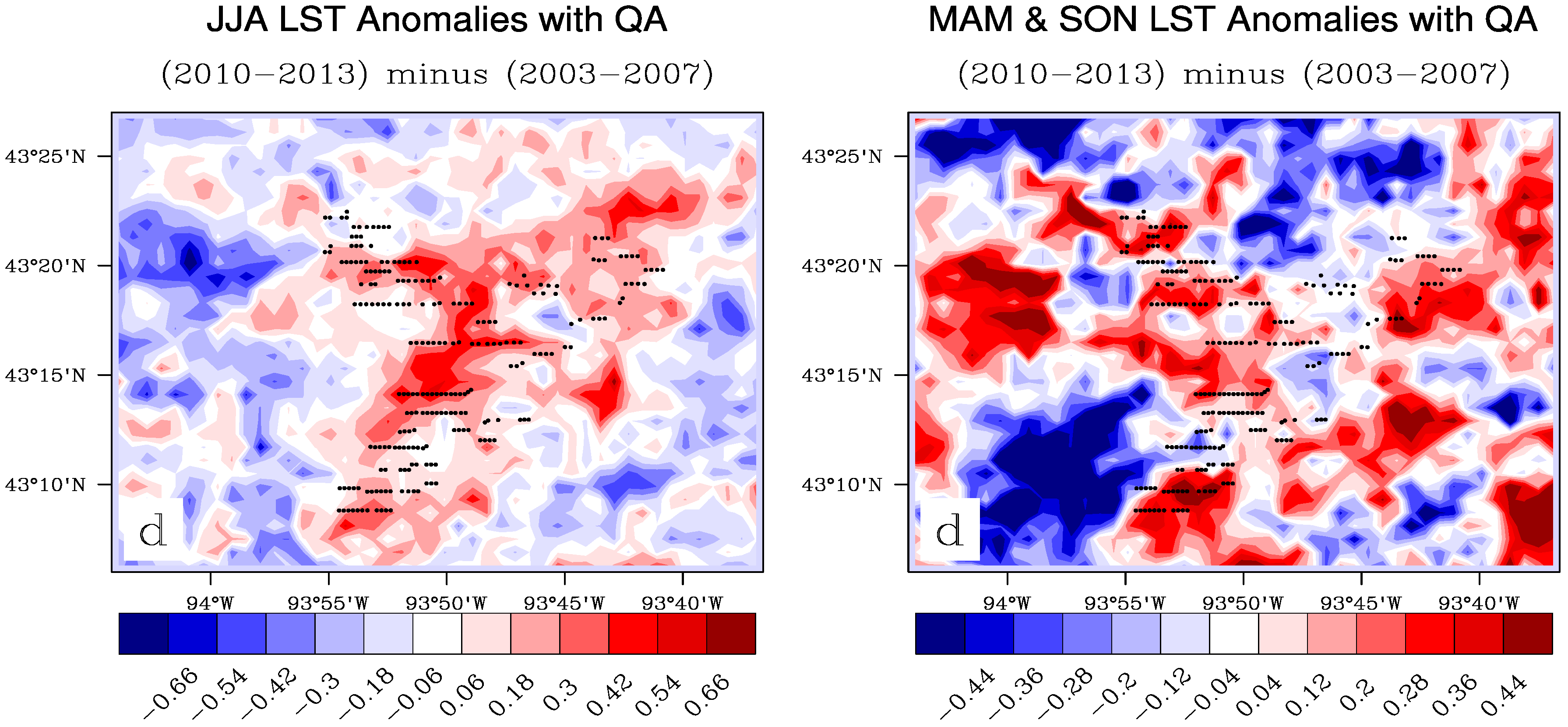Figure 6 uses WF d, the one from this study with the most turbines, as an example for plotting pixel-level LST anomaly differences using only the highest quality data. It demonstrates that the WF-warming signals at ~10:30 p.m. are robust when using different QA criteria, and it supports the conclusion from previous figures that JJA is the best season for detecting such a signal. Table 3 is the same as Table 2, except it uses three different sets of QA criteria. WFs b and c have negative values with various QA criteria, and as described before, the negative values do not necessarily indicate a WF-cooling effect.

Figure 6. Pixel-level anomaly differences for WF d for JJA (left) and MAM and SON (right), at ~10:30 p.m., with quality assurance criteria only allowing for pixels with the best quality.

Figure 6. Pixel-level anomaly differences for WF d for JJA (left) and MAM and SON (right), at ~10:30 p.m., with quality assurance criteria only allowing for pixels with the best quality.

Table 3. Mean WFP-NNWFP LST anomaly differences at ~10:30 p.m. for each WF, using the following quality assurance criteria: only the best quality pixels (QA), any quality pixels with LST errors ≤ 1 K (QA 1), and any quality pixels with LST errors ≤ 2 K (QA 2).

QA	a	b	c	d	e
MAM	0.086	−0.288	0.198	0.046	0.296
JJA	0.148	0.175	0.099	0.268	0.171
SON	0.079	0.203	−0.255	0.264	0.474
QA 1	a	b	c	d	e
MAM	0.086	−0.286	0.198	0.048	0.296
JJA	0.148	0.175	0.099	0.268	0.171
SON	0.079	0.203	−0.255	0.264	0.474
QA 2	a	b	c	d	e
MAM	0.036	−0.093	0.174	0.213	0.467
JJA	0.184	0.227	0.119	0.143	0.259
SON	0.202	0.179	0.181	0.238	0.471

Table 3. Mean WFP-NNWFP LST anomaly differences at ~10:30 p.m. for each WF, using the following quality assurance criteria: only the best quality pixels (QA), any quality pixels with LST errors ≤ 1 K (QA 1), and any quality pixels with LST errors ≤ 2 K (QA 2).

QA	a	b	c	d	e
MAM	0.086	−0.288	0.198	0.046	0.296
JJA	0.148	0.175	0.099	0.268	0.171
SON	0.079	0.203	−0.255	0.264	0.474
QA 1	a	b	c	d	e
MAM	0.086	−0.286	0.198	0.048	0.296
JJA	0.148	0.175	0.099	0.268	0.171
SON	0.079	0.203	−0.255	0.264	0.474
QA 2	a	b	c	d	e
MAM	0.036	−0.093	0.174	0.213	0.467
JJA	0.184	0.227	0.119	0.143	0.259
SON	0.202	0.179	0.181	0.238	0.471

The lack of signal in DJF suggests that the overall wintertime ABL in Iowa is not favorable for allowing WF impacts to be observed with these methods, presumably because the near-surface ABL characteristics and land surface properties in winter are dramatically different from other seasons. In contrast, the negative values in MAM for WF b and SON for WF c suggest that the ABL conditions in those particular regions are not favorable for observable WF impacts in those seasons, rather than the problem being specific to those seasons in general.

All seasons and MODIS measurement times were examined for WF impacts, and a nighttime warming was observed. An opposite scenario for daytime cooling was not observed for any WF, likely because enhanced mixing from turbines would have very little effect on a typical daytime ABL that is turbulent and already well-mixed (i.e., $\text{∂θ}/\text{∂z}$ ~ 0) [3,9]. MODIS LST changes at ~1:30 a.m. were also examined, and warming signals were found to be smaller and less spatially coupled than those at ~10:30 p.m. (figures not shown). Consistent with Zhou et al. [13], the results for each WF were better in JJA than in other seasons, and at ~10:30 p.m. than later in the nighttime at ~1:30 a.m. These results raise new questions about the differences in the nocturnal ABL between the ~10:30 p.m. and ~1:30 a.m. MODIS measurement times, and how such differences affect WF impacts. The nocturnal ABL can be complex and difficult to diagnose or predict due to night-to-night variability in turbulent and radiative cooling processes [22,23,24]. These questions will be addressed in future work using observational data from tall towers.

Zhou et al. [14] determined that their observed WF warming signals were not an artifact of the topography. The topography over the WFs in this study, which is fairly flat relative to the terrain on which the Texas WFs are built, did not appear to have any effect on the LST anomaly differences. Zhou et al. [12] determined that small changes in land surface properties could not account for the warming signals that they observed over WF pixels. No significant changes in land surface properties were noticed over the WF regions in this study, so the nighttime warming signals shown in these results are very likely caused by operational wind turbines. The WF-warming signal magnitudes observed here are slightly smaller than the magnitudes observed in Zhou et al. [13]. This discrepancy is likely due to ABL differences between the semi-arid Texas grasslands and the Iowa farmlands, as those two land surface types have disparate surface sensible and latent heat fluxes [15]. The Texas WFs are grouped together and have more turbines than all of the Iowa WFs. The number of turbines in this study ranges from 76 to 224 (Table 1), whereas the total number of turbines investigated by Zhou et al. [12,13,14] was 2358. Lu and Porté-Agel [8] noted that different turbine spacing can cause different WF effects on ABL turbulence intensity, so the smaller number of turbines and different spacing in the Iowa WFs could contribute to the smaller magnitudes of the warming signals as well.

4. Conclusions

Observing local WF impacts is important because of the potential impacts of large-scale wind power use on global climate [25,26,27]. For WFs built on croplands, their impacts on local meteorology also have implications for agriculture, as vertical fluxes of heat, moisture, CO2, and momentum can have an effect on crop growth [11]. Different parameterizations of WFs in models do not always agree [28], so understanding observed WF impacts can help improve model representations of WFs. Using two different methods and eleven years of MODIS LST data, this study has provided evidence of WF-induced surface warming at nighttime over five individual WFs in Iowa. This effect has been predicted by several previous studies and observed by a few. The same dataset and methodology as Zhou et al. [13] were used here, but for other locations with different topography and different land surface properties. The results presented here agree with their results, showing that the WF warming signal is not unique to their study region. The nighttime WF-warming signals occur in each season except DJF, which creates a discrepancy between this study and Zhou et al. [13], likely due to the differences in land surface properties and local climate. The best signal occurs in JJA at ~10:30 p.m., in agreement with Zhou et al. [13]. Seemingly, the ABL characteristics and land surface properties in summertime at about 10 p.m. are the most favorable for allowing such WF impacts to be observed with the given data and methodology.