Application of In-Segment Multiple Sampling in Object-Based Classification

Abstract
:
1. Introduction
- -
- To describe in-segment pixel heterogeneity by exploiting the potential of multiple small set sampling,
- -
- To study the effect of multiple small set sampling on normality violation with the parametric Student’s t-test,
- -
- To compare the effectiveness of the Kolmogorov-Smirnov and Student’s t-test based classifiers, and
- -
- To analyze the impact spectral resolution has on the classification results.
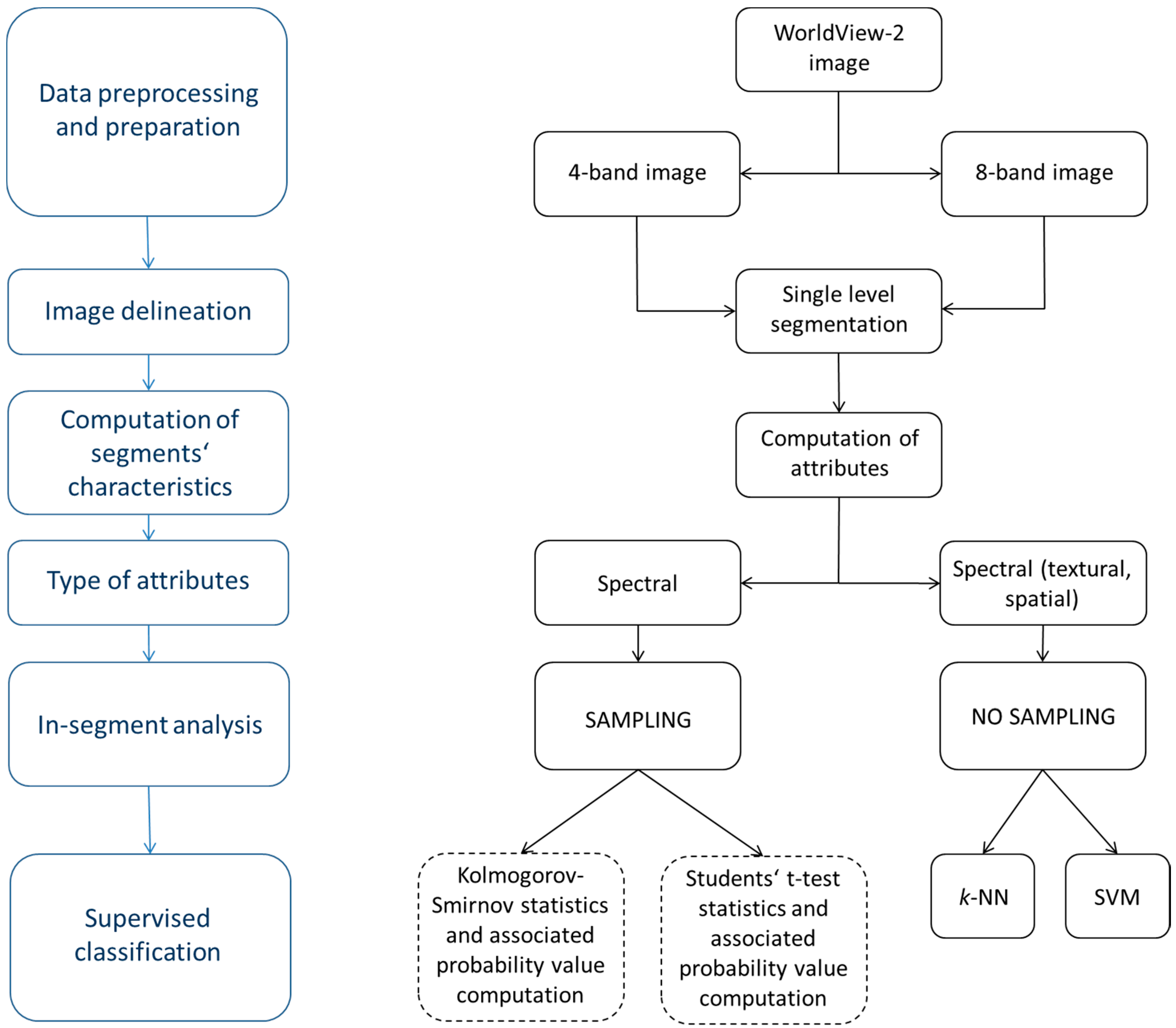
2. Data and Methodology
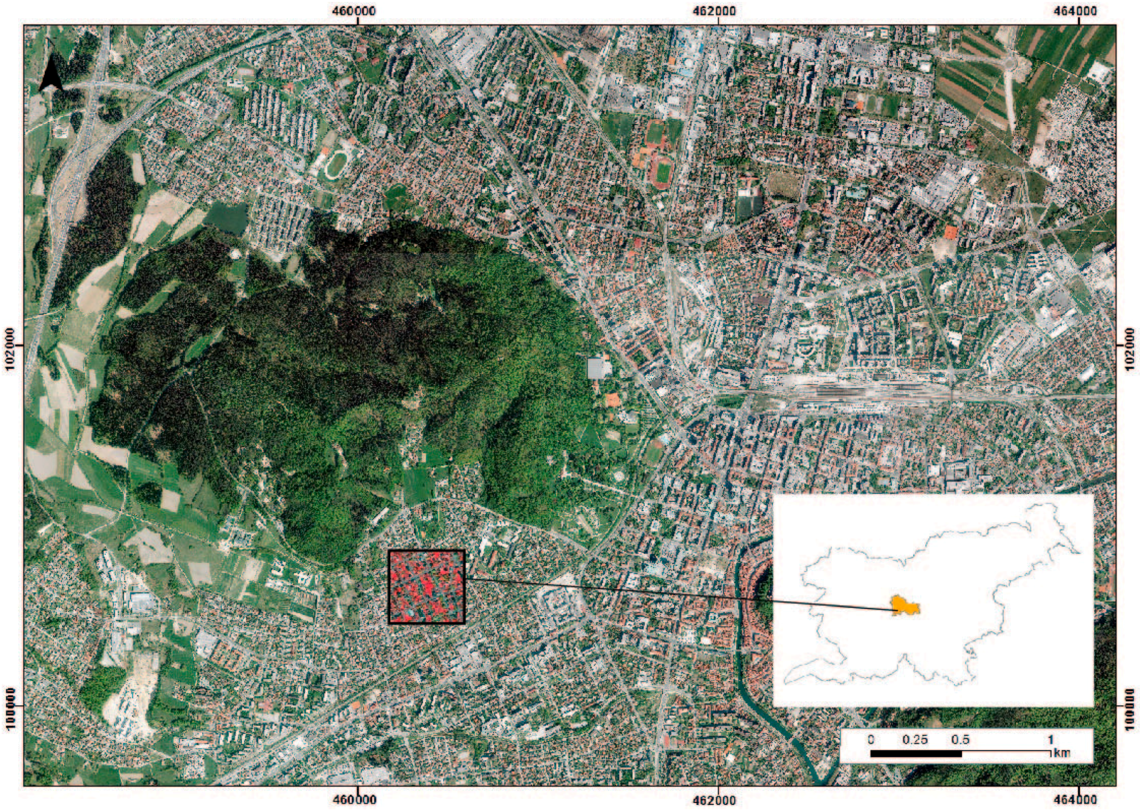
2.1. Case Study Area and Data

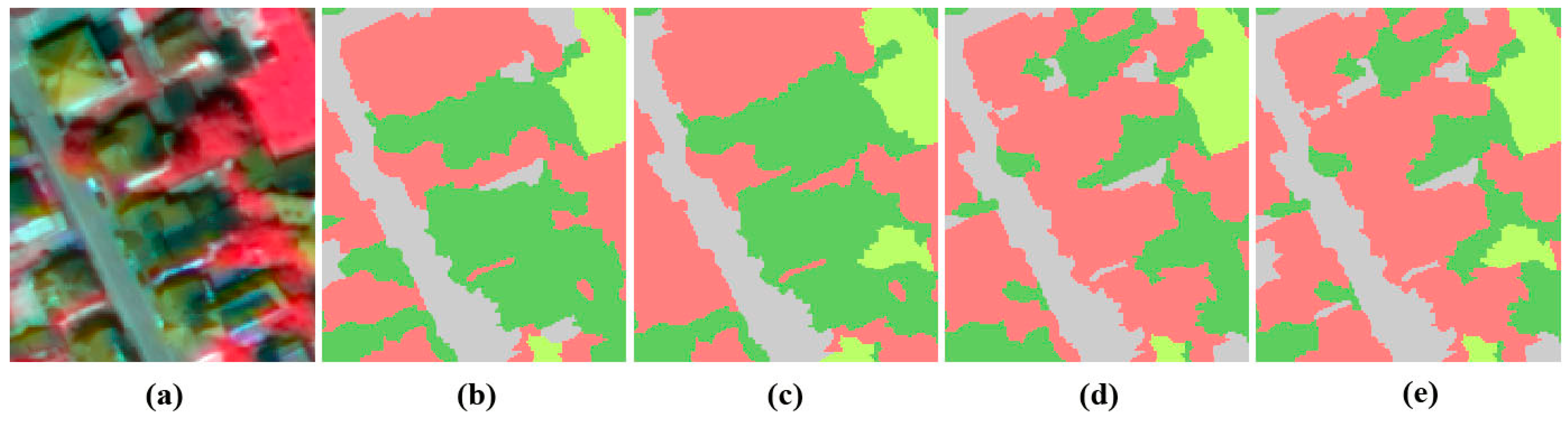
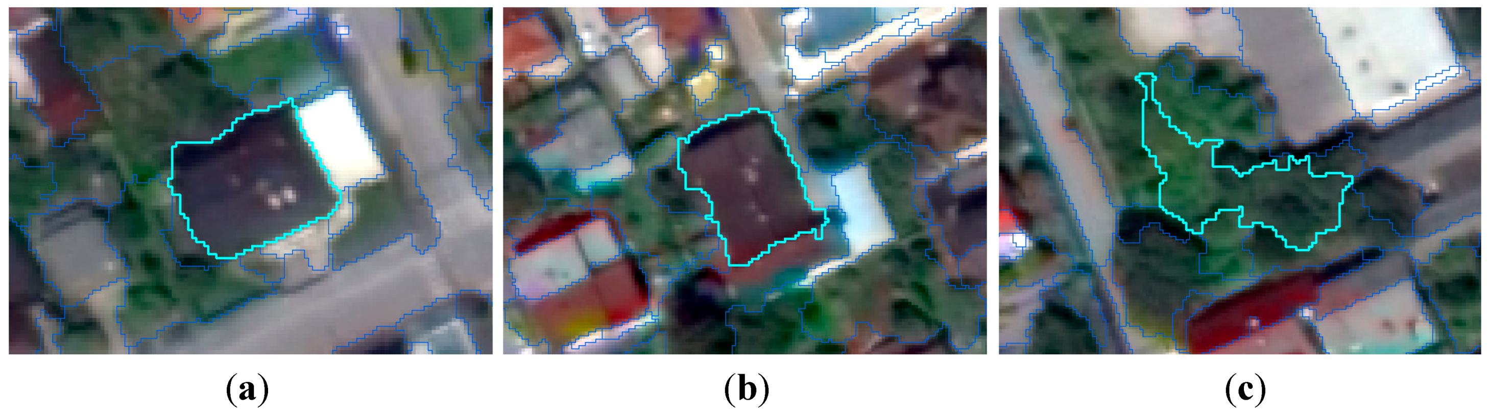
2.2. Segmentation
2.3. The Selection of Training and Testing Samples

| Attribute | Type | Description |
|---|---|---|
| Spectral | Minimum | Minimum value of pixels comprising the region in band x. |
| Maximum | Maximum value of pixels comprising the region in band x. | |
| Mean | Mean value of pixels comprising the region in band x. | |
| Standard deviation | Standard deviation value of pixels comprising the region in band x. | |
| Texture | Range | Average data range of pixels comprising the region within the kernel. |
| Mean | Average value of pixels comprising the region within the kernel. | |
| Variance | Average variance of pixels comprising the region within the kernel. | |
| Entropy | Average entropy value of pixels comprising the region within the kernel. | |
| Spatial | Area | Total area of the polygon, minus the area of the holes. |
| Length | The combined length of all polygon boundaries, including the boundaries of the holes. | |
| Compactness | A shape measurement that indicates the compactness of the polygon. A circle is the most compact shape with a value of 1/π. | |
| Convexity | This attribute measures the convexity of the polygon. The convexity value for a convex polygon with no holes is 1.0, while the value for a concave polygon is below 1.0. | |
| Solidity | A shape measurement that compares the area of the polygon to the area of a convex hull that surrounds the polygon. The solidity value for a convex polygon with no holes is 1.0, while the value for a concave polygon is below 1.0. | |
| Roundness | A shape measurement that compares the area of the polygon to the square of the maximum diameter of the polygon. The roundness value of a circle is 1, while the value for a square is 4/π. | |
| Form factor | A shape measurement that compares the area of the polygon to the square of the total perimeter. The form factor value of a circle is 1, while the value of a square is π/4. | |
| Elongation | A shape measurement that indicates the ratio of the major axis of the polygon to the minor axis of the polygon. The elongation value for a square is 1.0, while the value for a rectangle is greater than 1.0. | |
| Rectangular fit | A shape measurement that indicates how well the shape is described by a rectangle. The rectangular fit value for a rectangle is 1.0, while the value for a non-rectangular shape is below 1.0. | |
| Main direction | The angle subtended by the major axis of the polygon and the x-axis in degrees. The main direction value ranges between 0 and 180°. 90° is North/South, while 0 to 180° is East/West. | |
| Major length | The length of the major axis of an oriented bounding box that encloses the polygon. | |
| Minor length | The length of the minor axis of an oriented bounding box that encloses the polygon. | |
| Number of holes | The number of holes in the polygon. | |
| Hole area | The ratio of the total area of the polygon towards the area of the outer contour of the polygon. The hole-solid ratio value for a polygon with no holes is 1.0. |
| Class | Number of Selected Segments for Training Samples | Number of Selected Segments for Testing Samples |
|---|---|---|
| Roads | 6 | 67 |
| Buildings | 11 | 257 |
| Trees | 7 | 176 |
| Grass | 5 | |
| Total | 29 | 500 |
2.4. Supervised Classification Process
2.4.1. The Two-Sample Kolmogorov-Smirnov Test Statistics Based Classification Algorithm
2.4.2. Student’s t-Test Statistics Based Classification Algorithm
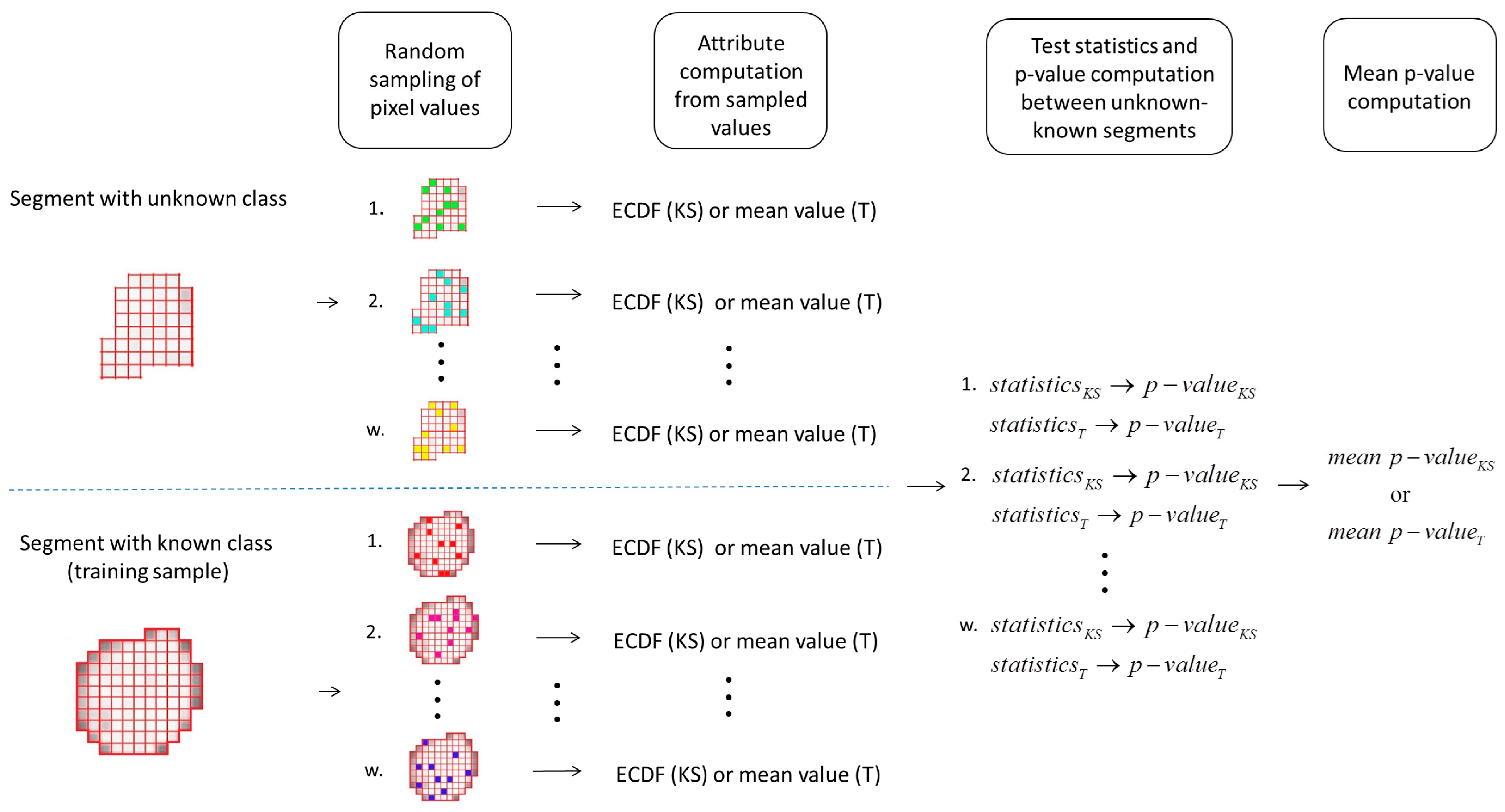
2.4.3. Random Sampling Approach
3. Results and Discussion
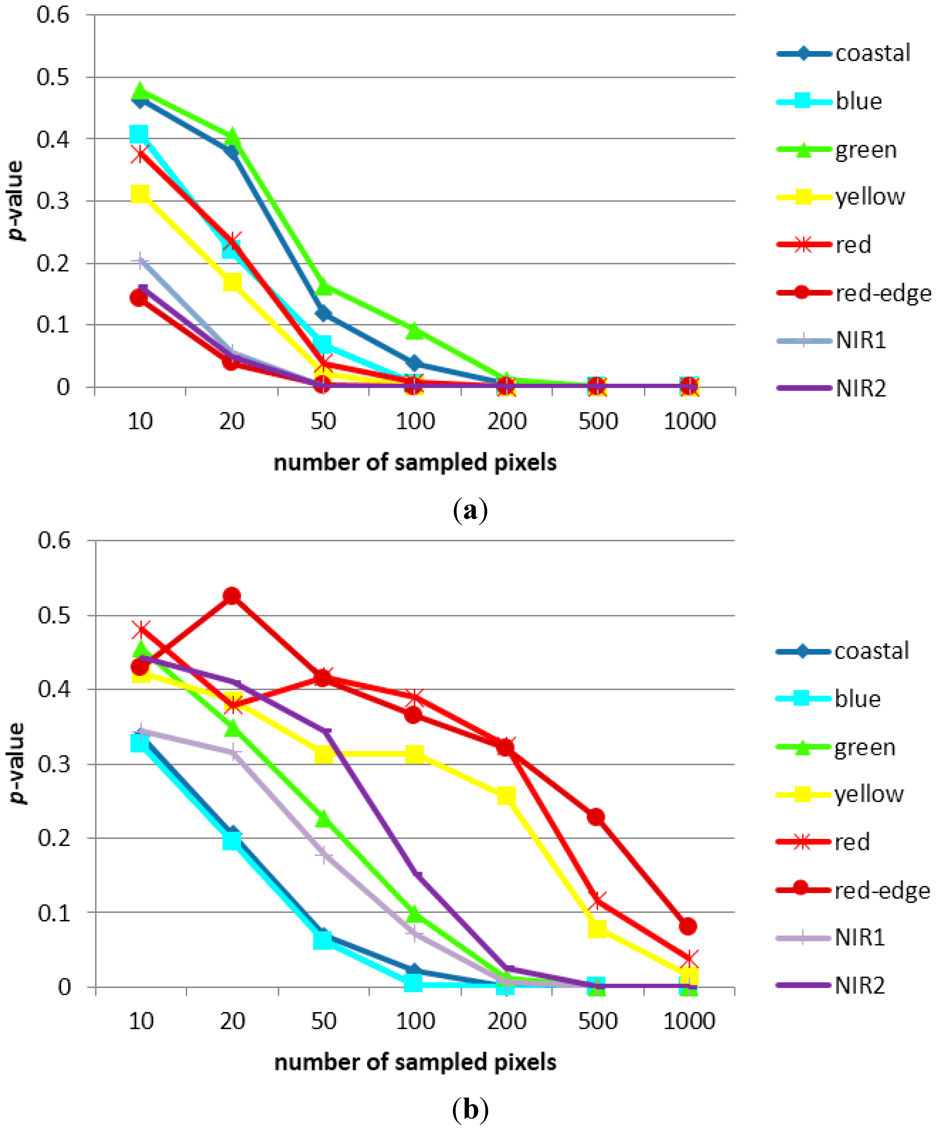
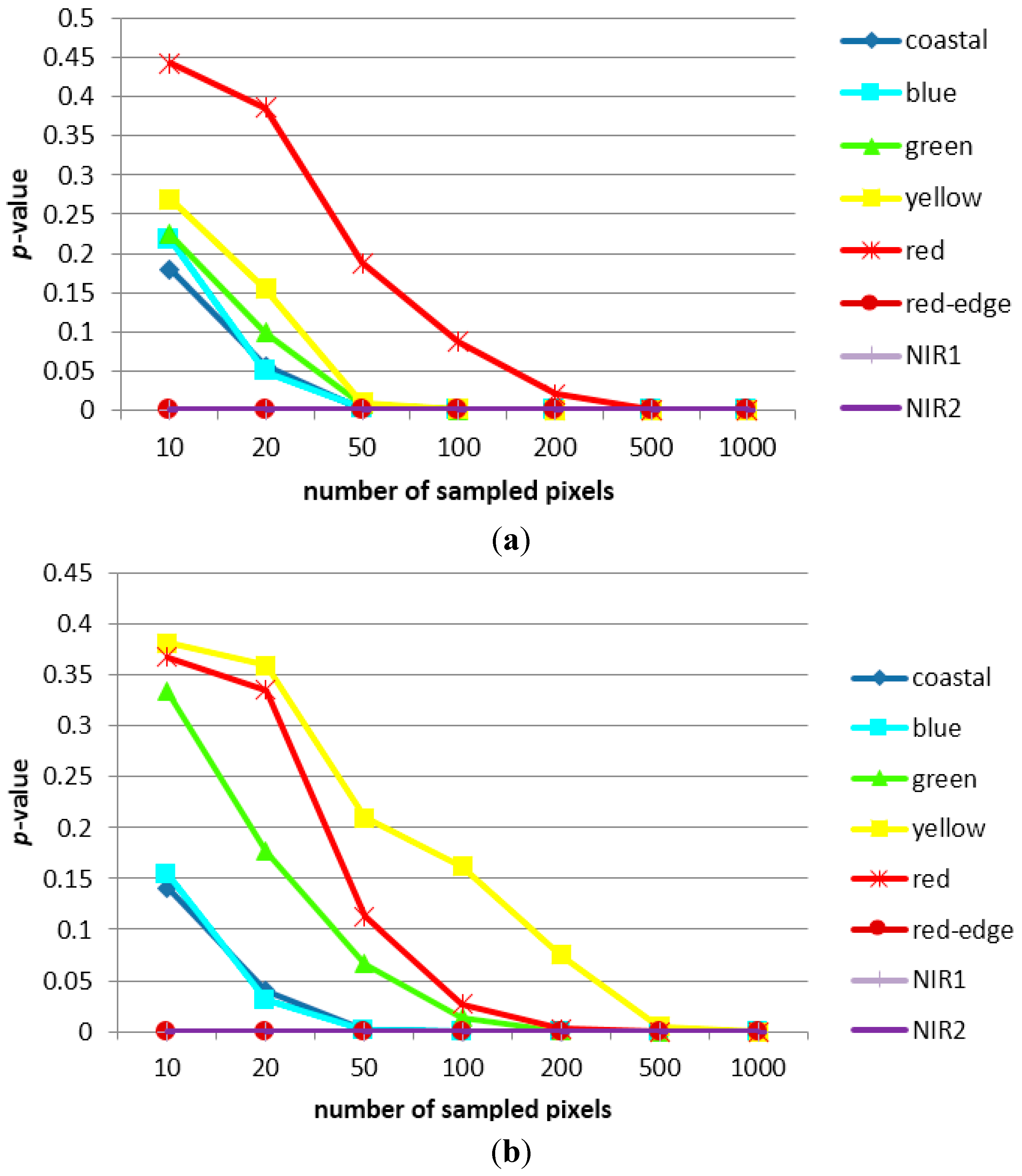
3.1. Sampling Analysis
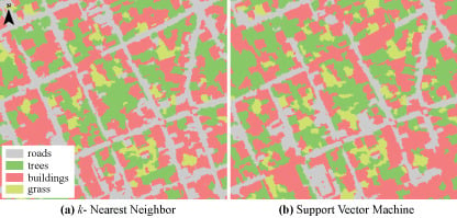
3.2. Classification Results and Accuracy Assessment
| k-Nearest Neighbor | ||||||||||
| 4-Band Image | 8-Band Image | |||||||||
| Reference | Roads | Building | Trees + Grass | Total | Producer Accuracy (%) | Roads | Building | Trees + Grass | Total | Producer Accuracy (%) |
| Roads | 43 | 20 | 4 | 67 | 59.7 | 48 | 18 | 1 | 67 | 57.8 |
| Building | 29 | 190 | 38 | 257 | 87.6 | 32 | 195 | 30 | 257 | 82.2 |
| Trees + grass | 0 | 7 | 169 | 176 | 80.1 | 3 | 24 | 149 | 176 | 82.8 |
| Total | 72 | 217 | 211 | 500 | 75.8 | 83 | 237 | 180 | 500 | 74.3 |
| User accuracy (%) | 64.2 | 73.9 | 96.0 | 78.0 | 71.6 | 75.9 | 84.6 | 77.4 | ||
| Support Vector Machine | ||||||||||
| 4-Band Image | 8-Band Image | |||||||||
| Reference | Roads | Building | Trees + Grass | Total | Producer Accuracy (%) | Roads | Building | Trees + Grass | Total | Producer Accuracy (%) |
| Roads | 22 | 41 | 4 | 67 | 59.5 | 23 | 18 | 1 | 67 | 62.2 |
| Building | 15 | 210 | 32 | 257 | 83.3 | 13 | 210 | 34 | 257 | 90.5 |
| Trees + grass | 0 | 1 | 175 | 176 | 82.9 | 1 | 4 | 171 | 176 | 83.0 |
| Total | 37 | 252 | 211 | 500 | 75.2 | 37 | 232 | 206 | 500 | 78.6 |
| User accuracy (%) | 32.8 | 81.7 | 99.4 | 71.3 | 34.3 | 81.7 | 97.1 | 71.0 | ||
| Two-Sample Kolmogorov-Smirnov Test Statistics Classifier | ||||||||||
| 4-Band Image | 8-Band Image | |||||||||
| Reference | Roads | Building | Trees + Grass | Total | Producer Accuracy (%) | Roads | Building | Trees + Grass | Total | Producer Accuracy (%) |
| Roads | 52 | 14 | 1 | 67 | 61.1 | 52 | 14 | 1 | 67 | 59.0 |
| Building | 33 | 179 | 45 | 257 | 92.7 | 36 | 181 | 40 | 257 | 92.8 |
| Trees + grass | 0 | 0 | 176 | 176 | 79.3 | 0 | 0 | 176 | 176 | 81.1 |
| Total | 85 | 193 | 222 | 500 | 77.7 | 88 | 195 | 217 | 500 | 77.6 |
| User accuracy (%) | 77.6 | 69.6 | 100 | 82.4 | 77.6 | 70.4 | 100 | 82.7 | ||
| Student’s t-Test Statistics Classifier | ||||||||||
| 4-Band Image | 8-Band Image | |||||||||
| Reference | Roads | Building | Trees + Grass | Total | Producer Accuracy (%) | Roads | Building | Trees + Grass | Total | Producer Accuracy (%) |
| Roads | 52 | 14 | 1 | 67 | 56.5 | 52 | 14 | 1 | 67 | 59.1 |
| Building | 40 | 194 | 23 | 257 | 93.3 | 36 | 196 | 25 | 257 | 93.3 |
| Trees + grass | 0 | 0 | 176 | 176 | 88.0 | 0 | 0 | 176 | 176 | 871 |
| Total | 92 | 208 | 200 | 500 | 79.3 | 88 | 210 | 202 | 500 | 79.8 |
| User accuracy (%) | 77.6 | 75.5 | 100 | 84.4 | 77.6 | 75.5 | 100 | 84.4 | ||
| k-Nearest Neighbor | ||||||||||
| 4-Band Image | 8-Band Image | |||||||||
| Reference | Roads | Building | Trees + Grass | Total | Producer Accuracy (%) | Roads | Building | Trees + Grass | Total | Producer Accuracy (%) |
| Roads | 40 | 20 | 7 | 67 | 68.9 | 44 | 20 | 3 | 67 | 74.6 |
| Building | 16 | 202 | 39 | 257 | 83.1 | 14 | 213 | 30 | 257 | 81.9 |
| Trees/grass | 2 | 21 | 153 | 176 | 76.9 | 1 | 27 | 148 | 176 | 81.8 |
| Total | 58 | 243 | 199 | 500 | 76.3 | 59 | 260 | 181 | 500 | 79.4 |
| User accuracy (%) | 59.7 | 78.6 | 86.9 | 75.1 | 65.7 | 82.9 | 84.1 | 77.6 | ||
| Support Vector Machine | ||||||||||
| 4-Band Image | 8-Band Image | |||||||||
| Reference | Roads | Building | Trees + Grass | Total | Producer Accuracy (%) | Roads | Building | Trees + Grass | Total | Producer Accuracy (%) |
| Roads | 32 | 25 | 10 | 67 | 88.9 | 35 | 30 | 2 | 67 | 87.5 |
| Building | 4 | 226 | 27 | 257 | 87.9 | 5 | 231 | 21 | 257 | 87.1 |
| Trees/grass | 0 | 6 | 170 | 176 | 82.1 | 0 | 4 | 172 | 176 | 88.2 |
| Total | 36 | 257 | 207 | 500 | 86.3 | 40 | 265 | 195 | 500 | 87.6 |
| User accuracy (%) | 47.8 | 87.9 | 96.6 | 77.4 | 52.2 | 89.9 | 97.7 | 79.9 | ||

4. Conclusions
Acknowledgments
Author Contributions
Conflicts of Interest
References
- Baraldi, A.; Boschetti, L. Operational automatic remote sensing image understanding systems: beyond Geographic Object-Based and Object-Oriented Image Analysis (GEOBIA/GEOOIA). Part 1: Introduction. Remote Sens. 2012, 4, 2694–2735. [Google Scholar] [CrossRef]
- Blaschke, T. Object based image analysis for remote sensing. ISPRS J. Photogramm. Remote Sens. 2010, 65, 2–16. [Google Scholar] [CrossRef]
- Arvor, D.; Durieux, L.; Andrés, S.; Laporte, M-A. Advances in geographic object-based image analysis with ontologies: A review of main contributions and limitations from a remote sensing perspective. ISPRS J. Photogramm. Remote Sens. 2013, 82, 125–137. [Google Scholar] [CrossRef]
- Dos Santos, J.A. Semi-Automatic Classification of Remote Sensing Images. Ph.D. Thesis, Universidade Estadual de Campinas, Campinas, Brasil, 30 April 2013. [Google Scholar]
- Qian, J.; Zhou, Q.; Hou, Q. Comparison of pixel-based and object-oriented classification methods for extracting built-up areas in Aridzone. In Proceedings of the 2007 ISPRS Workshop on Updating Geo-Spatial Databases with Imagery & The 5th ISPRS Workshop on Dynamic and Multi-Dimensional GIS, Urumchi, China, 28–29 August 2007.
- Kressler, F.P.; Steinnocher, K.; Franzen, M. Object-oriented classification of orthophotos to support update of spatial databases. In Proceedings of the 2005 IEEE International Geoscience and Remote Sensing Symposium, Seoul, Korea, 25–29 July 2005; pp. 253–256.
- Marpu, P.R.; Neubert, M.; Herold, H.; Niemeyer, I. Enhanced evaluation of image segmentation results. J. Spat. Sci. 2010, 55, 55–68. [Google Scholar] [CrossRef]
- Sridharan, H.; Qiu, F. Developing an object-based hyperspatial image classifier with a case study using WorldView-2 data. Photogramm. Eng. Remote Sens. 2013, 79, 1027–1036. [Google Scholar] [CrossRef]
- Lübcker, T.; Schaab, G. Optimization of parameter settings for multilevel image segmentation in Geobia. In Proceedings of the 2009 ISPRS Hannover Workshop High-Resolution Earth Imaging for Geospatial Information, Hannover, Germany, 2–5 June 2009.
- Li, C.; Wang, J.; Wang, L.; Hu, L.; Gong, P. Comparison of classification algorithms and training sample sizes in urban land classification with Landsat thematic mapper imagery. Remote Sens. 2014, 6, 964–983. [Google Scholar] [CrossRef]
- Toure, S.; Stow, D.A.; Weeks, J.R.; Kumar, S. Histogram curve matching approaches for object-based image classification of land cover and land use. Photogramm. Eng. Remote Sens. 2013, 79, 433–440. [Google Scholar] [CrossRef]
- Đurić, N.; Pehani, P.; Oštir, K. The within and between segment separability analysis of sealed urban land use classes. In Proceedings of the 2013 Simpósio Brasileiro de Sensoriamento Remoto, Foz do Iguaçu, PR, Brasil, 13–18 April 2013; pp. 2392–2399.
- Pal, N.R.; Pal, S.K. A review on image segmentation techniques. Pattern Recognit. 1993, 26, 1277–1294. [Google Scholar] [CrossRef]
- </b>Mesner, N.; Oštir, K. Investigating the impact of spatial and spectral resolution of satellite images on segmentation quality. J. Appl. Remote Sens. 2014, 8, 083696. [Google Scholar] [CrossRef]
- Lizarazo, I.; Elsner, P. Improving urban land cover classification using fuzzy image segmentation. Lect. Notes Comput. Sci. 2009, 5730, 41–56. [Google Scholar]
- List of Attributes. Available online: http://www.exelisvis.com/docs/AttributeList.html (accessed on 19 August 2014).
- K Nearest Neighbor Background. Available online: http://www.exelisvis.com/docs/BackgroundKNN.html (accessed on 20 August 2014).
- Support Vector Machine Background. Available online: http://www.exelisvis.com/docs/BackgroundSVM.html (accessed on 21 August 2014).
- Tzotsos, A. A support vector machine approach for object based image analysis. In Bridging Remote Sensing and GIS, Proceedings of the 2006 International Conference on Object-based Image Analysis, Salzburg, Austria, 4–5 July 2006.
- Gibbons, J.D.; Chakraborti, S. Nonparametric Statistical Interference, 4th ed.; Marcel Dekker Inc.: New York, NY, USA, 2003; p. 37. [Google Scholar]
- Wang, H. Stochastic Modelling of the Equilibrium Speed-Density Relationship. Ph.D. Thesis, University of Massachusetts Amherst, Amherst, MA, USA, 1 September 2010. [Google Scholar]
- Gordon, A.Y.; Klebanov, L.B. On a paradoxical property of the Kolmogorov-Smirnov two-sample tes. In Nonparametrics and Robustness in Modern Statistical Inference and Time Series Analysis: A Festschrift in Honor of Professor Jana Jurečková; Antoch, J., Hušková, M., Sen, P.K., Eds.; Institute of Mathematical Statistics: Beachwood, OH, USA, 2010; Volume 7, pp. 70–74. [Google Scholar]
- Arcidiacono, C.; Porto, S.M.C.; Cascone, G. Accuracy of crop-shelter thematic maps: A case study of maps obtained by spectral and textural classification of high-resolution satellite image. J. Food Agric. Environ. 2012, 10, 1071–1074. [Google Scholar]
- Immitzer, M.; Atzberger, C.; Koukal, T. Tree species classification with random forest using very high spatial resolution 8-band Worldview-2 satellite data. Remote Sens. 2012, 4, 2661–2693. [Google Scholar] [CrossRef]
- Huang, C.; Davis, L.S.; Townshend, J.R.G. An assessment of support vector machines for land cover classification. Int. J. Remote Sens. 2002, 23, 725–749. [Google Scholar] [CrossRef]
- Myburgh, G.; van Niekerk, A. Effect of feature dimensionality on object-based land cover classification: A comparison of three classifiers. S. Afr. J. Geomat. 2013, 2, 13–27. [Google Scholar]
- Maillard, P.; Clausi, A.D. Pixel based sea ice classification using the MAGSIC system. In Proceedings of the 2006 ISPRS Commission VII Symposium “Remote Sensing: From Pixels to Processes”, Enschede, The Netherlands, 8–11 May 2006.
- Castilla, G.; Hay, J.G.; Ruiz-Gallardo, J. Size-constrained Region Merging (SCRM): An automated delineation tool for assisted photointerpretation. Photogramm. Eng. Remote. Sens. 2008, 74, 409–419. [Google Scholar] [CrossRef]
© 2014 by the authors; licensee MDPI, Basel, Switzerland. This article is an open access article distributed under the terms and conditions of the Creative Commons Attribution license (http://creativecommons.org/licenses/by/4.0/).
Share and Cite
Đurić, N.; Pehani, P.; Oštir, K. Application of In-Segment Multiple Sampling in Object-Based Classification. Remote Sens. 2014, 6, 12138-12165. https://doi.org/10.3390/rs61212138
Đurić N, Pehani P, Oštir K. Application of In-Segment Multiple Sampling in Object-Based Classification. Remote Sensing. 2014; 6(12):12138-12165. https://doi.org/10.3390/rs61212138
Chicago/Turabian StyleĐurić, Nataša, Peter Pehani, and Krištof Oštir. 2014. "Application of In-Segment Multiple Sampling in Object-Based Classification" Remote Sensing 6, no. 12: 12138-12165. https://doi.org/10.3390/rs61212138
APA StyleĐurić, N., Pehani, P., & Oštir, K. (2014). Application of In-Segment Multiple Sampling in Object-Based Classification. Remote Sensing, 6(12), 12138-12165. https://doi.org/10.3390/rs61212138