Delineation of Rain Areas with TRMM Microwave Observations Based on PNN

Abstract
:1. Introduction
2. Data and Method
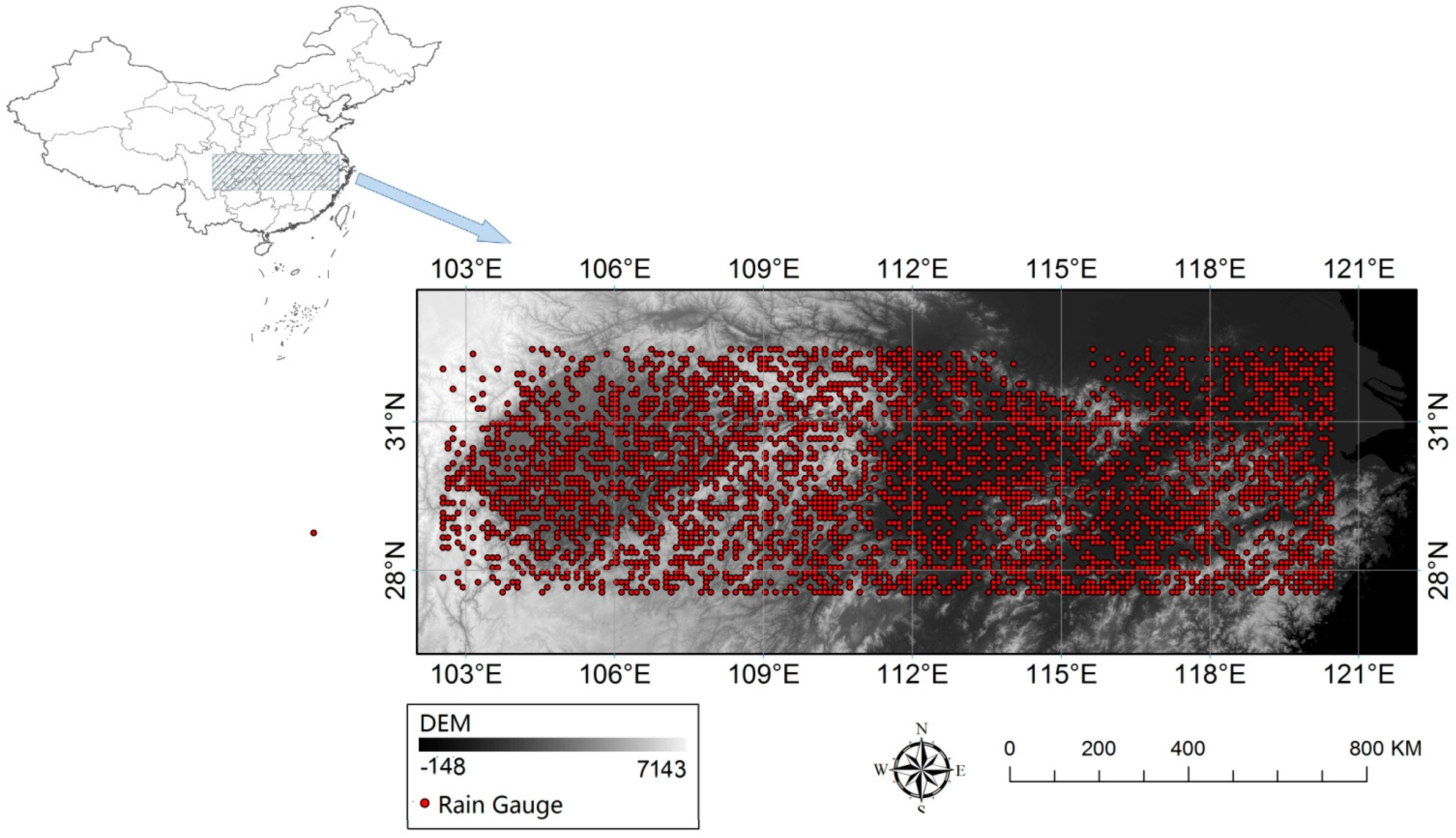
2.1. Study Area
2.2. Data
2.2.1. Rain Gauge Observations

2.2.2. Microwave Brightness Temperature Datasets
2.2.3. TRMM Microwave Imager (TMI) Level 2 Hydrometeor Profile Product
2.3. Methods
2.3.1. Scatter Index
2.3.2. Dynamic Cluster K-Means Method
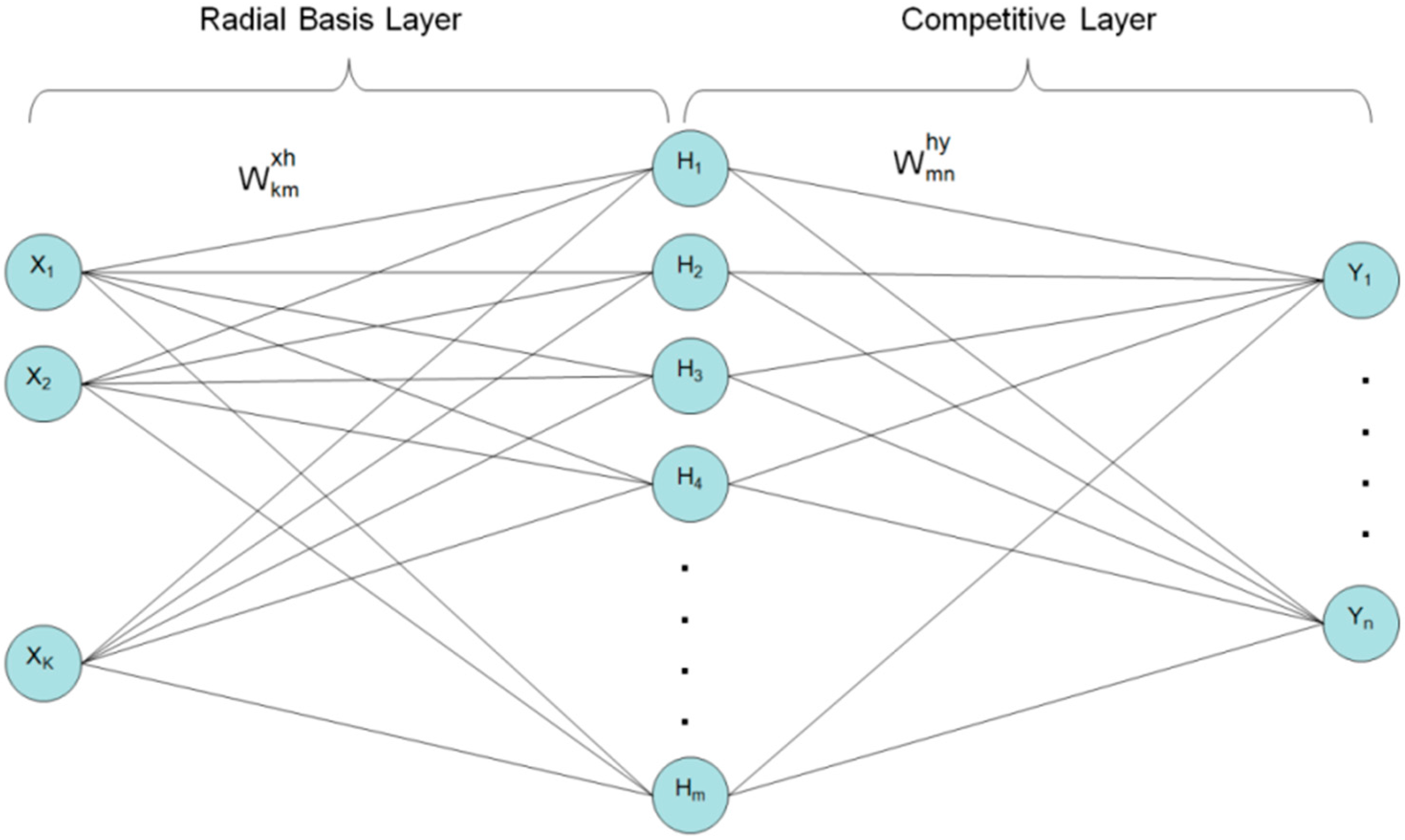
2.3.3. Brief Description of Probabilistic Neural Network
2.3.4. Rain Area Delineation Method Based on PNN
2.3.5. Validation

| Rain/No Rain Area Delineation by the Models | |||
|---|---|---|---|
| Rain | No Rain | ||
| Ground observations | Rain | h | m |
| No rain | f | z | |
3. Results
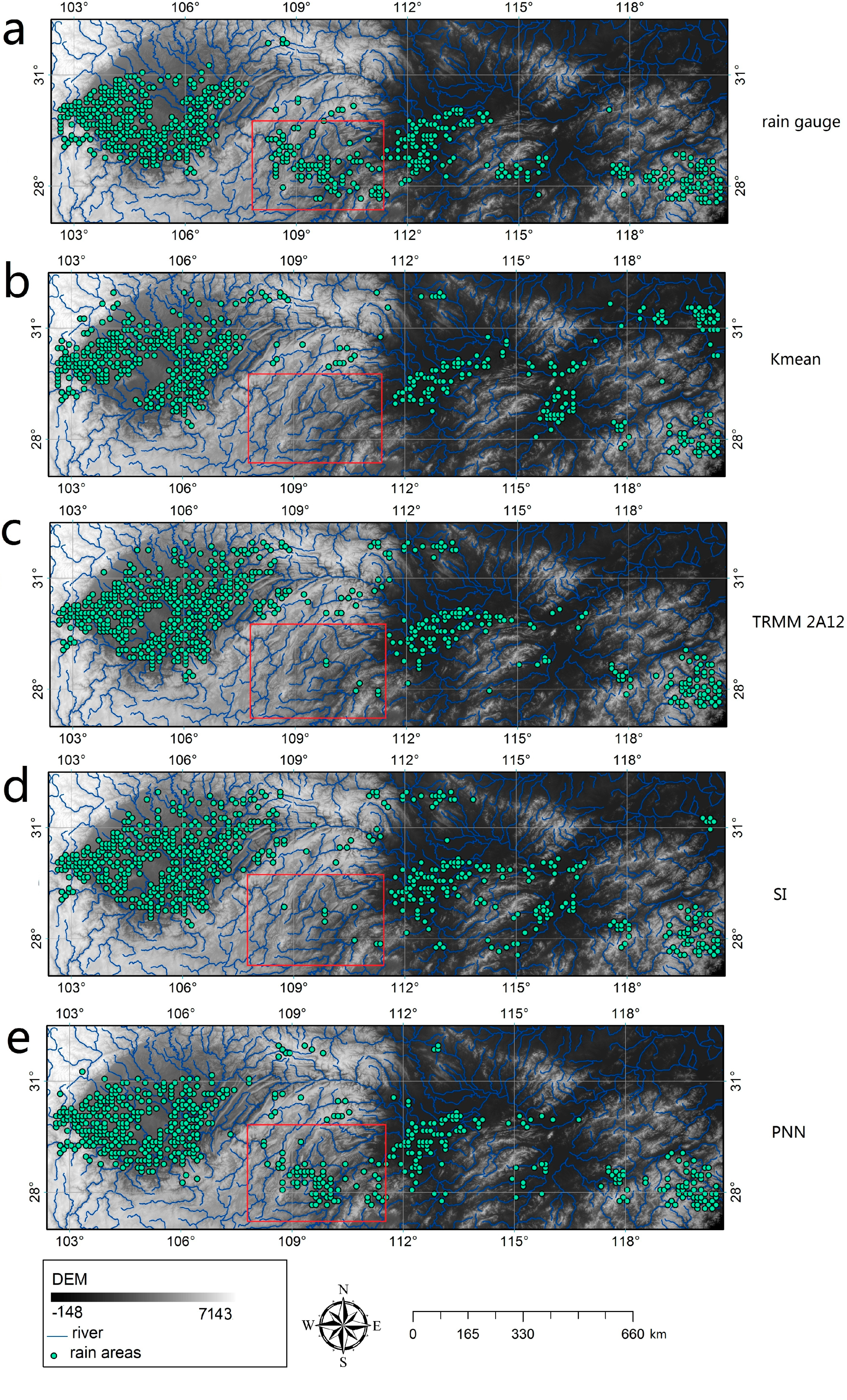
3.1. The Results of PNN and Other Rain Area Delineation Methods
| Rain Event | Time | Number of Rain Pixels | Number of No_Rain Pixels |
|---|---|---|---|
| 1 | June 25 at 2 am | 419 | 2757 |
| 2 | June 27 at 8 pm | 549 | 2607 |
| 3 | June 28 at 7 pm | 879 | 2831 |
| 4 | June 29 at 0 am | 1048 | 2286 |
| 5 | July 2 at 5 pm | 242 | 3470 |
| 6 | July 6 at 3 pm | 128 | 3518 |
| 7 | July 23 at 7 pm | 453 | 2807 |
| 8 | July 26 at 4 am | 482 | 2215 |
| 9 | July 26 at 9 am | 926 | 2662 |
| 10 | July 27 at 8 am | 483 | 2525 |
| 11 | July 29 at 3 am | 330 | 3268 |
| 12 | July 31 at 3 am | 483 | 2470 |
| 13 | August 4 at 1 am | 446 | 2646 |
| 14 | August 5 at 0 am | 317 | 2935 |
| 15 | August 5 at 5 am | 295 | 3349 |
| 16 | August 9 at 9 pm | 621 | 2297 |
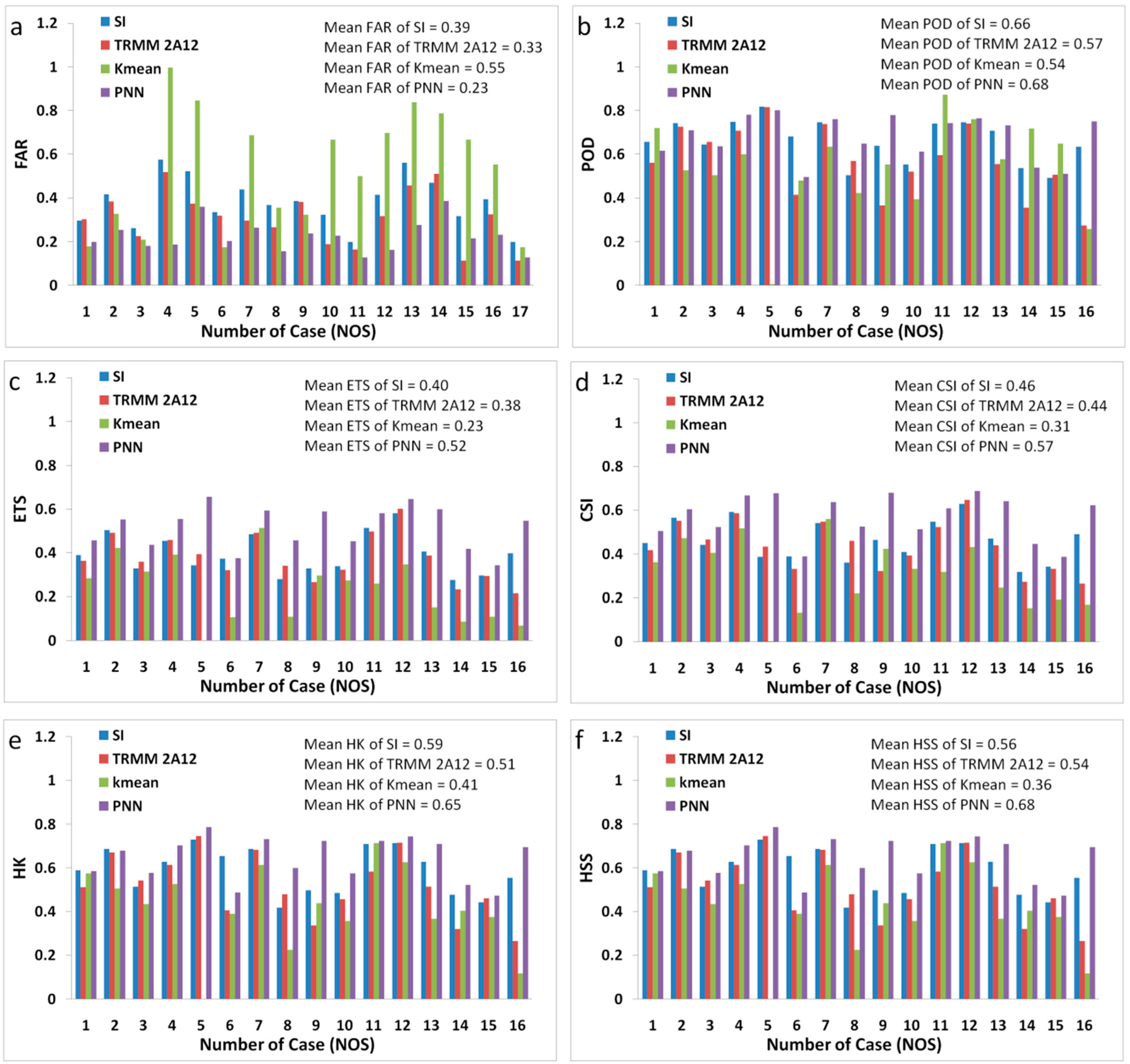
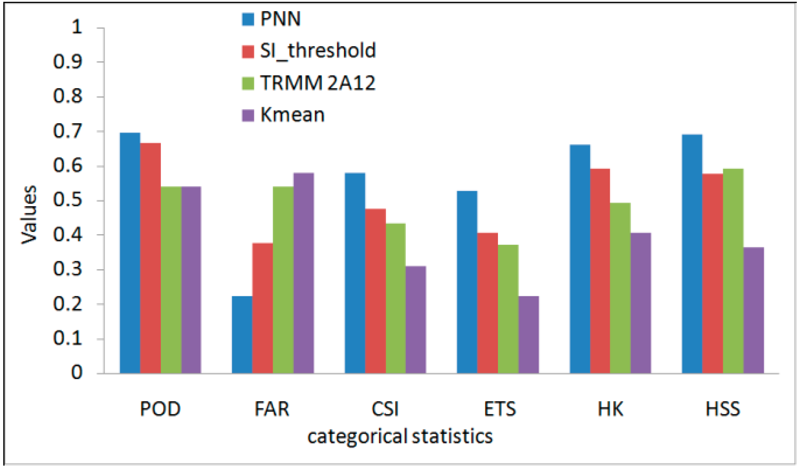
3.2. Validation and Comparison of the PNN Method
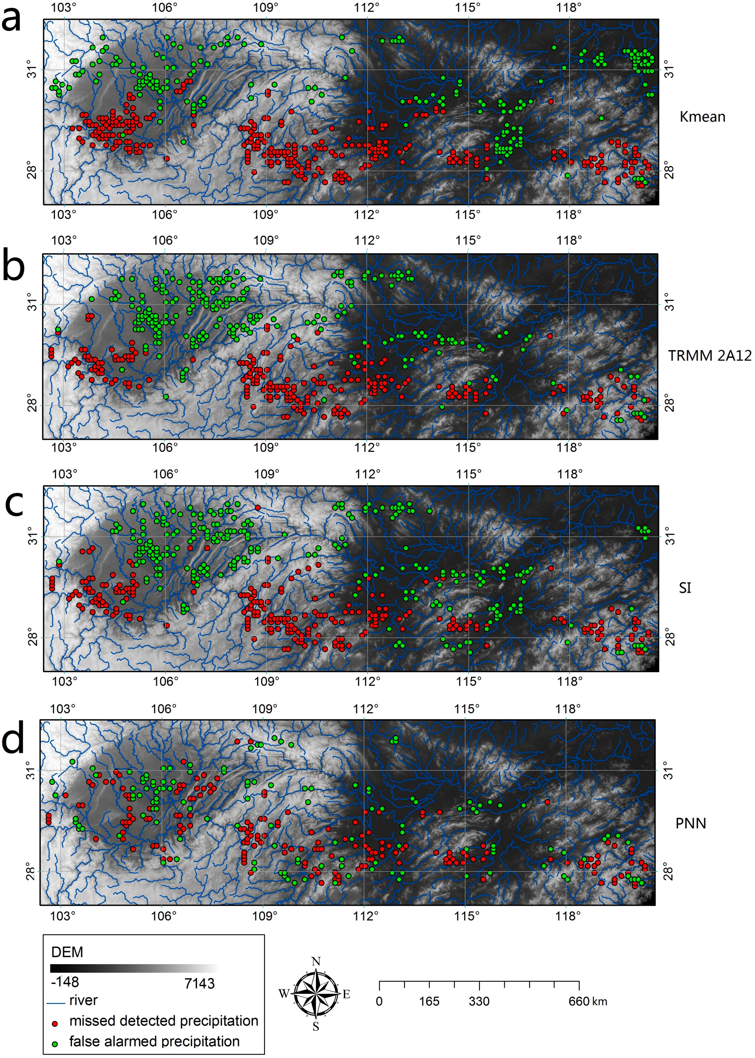


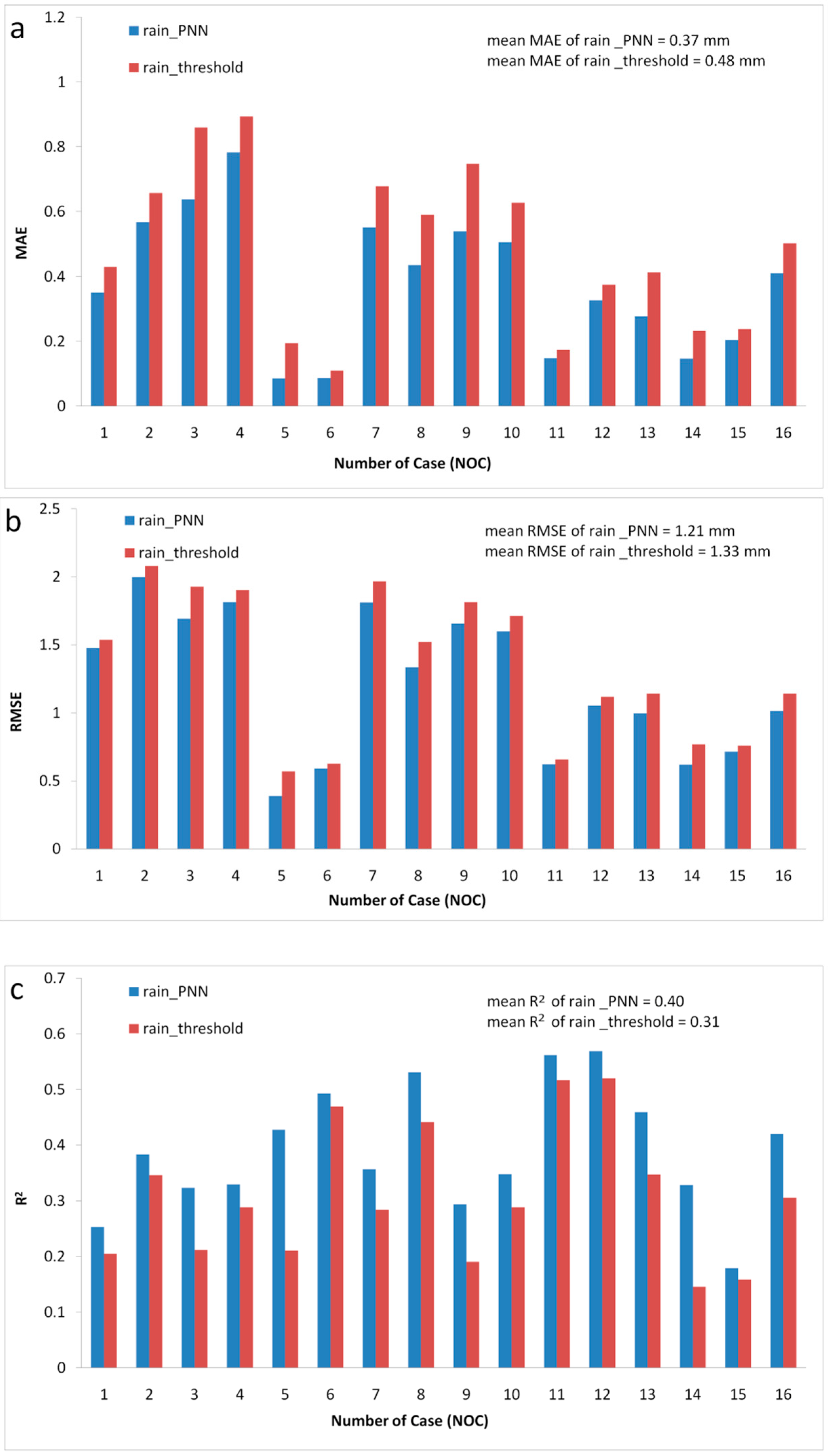
3.3. Improvement of SI with PNN Method
4. Discussion
5. Conclusions
Acknowledgments
Author Contributions
Conflicts of Interest
References
- Goovaerts, P. Geostatistical approaches for incorporating elevation into the spatial interpolation of rainfall. J. Hydrol. 2000, 228, 113–129. [Google Scholar] [CrossRef]
- Wu, C.; Chen, J.M. The use of precipitation intensity in estimating gross primary production in four northern grasslands. J. Arid Environ. 2012, 82, 11–18. [Google Scholar] [CrossRef]
- Jia, S.; Zhu, W.; Lű, A.; Yan, T. A statistical spatial downscaling algorithm of TRMM precipitation based on ndvi and dem in the qaidam basin of China. Remote Sens. Environ. 2011, 115, 3069–3079. [Google Scholar] [CrossRef]
- Xie, P.P.; Xiong, A.Y. A conceptual model for constructing high-resolution gauge-satellite merged precipitation analyses. J. Geophys. Res. Atmos. 2011, 116. [Google Scholar] [CrossRef]
- Ricciardelli, E.; Cimini, D.; Di Paola, F.; Romano, F.; Viggiano, M. A statistical approach for rain intensity differentiation using meteosat second generation-spinning enhanced visible and infrared imager observations. Hydrol. Earth Syst. Sci. 2014, 18, 2559–2576. [Google Scholar] [CrossRef]
- Mugnai, A.; Smith, E.A.; Tripoli, G.J.; Bizzarri, B.; Casella, D.; Dietrich, S.; di Paola, F.; Panegrossi, G.; Sano, P. Cdrd and pnpr satellite passive microwave precipitation retrieval algorithms: Eurotrmm/eurainsat origins and h-saf operations. Nat. Hazards Earth Syst. 2013, 13, 887–912. [Google Scholar] [CrossRef]
- Di Paola, F.; Casella, D.; Dietrich, S.; Mugnai, A.; Ricciardelli, E.; Romano, F.; Sano, P. Combined mw-ir precipitation evolving technique (pet) of convective rain fields. Nat. Hazards Earth Syst. 2012, 12, 3557–3570. [Google Scholar] [CrossRef]
- Casella, D.; Dietrich, S.; Di Paola, F.; Formenton, M.; Mugnai, A.; Porcu, F.; Sano, P. PM-GCD—A combined IR-MW satellite technique for frequent retrieval of heavy precipitation. Nat. Hazards Earth Syst. 2012, 12, 231–240. [Google Scholar] [CrossRef]
- Casella, D.; Panegrossi, G.; Sano, P.; Dietrich, S.; Mugnai, A.; Smith, E.A.; Tripoli, G.J.; Formenton, M.; Di Paola, F.; Leung, W.Y.H.; et al. Transitioning from crd to cdrd in bayesian retrieval of rainfall from satellite passive microwave measurements: Part 2. Overcoming database profile selection ambiguity by consideration of meteorological control on microphysics. IEEE Trans. Geosci. Remote Sens. 2013, 51, 4650–4671. [Google Scholar]
- Di Paola, F.; Dietrich, S. Resolution enhancement for microwave-based atmospheric sounding from geostationary orbits. Radio Sci. 2008, 43. [Google Scholar] [CrossRef]
- Puca, S.; Porcu, F.; Rinollo, A.; Vulpiani, G.; Baguis, P.; Balabanova, S.; Campione, E.; Erturk, A.; Gabellani, S.; Iwanski, R.; et al. The validation service of the hydrological saf geostationary and polar satellite precipitation products. Nat. Hazards Earth Syst. 2014, 14, 871–889. [Google Scholar]
- Cimini, D.; Romano, F.; Ricciardelli, E.; Di Paola, F.; Viggiano, M.; Marzano, F.S.; Colaiuda, V.; Picciotti, E.; Vulpiani, G.; Cuomo, V. Validation of satellite opemw precipitation product with ground-based weather radar and rain gauge networks. Atmos. Meas. Tech. 2013, 6, 3181–3196. [Google Scholar] [CrossRef]
- Tian, Y.D.; Peters-Lidard, C.D.; Eylander, J.B.; Joyce, R.J.; Huffman, G.J.; Adler, R.F.; Hsu, K.L.; Turk, F.J.; Garcia, M.; Zeng, J. Component analysis of errors in satellite-based precipitation estimates. J. Geophys. Res. Atmos. 2009, 114. [Google Scholar] [CrossRef]
- Gebregiorgis, A.S.; Tian, Y.; Peters-Lidard, C.D.; Hossain, F. Tracing hydrologic model simulation error as a function of satellite rainfall estimation bias components and land use and land cover conditions. Water Resour. Res. 2012, 48, W11509. [Google Scholar] [CrossRef]
- Gebregiorgis, A.S.; Hossain, F. Understanding the dependence of satellite rainfall uncertainty on topography and climate for hydrologic model simulation. IEEE Trans. Geosci. Remote Sens. 2013, 51, 704–718. [Google Scholar] [CrossRef]
- Joyce, R.J.; Janowiak, J.E.; Arkin, P.A.; Xie, P.P. Cmorph: A method that produces global precipitation estimates from passive microwave and infrared data at high spatial and temporal resolution. J. Hydrometeorol. 2004, 5, 487–503. [Google Scholar] [CrossRef]
- Mahesh, C.; Prakash, S.; Sathiyamoorthy, V.; Gairola, R. Artificial neural network based microwave precipitation estimation using scattering index and polarization corrected temperature. Atmos. Res. 2011, 102, 358–364. [Google Scholar] [CrossRef]
- Michaelides, S.; Levizzani, V.; Anagnostou, E.; Bauer, P.; Kasparis, T.; Lane, J.E. Precipitation: Measurement, remote sensing, climatology and modeling. Atmos. Res. 2009, 94, 512–533. [Google Scholar] [CrossRef]
- Grody, N.C. Precipitation monitoring over land from satellites by microwave radiometry. In Proceedings of the 1984 International Geoscience and Remote Sensing Symposium, Strasbourg, France, 27–30 August 1984; pp. 417–423.
- Grody, N.C. Classification of snow cover and precipitation using the special sensor microwave imager. J. Geophys. Res.Atmos. 1991, 96, 7423–7435. [Google Scholar] [CrossRef]
- Ferraro, R.R. Special sensor microwave imager derived global rainfall estimates for climatological applications. J. Geophys. Res. 1997, 102. [Google Scholar] [CrossRef]
- Yao, Z.; Li, W.; Zhu, Y.; Zhao, B.; Chen, Y. Remote sensing of precipitation on the tibetan plateau using the trmm microwave imager. J. Appl. Meteorol. 2001, 40, 1381–1392. [Google Scholar] [CrossRef]
- Neale, C.M.U.; Mcfarland, M.J.; Chang, K. Land-surface-type classification using microwave brightness temperatures from the special sensor microwave imager. IEEE Trans. Geosci. Remote Sens. 1990, 28, 829–838. [Google Scholar] [CrossRef]
- Petty, G.W. Physical retrievals of over-ocean rain rate from multichannel microwave imagery. 1. Theoretical characteristics of normalized polarization and scattering indexes. Meteorol. Atmos. Phys. 1994, 54, 79–99. [Google Scholar] [CrossRef]
- Ferraro, R.R.; Smith, E.A.; Berg, W.; Huffman, G.J. A screening methodology for passive microwave precipitation retrieval algorithms. J. Atmos. Sci. 1998, 55, 1583–1600. [Google Scholar] [CrossRef]
- Sidek, O.; Quadri, S.A. A review of data fusion models and systems. Int. J. Image Data Fusion 2012, 3, 3–21. [Google Scholar] [CrossRef]
- Hsu, K.L.; Gao, X.G.; Sorooshian, S.; Gupta, H.V. Precipitation estimation from remotely sensed information using artificial neural networks. J. Appl. Meteorol. 1997, 36, 1176–1190. [Google Scholar] [CrossRef]
- Yang, X.; Lu, X.X. Estimate of cumulative sediment trapping by multiple reservoirs in large river basins: An example of the Yangtze river basin. Geomorphology 2014, 227, 49–59. [Google Scholar] [CrossRef]
- Chen, X.; Zong, Y.; Zhang, E.; Xu, J.; Li, S. Human impacts on the Changjiang (Yangtze) River Basin, China, with special reference to the impacts on the dry season water discharges into the sea. Geomorphology 2001, 41, 111–123. [Google Scholar] [CrossRef]
- Specht, D.F. Probabilistic neural networks. Neural Netw. 1990, 3, 109–118. [Google Scholar] [CrossRef]
- Akiwowo, A.; Eftekhari, M. Feature-based detection using bayesian data fusion. Int. J. Image Data Fusion 2013, 4, 308–323. [Google Scholar] [CrossRef]
- Wu, S.G.; Bao, F.S.; Xu, E.Y.; Wang, Y.-X.; Chang, Y.-F.; Xiang, Q.-L. A leaf recognition algorithm for plant classification using probabilistic neural network. In Proceedings of the 2007 IEEE International Symposium on Signal Processing and Information Technology, Cairo, Egypt, 15–18 December 2007; IEEE: New York, NY, USA, 2007; pp. 11–16. [Google Scholar]
- Kidd, C. On rainfall retrieval using polarization-corrected temperatures. Int. J. Remote Sens. 1998, 19, 981–996. [Google Scholar] [CrossRef]
- Spencer, R.W.; Goodman, H.M.; Hood, R.E. Precipitation retrieval over land and ocean with the SSM/I: Identification and characteristics of the scattering signal. J. Atmos. Ocean. Technol. 1989, 6, 254–273. [Google Scholar] [CrossRef]
- Mashingia, F.; Mtalo, F.; Bruen, M. Validation of remotely sensed rainfall over major climatic regions in northeast Tanzania. Phys. Chem. Earth Parts A/B/C 2014, 67–69, 55–63. [Google Scholar]
- Haile, A.T.; Rientjes, T.; Gieske, A.; Gebremichael, M. Multispectral remote sensing for rainfall detection and estimation at the source of the Blue Nile River. Int. J. Appl. Earth Obs. Geoinf. 2010, 12, S76–S82. [Google Scholar] [CrossRef]
© 2014 by the authors; licensee MDPI, Basel, Switzerland. This article is an open access article distributed under the terms and conditions of the Creative Commons Attribution license (http://creativecommons.org/licenses/by/4.0/).
Share and Cite
Xu, S.; Wu, C.; Gonsamo, A.; Shen, Y. Delineation of Rain Areas with TRMM Microwave Observations Based on PNN. Remote Sens. 2014, 6, 12118-12137. https://doi.org/10.3390/rs61212118
Xu S, Wu C, Gonsamo A, Shen Y. Delineation of Rain Areas with TRMM Microwave Observations Based on PNN. Remote Sensing. 2014; 6(12):12118-12137. https://doi.org/10.3390/rs61212118
Chicago/Turabian StyleXu, Shiguang, Chaoyang Wu, Alemu Gonsamo, and Yan Shen. 2014. "Delineation of Rain Areas with TRMM Microwave Observations Based on PNN" Remote Sensing 6, no. 12: 12118-12137. https://doi.org/10.3390/rs61212118
APA StyleXu, S., Wu, C., Gonsamo, A., & Shen, Y. (2014). Delineation of Rain Areas with TRMM Microwave Observations Based on PNN. Remote Sensing, 6(12), 12118-12137. https://doi.org/10.3390/rs61212118