The Impact of Vegetation on Lithological Mapping Using Airborne Multispectral Data: A Case Study for the North Troodos Region, Cyprus


Abstract
:
1. Introduction
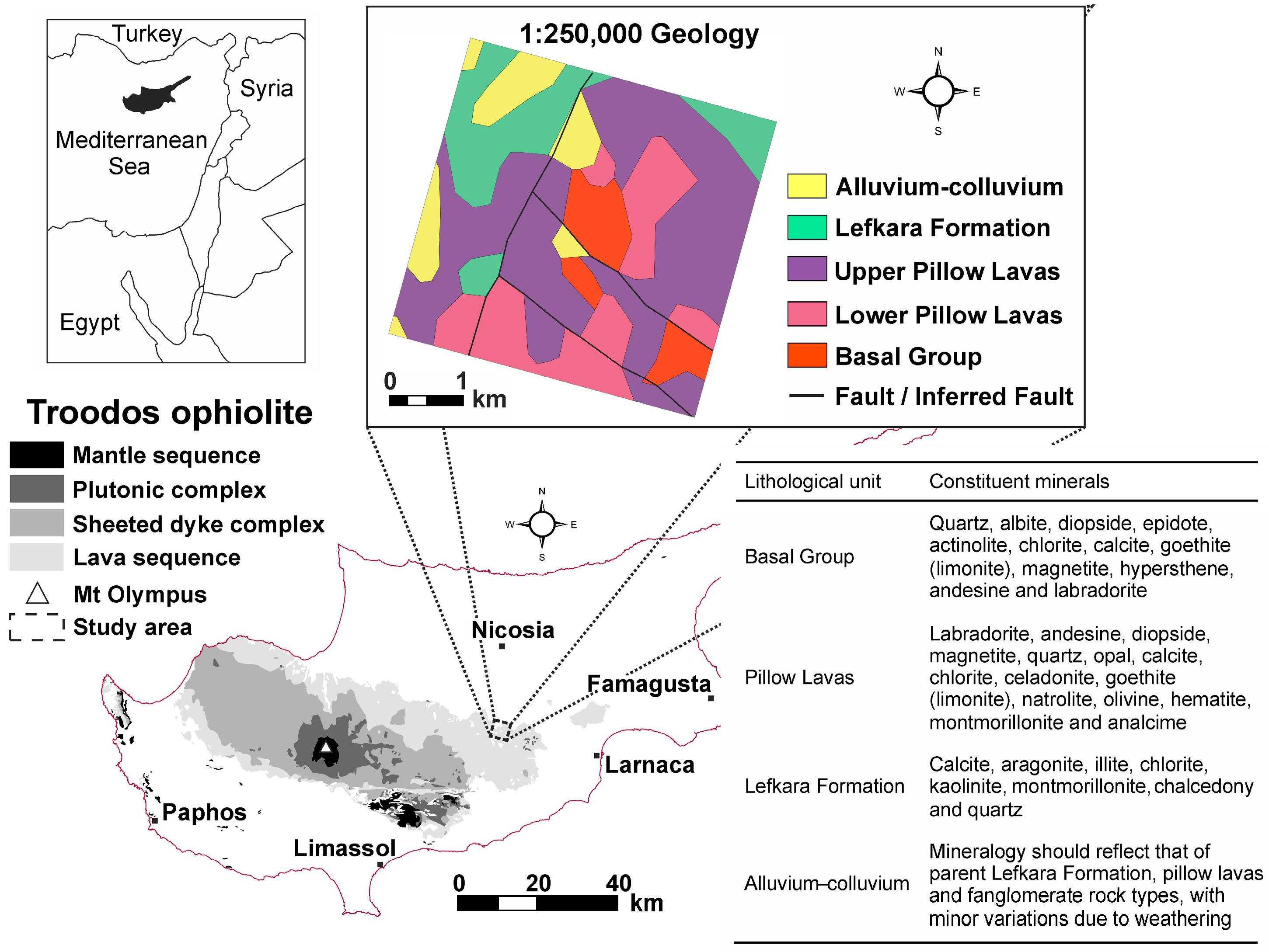
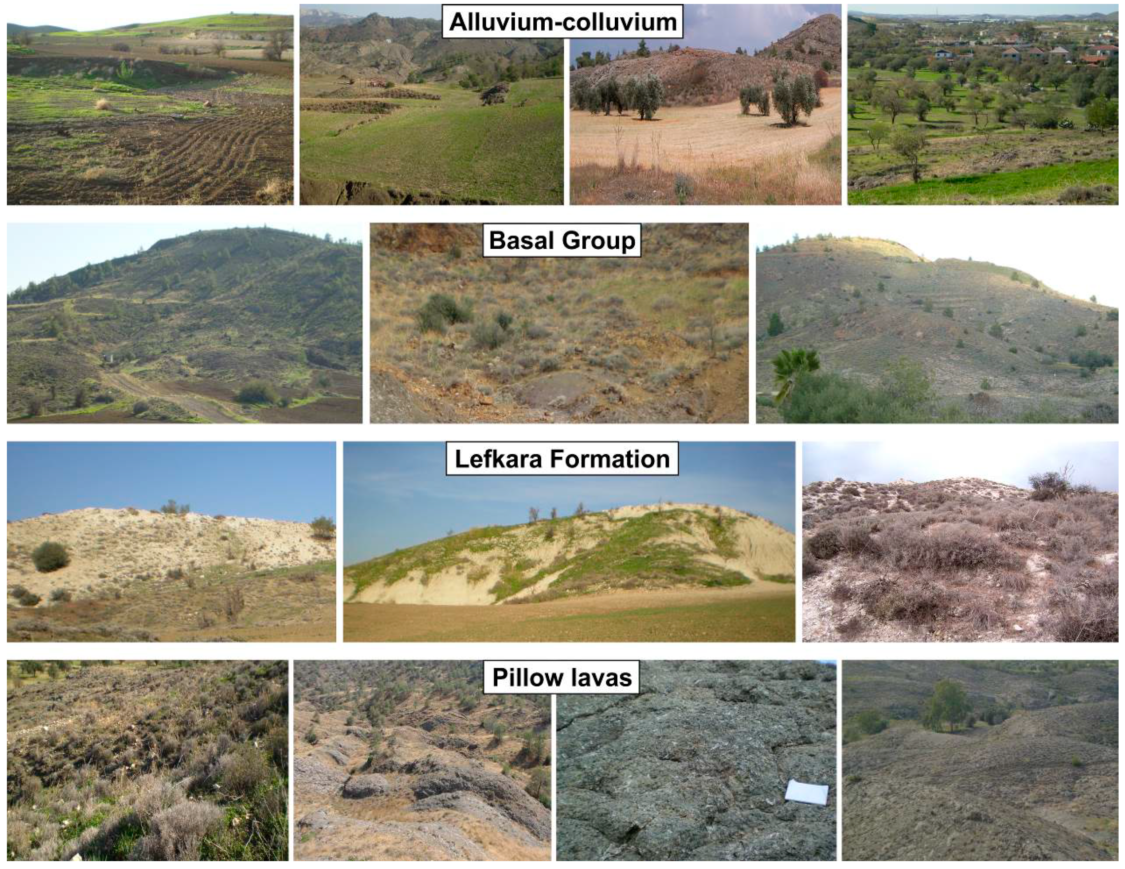
2. Study Area
3. Methods
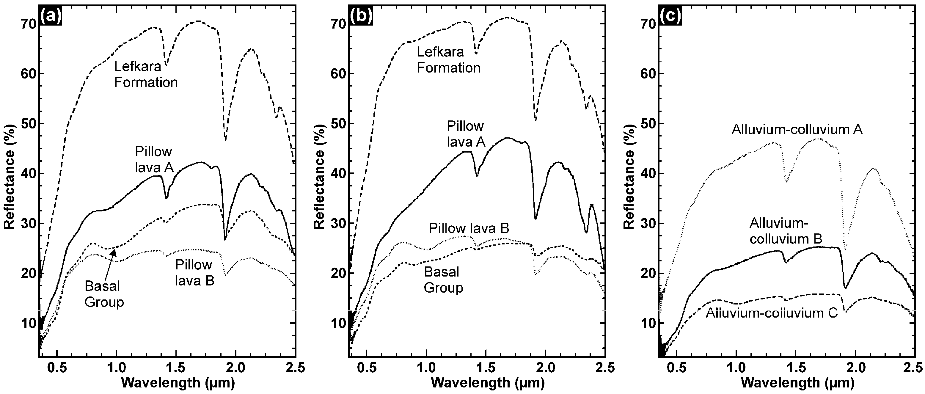
3.1. Spectral Signatures of the Lithological Units
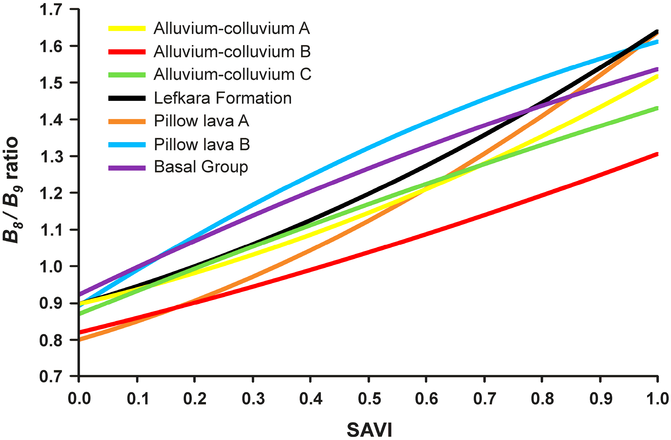
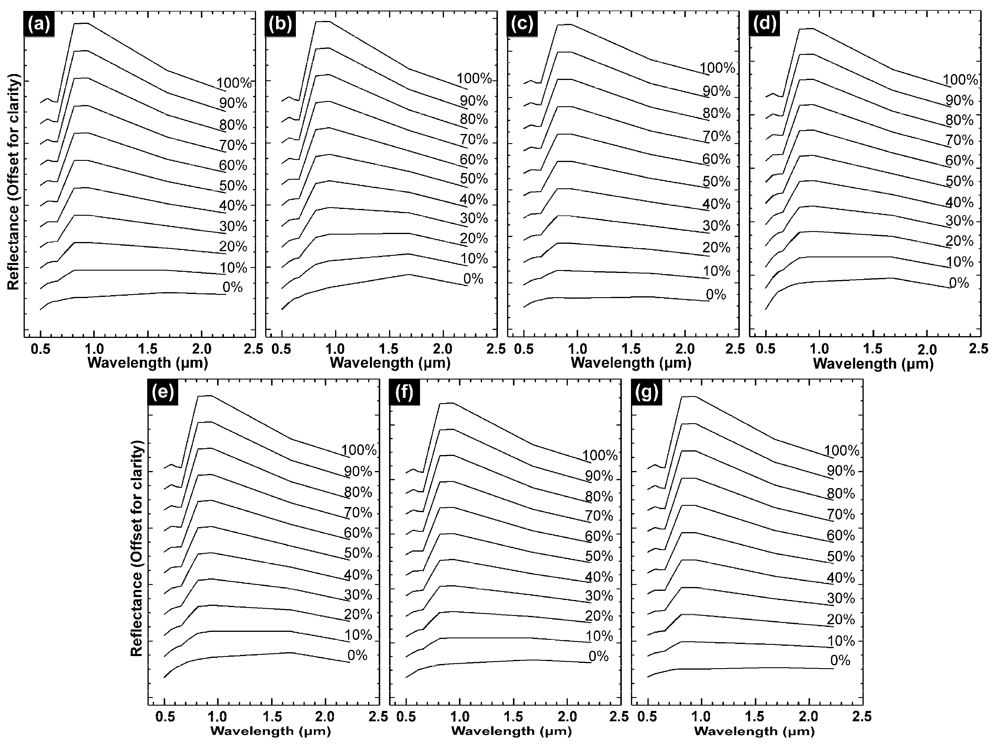
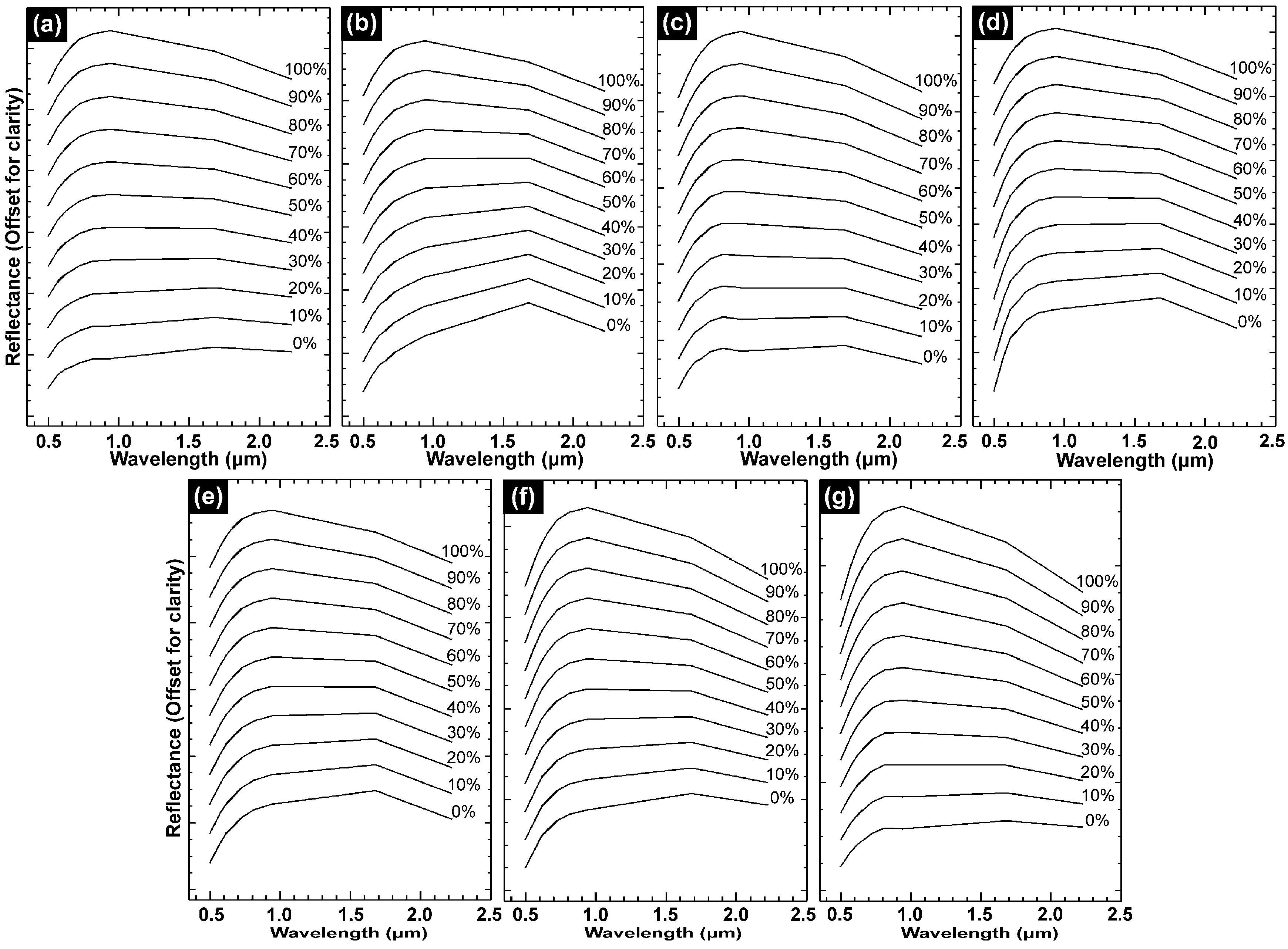
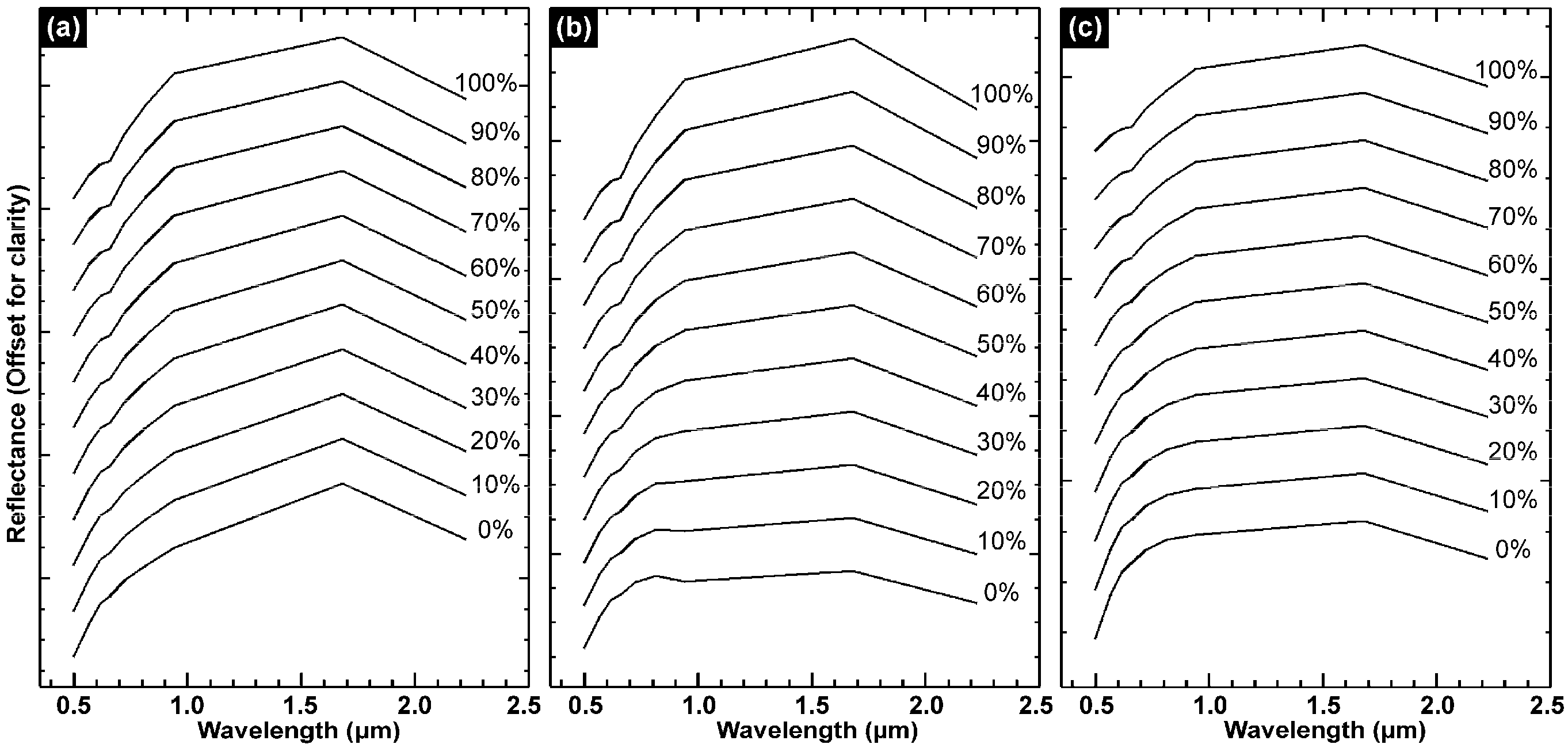
3.2. Modeling the Impact of Vegetation on the Spectra of the Four Lithologies
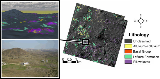
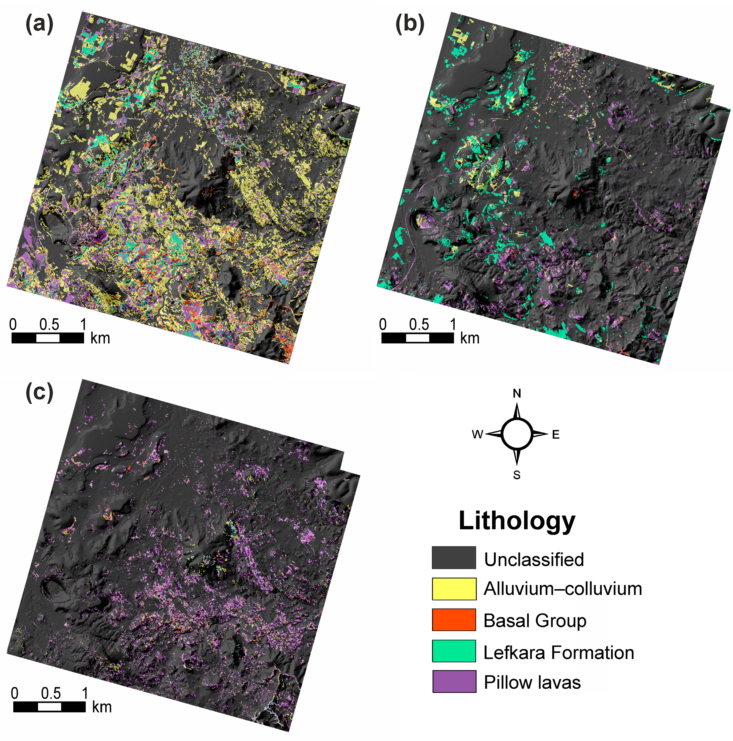
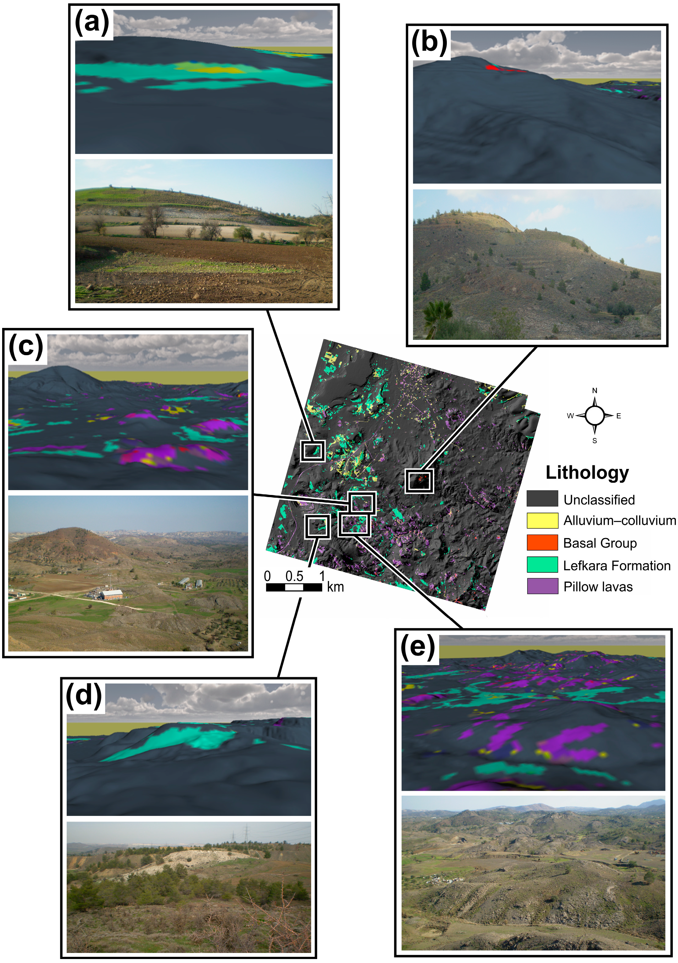
3.3. Remote Lithological Mapping and the Impact of Vegetation
3.3.1. Airborne Multispectral Imagery

| ATM Band | Wavelength (μm) | Spectral Region | Equivalent Landsat 8 Band | Equivalent Sentinel-2 Band | Equivalent WorldView-3 Band |
|---|---|---|---|---|---|
| 1 | 0.42–0.45 | Ultraviolet/blue | 1 | 1 | Coastal |
| 2 | 0.45–0.52 | Blue | 2 | 2 | Blue |
| 3 | 0.52–0.60 | Green | 3 | 3 | Green |
| 4 | 0.60–0.62 | Yellow/orange | Yellow | ||
| 5 | 0.63–0.69 | Red | 4 | 4 | Red |
| 6 | 0.69–0.75 | Near-infrared | 5 and 6 | Red Edge | |
| 7 | 0.76–0.90 | Near-infrared | 5 | 7, 8, 8a | Near-IR1 |
| 8 | 0.91–1.05 | Near-infrared | 9 | Near-IR2 | |
| 9 | 1.55–1.75 | Shortwave infrared | 6 | 11 | SWIR-2,3,4 |
| 10 | 2.08–2.35 | Shortwave infrared | 7 | 12 | SWIR-5,6,7,8 |
| 11 | 8.50–13.00 | Thermal infrared | 10 and 11 |
3.3.2. Data Calibration
3.3.3. Image Classification
3.3.4. Classification Performance
3.3.5. Vegetation Abundance
4. Results and Discussion
4.1. Spectral Signatures of the Lithological Units
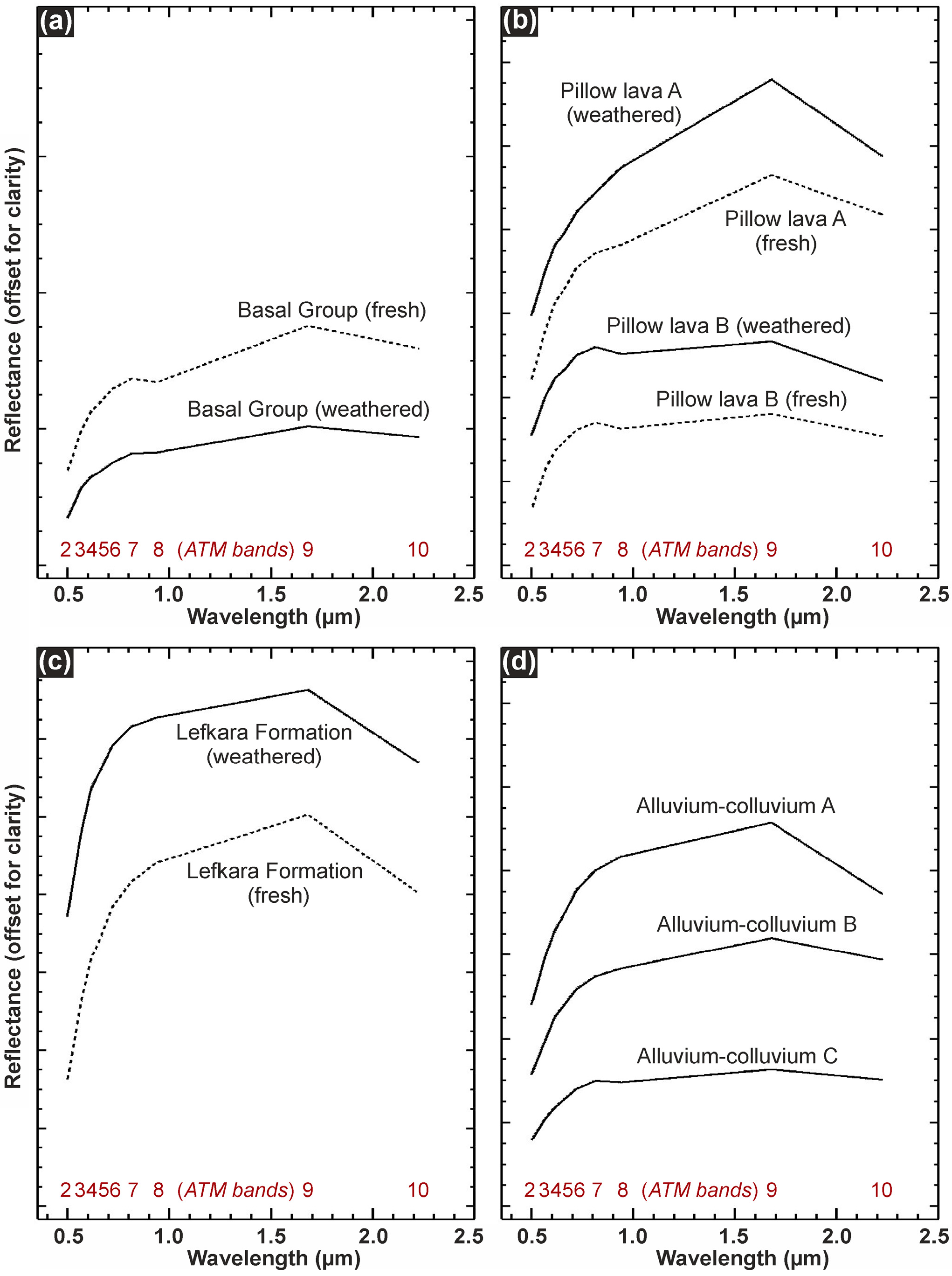
4.2. Impact of Vegetation on Spectral Recognition of the Lithologies
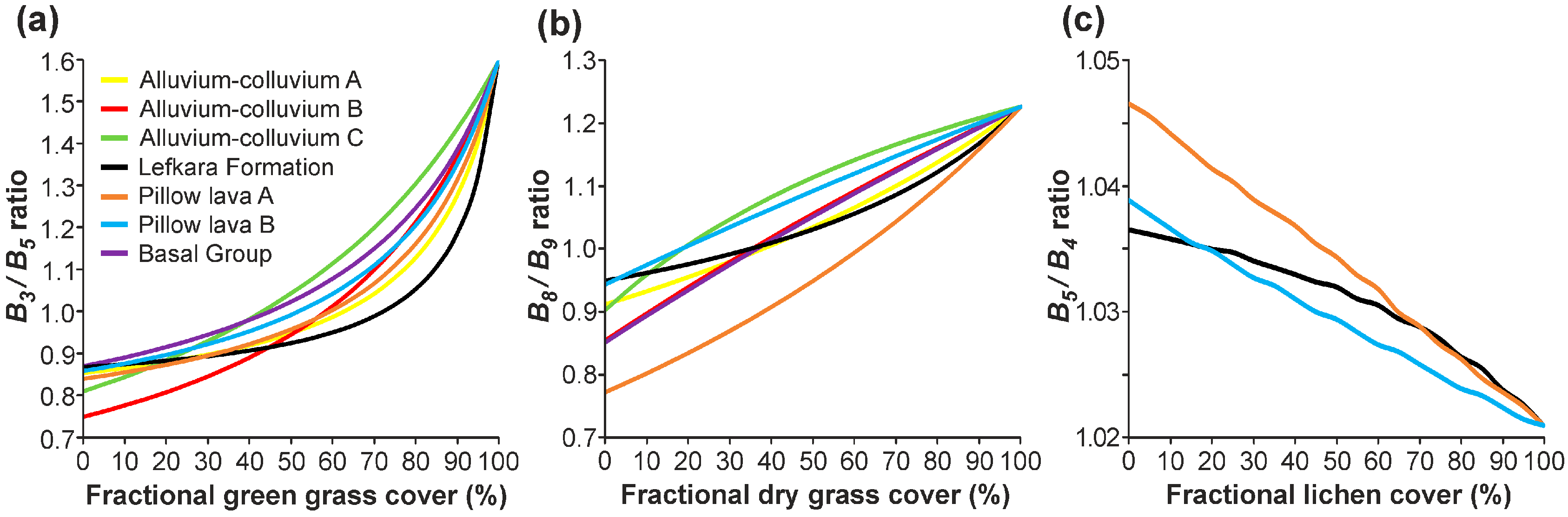
4.3. Implications for Spectral Recognition Using Airborne Multispectral Imagery

4.4. Impact of Vegetation on Remote Lithological Mapping

| SAM | Validation Data | Row Total | UA (%) | ||||
| Mapped as | AC | BG | LF | PL | |||
| Unclassified | 3299 | 2544 | 1969 | 1875 | 9687 | - | |
| AC | 589 | 542 | 393 | 1046 | 2570 | 22.9 | |
| BG | 1 | 61 | 12 | 93 | 167 | 36.5 | |
| LF | 34 | 2 | 50 | 52 | 138 | 36.2 | |
| PL | 164 | 51 | 27 | 142 | 384 | 37.0 | |
| Column total | 4087 | 3200 | 2451 | 3208 | |||
| PA (%) | 14.4 | 1.9 | 2.0 | 4.4 | |||
| Overall accuracy = 6.5% | |||||||
| K = −0.01 | |||||||
| MF | Validation Data | Row Total | UA (%) | ||||
| Mapped as | AC | BG | LF | PL | |||
| Unclassified | 4006 | 3052 | 2315 | 2960 | 12333 | - | |
| AC | 31 | 0 | 65 | 21 | 117 | 26.5 | |
| BG | 0 | 0 | 0 | 17 | 17 | 0.0 | |
| LF | 50 | 84 | 67 | 0 | 201 | 33.3 | |
| PL | 0 | 64 | 4 | 210 | 278 | 75.5 | |
| Column total | 4087 | 3200 | 2451 | 3208 | |||
| PA (%) | 0.8 | 0.0 | 2.7 | 6.5 | |||
| Overall accuracy = 2.4% | |||||||
| K = 0.01 | |||||||
| SFF | Validation Data | Row Total | UA (%) | ||||
| Mapped as | AC | BG | LF | PL | |||
| Unclassified | 3964 | 3947 | 2445 | 2690 | 12046 | - | |
| AC | 10 | 65 | 0 | 79 | 154 | 6.5 | |
| BG | 1 | 1 | 0 | 1 | 3 | 33.3 | |
| LF | 16 | 49 | 3 | 100 | 168 | 1.8 | |
| PL | 96 | 138 | 3 | 338 | 575 | 58.8 | |
| Column total | 4087 | 3200 | 2451 | 3208 | |||
| PA (%) | 0.2 | 0.0 | 0.1 | 10.5 | |||
| Overall accuracy = 2.7% | |||||||
| K = 0.01 | |||||||
| Classified | Unclassified | p-value | ||||||||
|---|---|---|---|---|---|---|---|---|---|---|
| Classifier | n | Mean | SD | n | Mean | SD | ||||
| Validation pixels | SAM | 3259 | 0.30 | 0.13 | 9687 | 0.67 | 0.19 | <0.0001 | ||
| MF | 613 | 0.23 | 0.15 | 12,333 | 0.59 | 0.23 | <0.0001 | |||
| SFF | 900 | 0.29 | 0.11 | 12,046 | 0.60 | 0.23 | <0.0001 | |||
| All scene pixels | SAM | 259,230 | 0.27 | 0.13 | 498,570 | 0.63 | 0.22 | <0.0001 | ||
| MF | 78,089 | 0.20 | 0.18 | 679,711 | 0.54 | 0.24 | <0.0001 | |||
| SFF | 57,279 | 0.26 | 0.11 | 700,521 | 0.53 | 0.26 | <0.0001 | |||

5. Conclusions
Acknowledgments
Author Contributions
Conflicts of Interest
References
- Hunt, G.R. Spectral signatures of particulate minerals in visible and near infrared. Geophysics 1977, 42, 501–513. [Google Scholar] [CrossRef]
- Rothery, D.A. Improved discrimination of rock units using Landsat Thematic Mapper imagery of the Oman ophiolite. J. Geol. Soc. 1987, 144, 587–597. [Google Scholar] [CrossRef]
- van der Meer, F.D.; van der Werff, H.M.A.; van Ruitenbeek, F.J.A.; Hecker, C.A.; Bakker, W.H.; Noomen, M.F.; van der Meijde, M.; Carranza, E.J.M.; de Smeth, J.B.; Woldai, T. Multi- and hyperspectral geologic remote sensing: A review. Int. J. Appl. Earth Obs. Geoinf. 2012, 14, 112–128. [Google Scholar]
- Hunt, G.R.; Salisbury, J.W. Visible and near infrared spectra of minerals and rocks: I Silicate minerals. Mod. Geol. 1970, 1, 283–300. [Google Scholar]
- Hunt, G.R.; Salisbury, J.W. Visible and near infrared spectra of minerals and rocks: II Carbonates. Mod. Geol. 1971, 2, 23–30. [Google Scholar]
- Hunt, G.R.; Salisbury, J.W.; Lenhoff, J.C. Visible and near-infrared spectra of minerals and rocks: IV Sulphides and sulphates. Mod. Geol. 1971, 3, 1–14. [Google Scholar]
- Hunt, G.R.; Salisbury, J.W.; Lenhoff, J.C. Visible and near-infrared spectra of minerals and rocks: V Halides, phosphates, arsenates, vanadates and borates. Mod. Geol. 1972, 3, 121–132. [Google Scholar]
- Adams, J.B. Visible and near-infrared diffuse reflectance spectra of pyroxenes as applied to remote-sensing of solid objects in solar-system. J. Geophys. Res. 1974, 79, 4829–4836. [Google Scholar] [CrossRef]
- Clark, R.N.; King, T.V.V.; Klejwa, M.; Swayze, G.A.; Vergo, N. High spectral resolution reflectance spectroscopy of minerals. J. Geophys. Res. 1990, 95, 12653–12680. [Google Scholar] [CrossRef]
- van der Meer, F.; Vazquez-Torres, M.; van Dijk, P.M. Spectral characterization of ophiolite lithologies in the Troodos Ophiolite complex of Cyprus and its potential in prospecting for massive sulphide deposits. Int. J. Remote Sens. 1997, 18, 1245–1257. [Google Scholar] [CrossRef]
- Rowan, L.C.; Mars, J.C. Lithologic mapping in the Mountain Pass, California area using advanced Spaceborne thermal emission and reflection radiometer (ASTER) data. Remote Sens. Environ. 2003, 84, 350–366. [Google Scholar] [CrossRef]
- Rowan, L.C.; Simpson, C.J.; Mars, J.C. Hyperspectral analysis of the ultramafic complex and adjacent lithologies at Mordor, NT, Australia. Remote Sens. Environ. 2004, 91, 419–431. [Google Scholar] [CrossRef]
- Rowan, L.C.; Mars, J.C.; Simpson, C.J. Lithologic mapping of the Mordor, NT, Australia ultramafic complex by using the Advanced Spaceborne Thermal emission and Reflection Radiometer (ASTER). Remote Sens. Environ. 2005, 99, 105–126. [Google Scholar] [CrossRef]
- Harris, J.R.; Rogge, D.; Hitchcock, R.; Ijewliw, O.; Wright, D. Mapping lithology in Canada’s Arctic: Application of hyperspectral data using the minimum noise fraction transformation and matched filtering. Can. J. Earth Sci. 2005, 42, 2173–2193. [Google Scholar] [CrossRef]
- Bedini, E. Mapping lithology of the Sarfartoq carbonatite complex, southern West Greenland, using HyMap imaging spectrometer data. Remote Sens. Environ. 2009, 113, 1208–1219. [Google Scholar] [CrossRef]
- Roy, R.; Launeau, P.; Carrere, V.; Pinet, P.; Ceuleneer, G.; Clenet, H.; Daydou, Y.; Girardeau, J.; Amri, I. Geological mapping strategy using visible near-infrared-shortwave infrared hyperspectral remote sensing: Application to the Oman ophiolite (Sumail Massif). Geochem. Geophy. Geosy. 2009, 10. [Google Scholar] [CrossRef]
- Haselwimmer, C.E.; Riley, T.R.; Liu, J.G. Assessing the potential of multispectral remote sensing for lithological mapping on the Antarctic Peninsula: Case study from eastern Adelaide Island, Graham Land. Antarct. Sci. 2010, 22, 299–318. [Google Scholar] [CrossRef]
- Tangestani, M.H.; Jaffari, L.; Vincent, R.K.; Sridhar, B.B.M. Spectral characterization and ASTER-based lithological mapping of an ophiolite complex: A case study from Neyriz ophiolite, SW Iran. Remote Sens. Environ. 2011, 115, 2243–2254. [Google Scholar] [CrossRef]
- van der Meer, F.D.; van der Werff, H.M.A.; van Ruitenbeek, F.J.A. Potential of ESA’s Sentinel-2 for geological applications. Remote Sens. Environ. 2014, 148, 124–133. [Google Scholar] [CrossRef]
- Fraser, S.J.; Green, A.A. A software defoliant for geological analysis of band ratios. Int. J. Remote Sens. 1987, 8, 525–532. [Google Scholar] [CrossRef]
- Carranza, E.J.M.; Hale, M. Mineral imaging with Landsat Thematic Mapper data for hydrothermal alteration mapping in heavily vegetated terrane. Int. J. Remote Sens. 2002, 23, 4827–4852. [Google Scholar] [CrossRef]
- Siegal, B.S.; Goetz, A.F.H. Effect of vegetation on rock and soil type discrimination. Photogramm. Eng. Remote Sens. 1977, 43, 191–196. [Google Scholar]
- Murphy, R.J.; Wadge, G. The effects of vegetation on the ability to map soils using imaging spectrometer data. Int. J. Remote Sens. 1994, 15, 63–86. [Google Scholar] [CrossRef]
- Ager, C.M.; Milton, N.M. Spectral reflectance of lichens and their effects on the reflectance of rock substrates. Geophysics 1987, 52, 898–906. [Google Scholar] [CrossRef]
- Crippen, R.E.; Blom, R.G. Unveiling the lithology of vegetated terrains in remotely sensed imagery. Photogramm. Eng. Remote Sens. 2001, 67, 935–943. [Google Scholar]
- Bierwirth, P.N. Mineral mapping and vegetation removal via data-calibrated pixel unmixing, using multispectral. Int. J. Remote Sens. 2009, 11, 1999–1207. [Google Scholar] [CrossRef]
- Chabrillat, S.; Pinet, P.C.; Ceuleneer, G.; Johnson, P.E.; Mustard, J.F. Ronda peridotite massif: Methodology for its geological mapping and lithological discrimination from airborne hyperspectral data. Int. J. Remote Sens. 2000, 21, 2363–2388. [Google Scholar] [CrossRef]
- Asner, G.P.; Heidebrecht, K.B. Spectral unmixing of vegetation, soil and dry carbon cover in arid regions: Comparing multispectral and hyperspectral observations. Int. J. Remote Sens. 2002, 23, 3939–3958. [Google Scholar] [CrossRef]
- Zhang, J.; Rivard, B.; Sanchez-Azofeifa, A. Spectral unmixing of normalized reflectance data for the deconvolution of lichen and rock mixtures. Remote Sens. Environ. 2005, 95, 57–66. [Google Scholar] [CrossRef]
- Morison, M.; Cloutis, E.; Mann, P. Spectral unmixing of multiple lichen species and underlying substate. Int. J. Remote Sens. 2014, 35, 478–492. [Google Scholar] [CrossRef]
- Rogge, D.; Rivard, B.; Segl, K.; Grant, B.; Feng, J. Mapping of NiCu–PGE ore hosting ultramafic rocks using airborne and simulated EnMAP hyperspectral imagery, Nunavik, Canada. Remote Sens. Environ. 2014, 152, 302–317. [Google Scholar] [CrossRef]
- Schetselaar, E.M.; Chung, C.J.F.; Kim, K.E. Integration of Landsat TM, gamma-ray, magnetic, and field data to discriminate lithological units in vegetated granite-gneiss terrain. Remote Sens. Environ. 2000, 71, 89–105. [Google Scholar] [CrossRef]
- Dong, P.; Leblon, B. Rock unit discrimination on Landsat TM, SIR-C and Radarsat images using spectral and textural information. Int. J. Remote Sens. 2004, 25, 3745–3768. [Google Scholar] [CrossRef]
- Grebby, S.; Naden, J.; Cunningham, D.; Tansey, K. Integrating airborne multispectral imagery and airborne LiDAR data for enhanced lithological mapping in vegetated terrain. Remote Sens. Environ. 2011, 115, 214–226. [Google Scholar] [CrossRef]
- Rodger, A.; Cudahy, T. Vegetation corrected continuum depths at 2.20 µm: An approach for hyperspectral sensors. Remote Sens. Environ. 2009, 113, 2243–2257. [Google Scholar] [CrossRef]
- Haest, M.; Cudahy, T.; Rodger, A.; Laukamp, C.; Martens, E.; Caccetta, M. Unmixing the effects of vegetation in airborne hyperspectral mineral maps over the Rocklea Dome iron-rich palaeochannel system (Western Australia). Remote Sens. Environ. 2013, 129, 17–31. [Google Scholar] [CrossRef]
- Satterwhite, M.B.; Henley, J.P.; Carney, J.M. Effects of lichens on the reflectance spectra of granitic rock surfaces. Remote Sens. Environ. 1985, 18, 105–112. [Google Scholar] [CrossRef]
- Rivard, B.; Arvidson, R.E. Utility of imaging spectrometry for lithologic mapping in Greenland. Photogramm. Eng. Remote Sens. 1992, 58, 945–949. [Google Scholar]
- Feng, J.; Rivard, B.; Rogge, D.; Sanchez-Azofeifa, A. The longwave infrared (3–14 μm) spectral properties of rock encrusting lichens based on laboratory spectra and airborne SEBASS imagery. Remote Sens. Environ. 2013, 131, 173–181. [Google Scholar] [CrossRef]
- Gass, I.G. Is the troodos massif of Cyprus a fragment of mesozoic ocean crust? Nat. 1968, 220, 39–42. [Google Scholar]
- Moores, E.M.; Vine, F.J. Troodos Massif, Cyprus and other ophiolites as oceanic crust: Evaluation and implications. Philos. T. R. Soc. A 1971, 268, 443–467. [Google Scholar] [CrossRef]
- Varga, R.J.; Moores, E.M. Spreading structure of the Troodos ophiolite, Cyprus. Geology 1985, 13, 846–850. [Google Scholar] [CrossRef]
- Gass, I.G. The Geology and Mineral Resources of the Dhali Area; Geological Survey Department: Lefkosia, Cyprus, 1960. [Google Scholar]
- Grebby, S.; Cunningham, D.; Naden, J.; Tansey, K. Lithological mapping of the Troodos ophiolite, Cyprus, using airborne LiDAR topographic data. Remote Sens. Environ. 2010, 114, 713–724. [Google Scholar]
- Grebby, S.; Cunningham, D.; Naden, J.; Tansey, K. Application of airborne LiDAR data and airborne multispectral imagery to structural mapping of the upper section of the Troodos ophiolite, Cyprus. Int. J. Earth Sci. 2012, 101, 1645–1660. [Google Scholar] [CrossRef]
- Kruse, F.A.; Lefkoff, A.B.; Boardman, J.W.; Heidebrecht, K.B.; Shapiro, A.T.; Barloon, P.J.; Goetz, A.F.H. The Spectral Image-Processing System (SIPS)—Interactive visualization and analysis of imaging spectrometer data. Remote Sens. Environ. 1993, 44, 145–163. [Google Scholar] [CrossRef]
- Singer, R.B.M.; McCord, T.B. Mars: Large scale mixing of bright and dark surface materials and implications for analysis of spectral reflectance. In Proceedings of the 10th Lunar and Planetary Science Conference, Houston, TX, USA, 19–23 March 1979; Pergamon Press, Inc.: New York, NY, USA; pp. 1835–1848.
- Roberts, D.A.; Yamaguchi, Y.; Lyon, R.J.P. Calibration of airborne imaging spectrometer data to percent reflectance using field spectral measurements. In Proceedings of 19th International Symposium on Remote Sensing of Environment, Ann Arbor, MI, USA, 21 October 1985; pp. 679–688.
- Baugh, W.M.; Groeneveld, D.P. Empirical proof of the empirical line. Int. J. Remote Sens. 2008, 29, 665–672. [Google Scholar] [CrossRef]
- Ferrier, G. Evaluation of apparent surface reflectance estimation methodologies. Int. J. Remote Sens. 1995, 16, 2291–2297. [Google Scholar] [CrossRef]
- van der Meer, F.; Bakker, W. Cross correlogram spectral matching: application to surface mineralogical mapping by using AVIRIS data from Cuprite, Nevada. Remote Sens. Environ. 1997, 61, 371–382. [Google Scholar] [CrossRef]
- Price, J.C.; Anger, C.D.; Mah, S. Preliminary evaluation of casi preprocessing techniques. In Proceedings of the 17th Canadian Symposium on Remote Sensing, Saskatoon, SK, Canada, 13–15 June 1995; Canadian Remote Sensing Society and Canadian Aeronautics and Space Institute: Ontario, ON, Canada; pp. 649–697.
- Smith, G.M.; Milton, E.J. The use of the empirical line method to calibrate remotely sensed data to reflectance. Int. J. Remote Sens. 1999, 20, 2653–2662. [Google Scholar] [CrossRef]
- Harsanyi, J.C.; Chang, C.I. Hyperspectral image classification and dimensionality reduction—An orthogonal subspace projection approach. IEEE Trans. Geosci. Remote Sens. 1994, 32, 779–785. [Google Scholar] [CrossRef]
- Green, A.A.; Berman, M.; Switzer, P.; Craig, M.D. A transformation for ordering multispectral data in terms of image quality with implications for noise removal. IEEE Trans. Geosci. Remote Sens. 1988, 26, 65–74. [Google Scholar]
- Mundt, J.; Streutker, D.; Glenn, N. Prtial unmixing of hyperspectral imagery: Theory and methods. In Proceedings of the American Society for Photogrammetry and Remote Sensing, Tampa, FL, USA, 7–11 May 2007.
- Mitchell, J.J.; Glenn, N.F. Subpixel abundance estimates in mixture-tuned matched filtering classifications of leafy spurge (Euphorbia esula L.). Int. J. Remote Sens. 2009, 30, 6099–6119. [Google Scholar] [CrossRef]
- Clark, R.N.; Gallagher, A.J.; Swayze, G.A. Material absorption band depth mapping of imaging spectrometer data using the complete band shape least squares algorithm simultaneously fit to multiple spectral features from multiple materials. In Proceedings of the Second Airborne Visible/Infrared Imaging Spectrometer (AVIRIS) Workshop, Pasadena, CA, USA, 4–5 June 1990; pp. 176–186.
- Clark, R.N.; Swayze, G.A.; Gallagher, A.; Gorelick, N.; Kruse, F.A. Mapping with imaging spectrometer data using the complete band shape least-squares algorithm simultaneously fit to multiple spectral features from multiple materials. In Proceedings of the Third Airborne Visible/Infrared Imaging Spectrometer (AVIRIS) Workshop, Pasadena, CA, USA, 20–21 May 1991; pp. 2–3.
- Clark, R.N.; Swayze, G.A.; Gallagher, A. Mapping the mineralogy and lithology of Canyonlands, Utah with imaging spectrometer data and the multiple spectral feature mapping algorithm. In Proceedings of the Third Annual JPL Airborne Geoscience Workshop, Pasadena, CA, USA, 1–5 June 1992; pp. 11–13.
- Clark, R.N.; Roush, T.L. Reflectance spectroscopy—Quantitative analysis techniques for remote-sensing applications. J. Geophys. Res. 1984, 89, 6329–6340. [Google Scholar] [CrossRef]
- Clark, R.N.; Swayze, G.A.; Livo, K.E.; Kokaly, R.F.; Sutley, S.J.; Dalton, J.B.; McDougal, R.R.; Gent, C.A. Imaging spectroscopy: Earth and planetary remote sensing with the USGS Tetracorder and expert systems. J. Geophys. Res. Planet. 2003, 108. [Google Scholar] [CrossRef]
- Crowley, J.K.; Williams, D.E.; Hammarstrom, J.M.; Piatak, N.; Chou, I-M.; Mars, J.C. Spectral reflectance properties (0.4–2.5 μm) of secondary Fe-oxide, Fe-hydroxide, and Fe-sulphate-hydrate minerals associated with sulphide-bearing mine wastes. Geochem. Explor. Environ. Anal. 2003, 3, 219–228. [Google Scholar] [CrossRef]
- Congalton, R.G. A review of assessing the accuracy of classifications of remotely sensed data. Remote Sens. Environ. 1991, 37, 35–46. [Google Scholar] [CrossRef]
- Chini, M.; Pacifici, F.; Emery, W.J.; Pierdicca, N.; Del Frate, F. Comparing statistical and neural network methods applied to very high resolution satellite images showing changes in man-made structures at rocky flats. IEEE Trans. Geosci. Remote Sens. 2008, 46, 1812–1821. [Google Scholar] [CrossRef]
- Pacifici, F.; Chini, M.; Emery, W.J. A neural network approach using multi-scale textural metrics from very high-resolution panchromatic imagery for urban land-use classification. Remote Sens. Environ. 2009, 113, 1276–1292. [Google Scholar]
- Huete, A.R. A soil-adjusted vegetation index (SAVI). Remote Sens. Environ. 1988, 25, 295–309. [Google Scholar] [CrossRef]
- Leprieur, C.; Verstraete, M.M.; Pinty, B. Evaluation of the performance of various vegetation indices to retrieve vegetation cover from AVHRR data. Remote Sens. Rev. 1994, 10, 265–284. [Google Scholar] [CrossRef]
- Huete, A.R.; Liu, H.Q.; Batchily, K.; van Leeuwen, W. A comparison of vegetation indices over a global set of TM images for EOS-MODIS. Remote Sens. Environ. 1997, 59, 440–451. [Google Scholar] [CrossRef]
- Vincent, R.K.; Hunt, G.R. Infrared reflectance from mat surfaces. Appl. Opt. 1968, 7, 53–59. [Google Scholar]
- Constantinou, G. The Geology and Genesis of The Sulphide Ores of Cyprus. PhD Thesis, University of London, London, UK, 1972. [Google Scholar]
- Marsh, S.E.; McKeon, J.B. Integrated analysis of high-resolution field and airborne spectroradiometer data for alteration mapping. Econ. Geol. 1983, 78, 618–632. [Google Scholar] [CrossRef]
- Morris, R.V.; Lauer, H.V.; Lawson, C.A.; Gibson, E.K.; Nace, G.A.; Stewart, C. Spectral and other physicochemical properties of submicron powders of hematite (Alpha-Fe2O3), maghemite (Gamma-Fe2O3), magnetite (Fe3O4), goethite (Alpha-Feooh), and lepidocrocite (Gamma-Feooh). J. Geophys. Res. 1985, 90, 3126–3144. [Google Scholar] [CrossRef] [PubMed]
- Bear, L.M. The Geology and Mineral Resources of the Akaki.-Lythrodondha Area; Geological Survey Department: Lefkosia, Cyprus, 1960. [Google Scholar]
- Bishop, J.L.; Lane, M.D.; Dyar, M.D.; Brown, A.J. Reflectance and emission spectroscopy study of four groups of phyllosilicates: Smectites, kaolinite-serpentines, chlorites and micas. Clay Miner. 2008, 43, 35–54. [Google Scholar] [CrossRef]
- Rosenfield, G.H.; Fitzpatrick-Lins, K. A coefficient of agreement as a measure of thematic classification accuracy. Photogramm. Eng. Remote Sens. 1986, 52, 223–227. [Google Scholar]
- Murphy, R.J.; Monteiro, S.T.; Schneider, S. Evaluating classification techniques for mapping vertical geology using field-based hyperspectral sensors. IEEE Trans. Geosci. Remote Sens. 2012, 50, 3066–3080. [Google Scholar]
- Leverington, D.W. Discrimination of sedimentary lithologies using Hyperion and Landsat Thematic Mapper data: A case study at Melville Island, Canadian High Arctic. Int. J. Remote Sens. 2010, 31, 233–260. [Google Scholar] [CrossRef]
© 2014 by the authors; licensee MDPI, Basel, Switzerland. This article is an open access article distributed under the terms and conditions of the Creative Commons Attribution license (http://creativecommons.org/licenses/by/4.0/).
Share and Cite
Grebby, S.; Cunningham, D.; Tansey, K.; Naden, J. The Impact of Vegetation on Lithological Mapping Using Airborne Multispectral Data: A Case Study for the North Troodos Region, Cyprus. Remote Sens. 2014, 6, 10860-10887. https://doi.org/10.3390/rs61110860
Grebby S, Cunningham D, Tansey K, Naden J. The Impact of Vegetation on Lithological Mapping Using Airborne Multispectral Data: A Case Study for the North Troodos Region, Cyprus. Remote Sensing. 2014; 6(11):10860-10887. https://doi.org/10.3390/rs61110860
Chicago/Turabian StyleGrebby, Stephen, Dickson Cunningham, Kevin Tansey, and Jonathan Naden. 2014. "The Impact of Vegetation on Lithological Mapping Using Airborne Multispectral Data: A Case Study for the North Troodos Region, Cyprus" Remote Sensing 6, no. 11: 10860-10887. https://doi.org/10.3390/rs61110860
APA StyleGrebby, S., Cunningham, D., Tansey, K., & Naden, J. (2014). The Impact of Vegetation on Lithological Mapping Using Airborne Multispectral Data: A Case Study for the North Troodos Region, Cyprus. Remote Sensing, 6(11), 10860-10887. https://doi.org/10.3390/rs61110860