Abstract
We report on the development and characterization of the new compact infrared heterodyne receiver, iChips (Infrared Compact Heterodyne Instrument for Planetary Science). It is specially designed for ground-based observations of the terrestrial atmosphere in the mid-infrared wavelength region. Mid-infrared room temperature quantum cascade lasers are implemented into a heterodyne system for the first time. Their tunability allows the instrument to operate in two different modes. The scanning mode covers a spectral range of few wavenumbers continuously with a resolution of approximately
. This mode allows the determination of the terrestrial atmospheric transmission. The staring mode, applied for observations of single molecular transition features, provides a spectral resolution of
and a bandwidth of 1.4 GHz. To demonstrate the instrument’s capabilities, initial observations in both modes were performed by measuring the terrestrial transmittance at 7.8 μm (∼ 1,285 cm−1) and by probing terrestrial ozone features at 8.6 μm (∼ 1,160 cm−1), respectively. The receivers characteristics and performance are described.
Keywords:
heterodyne; infrared; spectroscopy; atmosphere; transmission; ultra-high resolution; ozone; trace gas; wind 1. Introduction
Heterodyne spectroscopy is a powerful tool to observe the atmospheres of terrestrial planets. It provides ultra high spectral resolution of
, yielding the capability to resolve single molecular transition features [1]. Fully resolved molecular transitions provide information about physical parameters, like temperatures, abundances or dynamical properties. In recent years, this technique has been established to derive ground-based direct wind and temperature measurements by remote sensing of Doppler-shifted and -broadened molecular transitions in the mid-infrared (mid-IR) wavelength regime. Detailed investigations on the dynamical and thermal properties of the upper atmospheres of Titan [2,3], Venus [4–6] and Mars [7] have been accomplished. Furthermore, observations of the molecular abundances of Martian ozone were conducted [8].
High resolution spectroscopy can also be deployed on Earth’s atmosphere. One interesting topic is the tracking of the dynamical behavior in the Earth atmosphere. Hence, investigations to obtain a comprehensive picture are enormous. Ground-based IR heterodyne observations could support ongoing efforts. Analysis of Doppler shifted molecular features is a common technique to observe terrestrial atmospheric dynamics. It is conducted by several airborne and spaceborne instruments, i.e., the High Resolution Doppler Imager on the Upper Atmosphere Research Satellite, determining winds in an altitude region between 10 km and 40 km [9], the sub-millimeter limb-sounder Smiles on board the International Space Station (35–60 km) [10], the ADM-Aeolus (Atmospheric Dynamics Mission) ESA satellite mission (launch 2013) with its Doppler LiDAR instrument Aladin [11], which operates at the UV wavelength and probes an altitude region between 26 km and the ground, and the Swift mission [12], designed to observe ozone emission features in the mid-infrared. Airborne platforms can provide very high vertical resolution and precision, but they possess spatial limits, due to their orbits.
Recently, ground-based observation by remote sensing with two combined LiDAR instruments between 30 km and 110 km [13] were conducted. Furthermore, ground-based observations of vertical wind profiles, using a microwave Doppler spectroradiometer [14], have been performed by probing ozone emission features, originating from an altitude region between 30 km and 70 km.
An additional challenge in observing terrestrial trace gases is the investigation of methane abundances. Methane plays a significant role in the terrestrial greenhouse effect, and its anthropogenic sources are unquestioned. Its sinks, though, are still rarely known, and although its impact is 25-times stronger than that of carbon dioxide, the global distribution is less investigated. The German-French bilateral satellite mission, Merlin (launched in 2014), is intended to provide better understanding of the global distribution of methane by nadir LiDAR measurements of column densities [15]. Existing ground-based infrared instruments using direct detection methods are commonly used to probe the terrestrial atmosphere. They also offer high spectral resolution,
, but do not reach the performance of a heterodyne receiver and are significantly larger [16,17].
All mid-IR heterodyne investigations on planetary atmospheres, so far, were performed using gas lasers or liquid nitrogen cooled solid-state quantum cascade lasers (QCLs) as local oscillator (LO). QCLs are tunable and provide a continuous spectral tuning range of a few wavenumbers [18]. Recent improvements on the substrates provide new high-power room temperature QCLs for the mid-IR [19]. Hence, we developed the first heterodyne receiver that only uses room temperature QCLs. Along with further improvements, this leads to a substantial decrease in the size and weight of the receiver’s framework compared to existing instruments [1,20].
2. The Receiver, iChips
The Infrared Compact Heterodyne Instrument for Planetary Science (iChips) is the first heterodyne receiver using room temperature QCLs as LO. In a heterodyne system, the detected signal is coherently superimposed on a reference signal, provided by the LO. The difference, or intermediate frequency (IF), is generated by a mixer that possesses a non-linear characteristic.
The instrument was designed to fit in a two-stage aluminum framework. A schematic view of the beam path can be found in Figure 1. The dimensions of the receiver are 60 × 42 × 35 cm3, and it weighs approximately 30 kg, which makes it transportable.

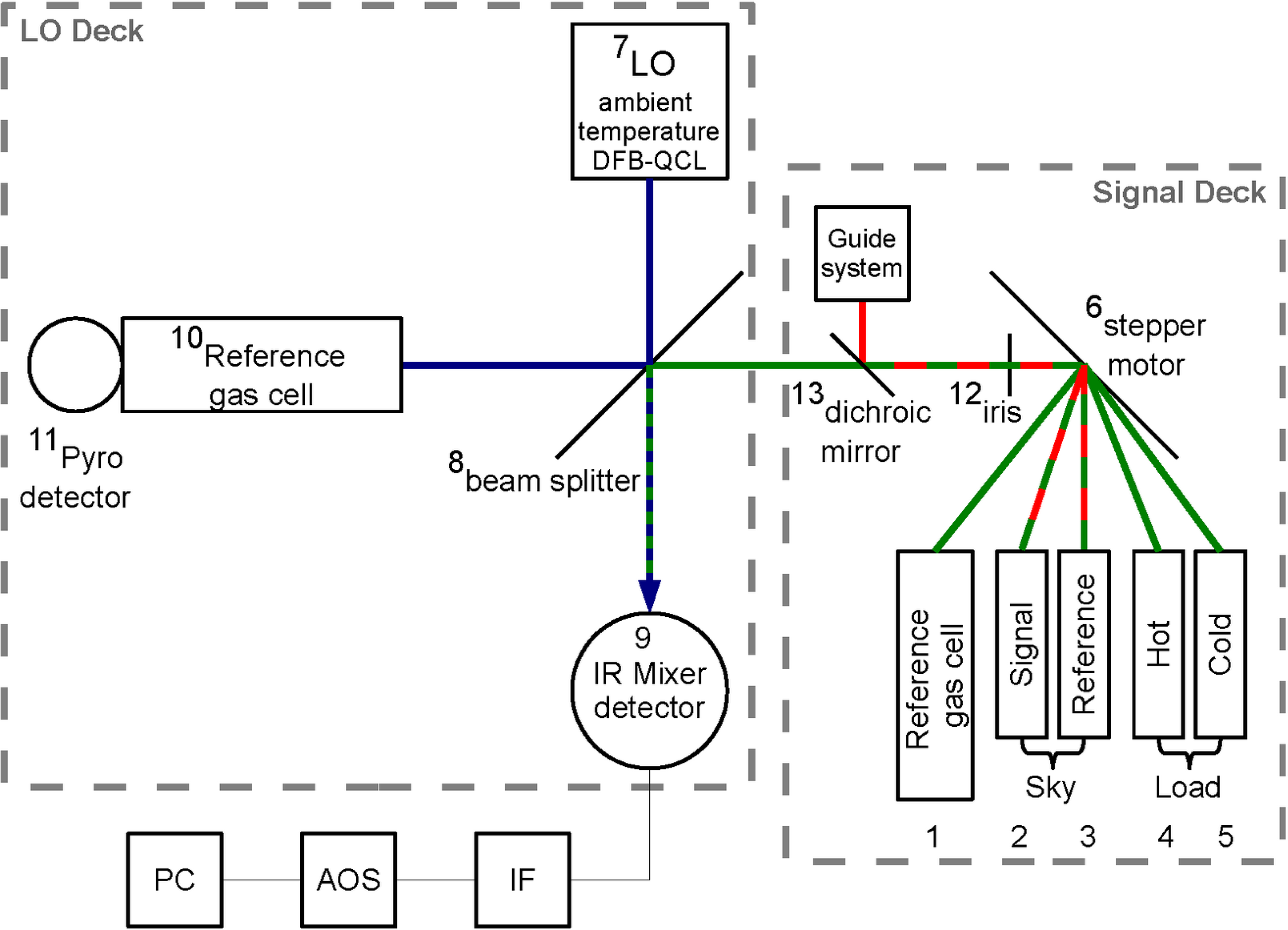
Figure 1.
Schematic view of the beam path in the spectrometer. The green line indicates the IR signal beam of the different sources (1–5) selected by the scanner mirror (6). The red line indicates the optical signal used for active tracking. The blue line indicates the local oscillator (LO) (7) output beam. The two IR beams are superimposed on the beam splitter (8) and imaged on the mixer (9). The reflected fraction of the LO beam is fed through a gas cell (10) onto the pyro detector (11) used for stabilization purposes. The mixer generates an intermediate frequency, which is processed (intermediate frequency (IF)) and analyzed (acousto-optical spectrometer (AOS)) with common radio astronomical components before it is archived and displayed (PC).
Signal Deck: On the upper, or signal, deck, four radiation sources, needed for calibration purposes, are located, which are a black body radiation source at 673 K as the hot load (4, Figure 1), a room temperature absorber as the cold load for intensity calibration (5, Figure 1), a steady state emitter observed through a reference gas cell for spectral calibration and (1, Figure 1) an input port for the atmospheric signal, provided by the telescope or heliostat, (2 + 3, Figure 1). The beam selection is provided by a commercially available stepper motor (6, Figure 1 Trinamic [21]). The stepper motor routes the various beam paths through an iris for alignment purposes. The iris (12, Figure 1) is located in the focal plane of the infrared detector (9, Figure 1). This is defined by an off-axis parabola (OAP) whose focal length has to be adjusted to the specific input optics. Additionally, a dichroic mirror (DM) (13, Figure 1) is introduced into the beam to separate the incoming visible and infrared light. The visible signal can be used for active tracking. The infrared signal is forwarded towards the mentioned OAP. Additionally, a visible alignment laser is introduced into the beam path.
LO Deck: The lower deck of the instrument is called the LO deck. Here, the LO (7, Figure 1), as well as the infrared detector (9, Figure 1) and the setup of the LO stabilization circuit (10 + 11, Figure 1) are located along with the beam combining element (beam splitter) (8, Figure 1). The beam splitter is made of zinc selenite (ZnSe) and has a reflective surface coating with a reflection index of 90%. It is set up such that 90% of the IR signal to be analyzed is reflected onto the mixer, whereas 10% of the LO signal is transmitted, which is sufficient for LO shot noise limited detection.
A QCL operating in continuous wave single mode at room temperature is used as the LO. The device provides an output power of approximately 30 mW and a continuous spectral tuning range of approximately 1% around the central wavenumber [18,19]. Such QCLs have recently replaced gas lasers as a state-of-the-art LO in infrared heterodyne spectroscopy [1]. Currently, two different custom-made QCLs, emitting at 7.8 μm (∼ 1,285 cm−1), from Alpes Lasers [22] and 8.6 μm (∼ 1,160 cm−1) from Maxion Technologies [23], are available for application.
The mixer is a mercury cadmium telluride (MCT)-doped semiconductor pin-photo diode optimized for heterodyne detection between 7.8 μm (∼ 1,285 cm−1) and 12.0 μm (830 cm−1). The diode must be operated at liquid nitrogen temperature of 77 K and has to be biased between 0.5 V and 1.0 V. The mixer has a maximum quantum efficiency of approximately 50%.
The Signal Processing: The IF signal, generated by the heterodyne mixer, is amplified and shifted to the frequency range of the backend acousto-optical spectrometer (AOS), which is tuned to be sensitive from 250 MHz to 1,650 MHz. It possess a fluctuation bandwidth δfl of 1.3 MHz and an IF bandwidth B of 1.4 GHz, defining the IF bandwidth of the entire instrument. AOSs were developed and assembled at our institute [24] and have been applied successfully for many years for various purposes in the field of radio-astronomy and spectroscopy [1,25,26]. Further analysis and data processing is performed by a PC.
3. Performance of the Receiver
In the following sections, a theoretical approach on the frequency stabilization process of the LO, as well as laboratory measurements to characterize the receiver are presented. Emphasis is given to the verification of the spectral stability and sensitivity. A summary of all the relevant parameters of the receiver can be found in Table 1.

Table 1.
List of important specifications for Infrared Compact Heterodyne Instrument for Planetary Science (iChips).
3.1. Stabilization of the Local Oscillator
The frequency stability of the receiver is defined by the signal stability of the LO. Frequency shifts due to systematic and statistical effects, i.e., temperature drifts or fluctuations of the laser voltage, cause instabilities and line broadening on the detected signal.
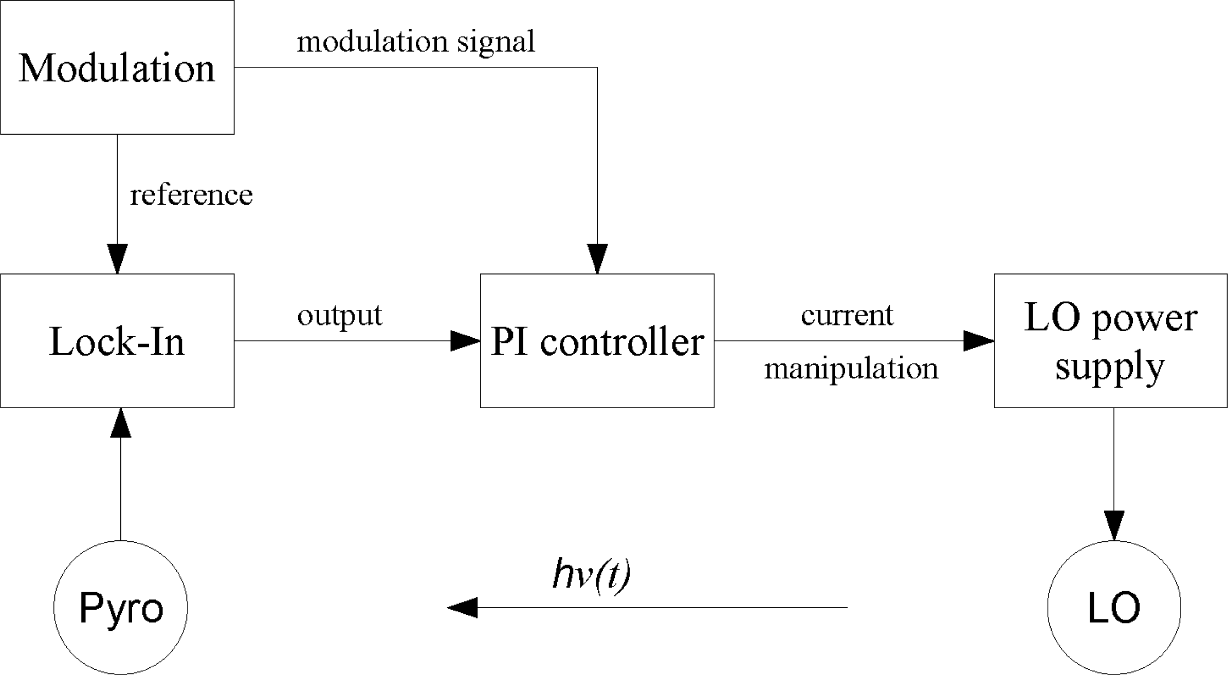
The powerful QCLs allow one to stabilize the LO output frequency by using the reflected fraction of the LO power (see the scheme in Figure 2). The radiation is fed through a cell, containing a reference gas, whose transition features (commonly, absorption lines) are detected on the pyro detector. A slight modulation of the LO frequency leads to a varying attenuation of the incident power. The output signal is evaluated by a lock-in amplifier, generating an error signal corresponding to the frequency offset from the tip of the absorption feature. A proportional-integral (PI) regulator processes and amplifies the error signal, which is finally fed back to the laser current supply to keep the laser frequency stable.

Figure 2.
Schematic view of the frequency stabilization circuit. The LO output beam is reflected to the beam splitter and then fed through a gas cell. The signal is detected and converted (pyro), analyzed and compared to the applied modulation (lock-in) and counteracted (proportional-integral (PI)) to keep the LO frequency stable by the current manipulation.
3.2. Influence of the Modulation on the Line Width
Although the modulation of the LO operating current is essential for the stabilization circuit, it increases the effective spectral width of any narrow feature. Thus, a detailed analysis of the influence of the modulation on the spectral line is essential.
The spectral line shape of the LO output obeys a Gaussian function (comp. Equation (A1) in Appendix A), in which νc is the center frequency of the Gaussian distribution. By applying a modulation to the LO, the absolute LO current, ILO, can be split into an initial current at rest, I0, and a time-variant oscillating modulation part, Ios(t)
The current change is proportional to the change in frequency within the modulation amplitude, and the center position for the Gaussian distribution, νc, which is now time-variant, too, has to be substituted by νc(t). Hence, the amplitude of the current modulation corresponds to the bandwidth of the LO output frequency and is, for further reference, called modulation bandwidth Δν. The impact of the applied triangular wave modulation form (TWM) on the retrieved spectrum is investigated in detail.
The detected heterodyne signal can be understood as the spectral superposition of two lines. To describe the line shape of the resulting heterodyne signal, the time-dependent Gaussian function of the LO has to be convoluted with the constant signal of the detected line. A detailed calculation of the convolution of a time-dependent and a static Gaussian distribution can be found in Appendix A.
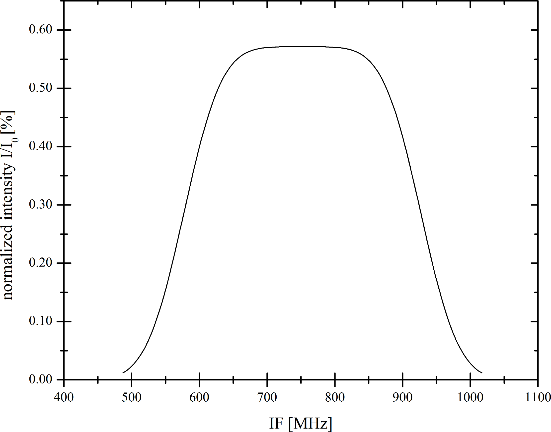
The time integral over a Gaussian function gives the error function (ERF), and the execution of the integral yields the final line shape of the detected heterodyne signal in dependence upon the modulation bandwidth, Δν. For a TWM, every Gaussian distribution within the modulation bandwidth at a time, t, has statistically the same weight. Thus, for increasing modulation bandwidth, the line disperses and forms a plateau around the center frequency. Simultaneously, the intensity decreases. An example of the intensity distribution of the resulting heterodyne spectrum for an overdimensioned modulation bandwidth is displayed in Figure 3. The line is normalized to the distribution of the resulting heterodyne line for an unmodulated LO with a full width at half maximum of FWHM0 = 100 MHz, and intensity, I0.
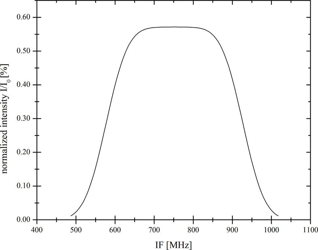
Figure 3.
Line shape of the heterodyne signal for a triangular wave modulation form (TWM) with Δν = 3.37 FWHM0. For a large modulation bandwidth, Δν, the line disperses and forms a plateau around its center frequency.
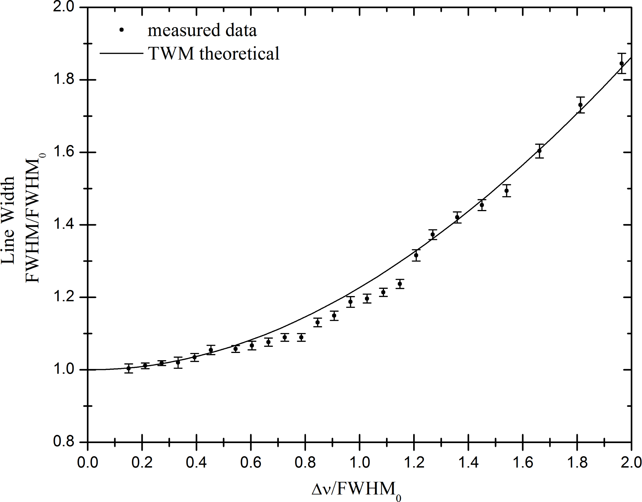
Comparison: In Figure 4, the increase of the FWHM in units of the width of the unmodulated line, FWHM0 = 100 MHz, is plotted for a theoretical determination of a TWM. For modulation bandwidths that are small compared to FWHM0, the broadening effect is negligible. A modulation bandwidth of 0.50 FWHM0, has an influence of only a few percent on the line width. To verify these theoretical determinations, the laser was stabilized on a CH4 absorption line (ν̄CH4 = 1,286.564 cm−1) to measure a close-by N2O reference line (ν̄N2O = 1,286.569 cm−1), and heterodyne spectra of N2O at 25 different modulation settings were taken for a TWM. Gaussian distributions were fitted to the resulting lines. At least 30 spectra with a total integration time of 300 s were measured and averaged for each modulation amplitude. The results are displayed as black dots in Figure 4. The LO output frequency is, in the first order, proportional to the current amplitude and can be described as Δν = −γΔI. The tuning rate, γ, was calibrated to be
. Figure 4 shows an excellent agreement between calculations and measurements of the increase of the resulting heterodyne line width. For a known modulation bandwidth, the original line width can be derived from observations. The smallest modulation bandwidth was ≈0.15 FWHM0, which affects the resulting line width by less than 0.5%.

Figure 4.
Measured line widths (dots) compared to theoretical course (solid line) for an increasing modulation bandwidth, Δν, of a TWM.
3.3. Spectral Stability
The center position of the heterodyne line was measured for 5,400 s to investigate the spectral stability of the LO. These measurements were performed using the QCL emitting at 7.8 μm (∼ 1,285 cm−1). The stabilization was set up as described in Section 3.2. Again, a Gaussian line profile was fitted to the measured line after each measuring cycle, and the center position of the N2O reference line was investigated. The absolute frequency calibration of the AOS was achieved by fitting a series of lines provided by a comb generator with a defined spectral distance of 50 MHz after each scan. The AOS’s thermal stability during each scan was uncritical, since frequency drifts of less than 1 MHz per day are common.
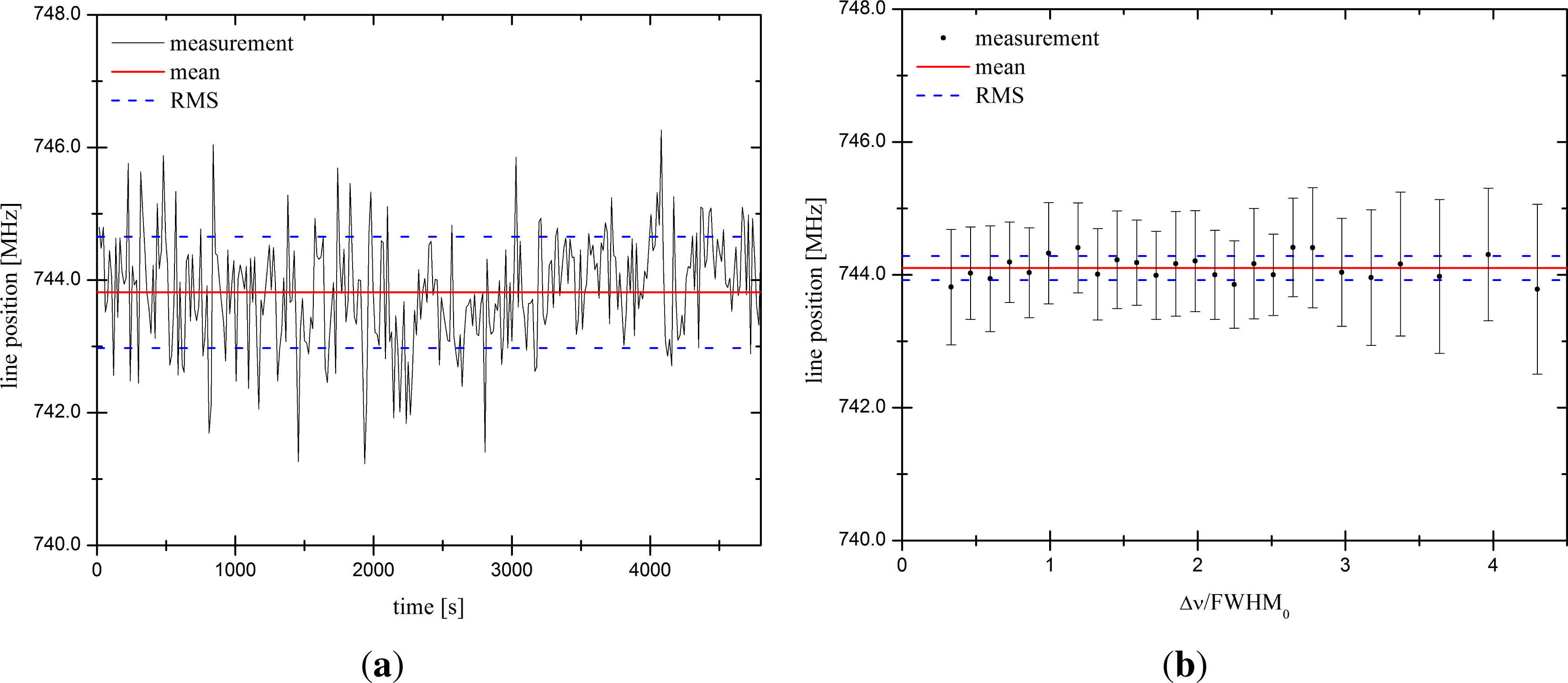
Figure 5a displays the variation in time of the center frequency of the heterodyne line for one single modulation bandwidth, Δν= 0.33 FWHM0 (FWHM0 = 48 MHz). The standard deviation of the measured line position is σm = 0.84 MHz. The line position was stable during the observation. In Figure 5b, the line positions for increasing modulation bandwidth of a TWM are plotted. The data points represent the average of at least 30 spectra per modulation bandwidth. As expected, the line position is independent from the modulation bandwidth. The standard deviation is σ = 0.35 MHz. Both errors are smaller than the AOS fluctuation bandwidth (δfl = 1.3 MHz), proving a resolving power of
.
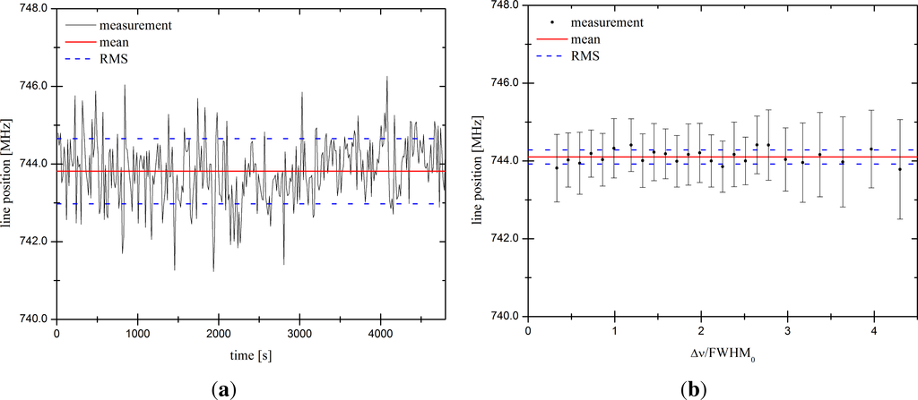
Figure 5.
The variation of the center frequency of the measured heterodyne line is displayed. The red horizontal line represents the mean value and the blue dashed horizontal lines its RMS. (a) The center frequency is plotted vs. the observing time with a constant modulation bandwidth of Δν= 0.33 FWHM0. This measurement corresponds to the first data point in (b); (b) The center frequency is plotted vs. the modulation bandwidth of a triangular wave modulation (TWM), normalized to the FWHM0 of the unmodulated line.
3.4. Allan Variance Measurement
A key factor for astronomical and terrestrial observations is the amplitude stability of the receiver. Its variance, σ, must decrease with increasing integration time, τ (radiometric behavior) [27]. The Allan variance method, a common procedure to investigate the accuracy of time and frequency standards [28], is used to demonstrate the radiometric decrease of the noise amplitude. The minimum of the Allan variance can be determined using a power law, where frequency drifts are proportional to τβ and the white noise contribution is proportional to
[29]. It can be written as:
Hence, when the variance is plotted on a logarithmic scale, the −1 slope defines the time interval in which the radiometer equation must be valid.
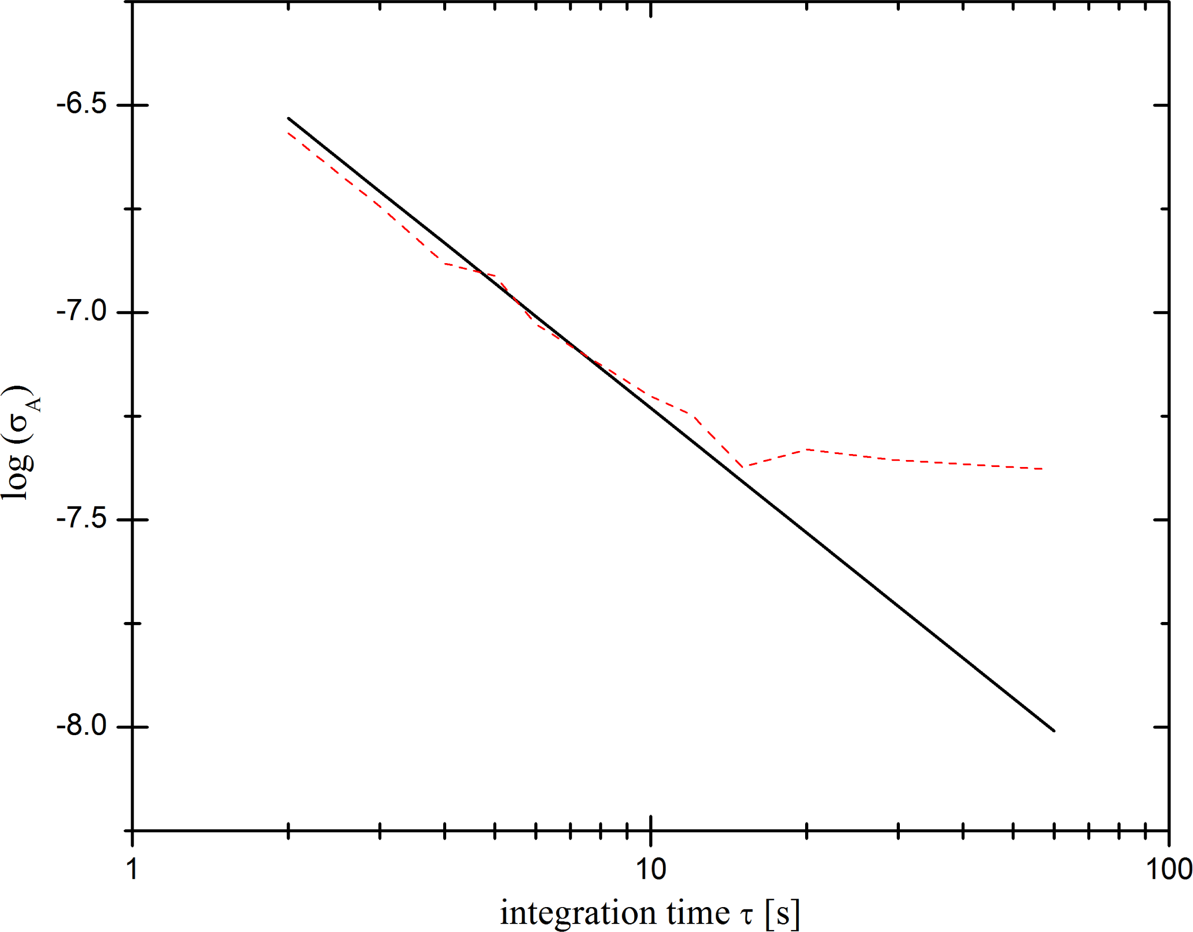
In Figure 6, the radiometric behavior of the noise amplitude can be observed. The variance of the data is plotted over the integration time of 60 s. The noise amplitude decreases with a slope of −1 for a time interval of ≈10 s, which defines the maximum integration time for one cycle, τcyc.
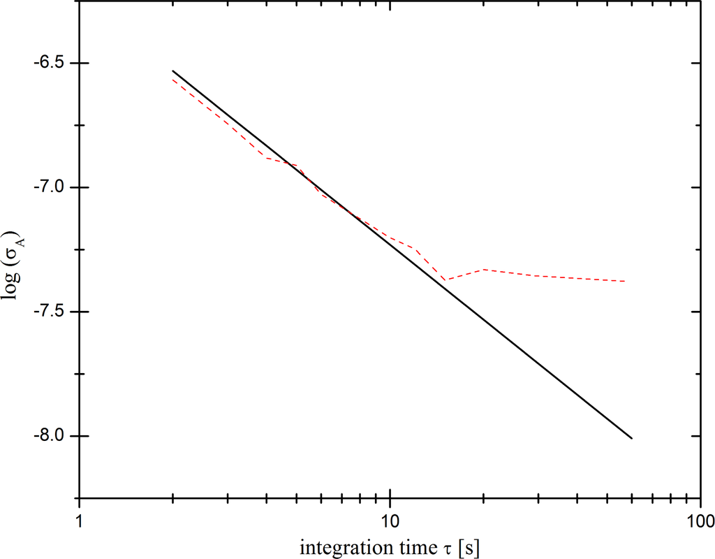
Figure 6.
The variance of the noise amplitude is plotted vs. the integration time on a double logarithmic scale. The black line represents the theoretical decrease for pure white noise. The red line represents the measurement. The minimum of the variance can be found at an integration time, ≈10 s. Within this time interval, the noise amplitude decreases radiometrically.
3.5. Sensitivity
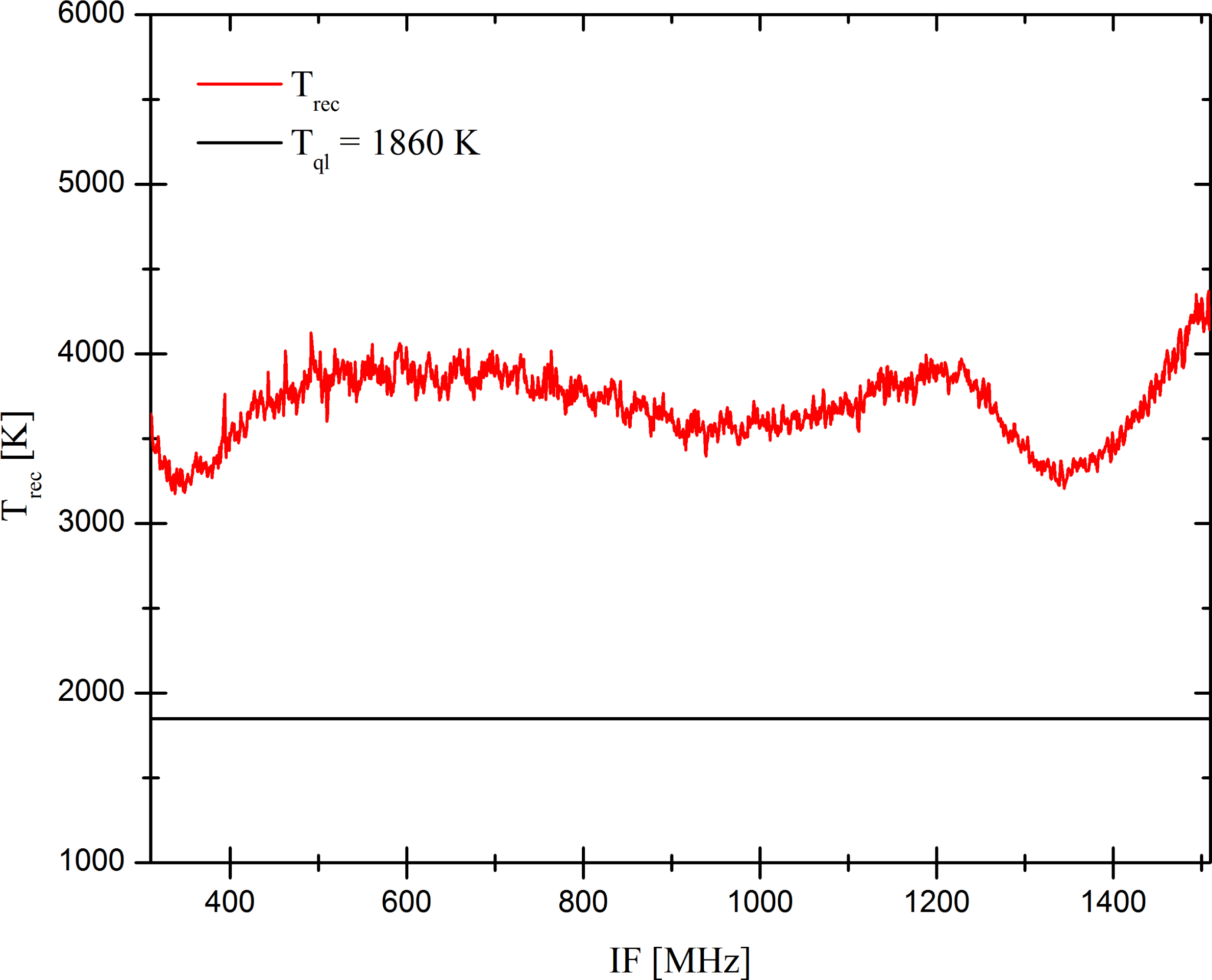
The sensitivity of a heterodyne receiver is best described by the receiver noise temperature, Trec [30]. It was determined to be ≈ 3,700 K. In Figure 7, Trec and the quantum limit Tql (1,860 K at 7.8 μm) are plotted vs. the detector bandwidth. Taking the detectors quantum efficiency of approximately 70% and the optical losses (≥25%, including 10% transmission losses of the beam splitter) into account, the minimum achievable system temperature calculates to ∼3,600 K. Thus, the system temperature coincides by 97% with the quantum limit, which is an exceptional good value for any heterodyne receiver.

Figure 7.
The sensitivity of the instrument from 300 MHz to 1,500 MHz is displayed in terms of the receiver noise temperature, Trec. The red line displays the measured performance, which is within a factor of two of the quantum limit represented by the black line. QCL, quantum cascade lasers.
4. Demonstration of Observing Modes: Atmospheric Measurements
As mentioned, the instrument can be operated in two different modes, the staring mode and the scanning mode. Measurements to illustrate the instrument’s capability for atmospheric observation were performed.
To obtain a calibrated spectrum, the ratio of the incident signals from all observed sources is determined:
where H: hot calibration load, C: cold calibration load, S: sky signal, R: sky reference and ν̄: wavenumber of observed radiation [1]. The retrieved dimensionless spectrum, F, is then multiplied with the difference of the brightness temperature from a hot load and a cold load (TH− TC). For hot sources, like the sun, the sky reference, R, may be substituted by the cold calibration load, C.
4.1. Staring Mode: Observation of Atmospheric Ozone Features
In staring mode, the LO frequency needs to be stabilized onto an absorption line (see Section 3.1) to investigate single molecular transition features with ultra high resolution of
. A reference line is measured simultaneously to each data set during observation, required for absolute frequency calibration and to verify the stability of the LO spectral line, as demonstrated in Section 3.3.
A possible application for the staring mode is the retrieval of atmospheric dynamics. For demonstration purposes, middle atmospheric terrestrial ozone (O3) features were investigated. Since the ozone layer has its peak density at approximately 30 km altitude, the lines are sufficiently narrow to be observed. Initial observations were performed on 10 February 2012, at the I. Physikalisches Institute of the University of Cologne. An ozone line at 1,162.914 cm−1 was observed in absorption, using the sun as the background radiation source. A commercially available solar tracker was used as the heliostat.
During one measuring cycle, the integration time, τcyc, has to be distributed into appropriate exposure times on each source to minimize the RMS, hence optimizing the signal-to-noise ratio (SNR). The exposure time on the single source can be flexibly adjusted to the specific observational condition. For observations in solar occultation mode, a signal integration time of
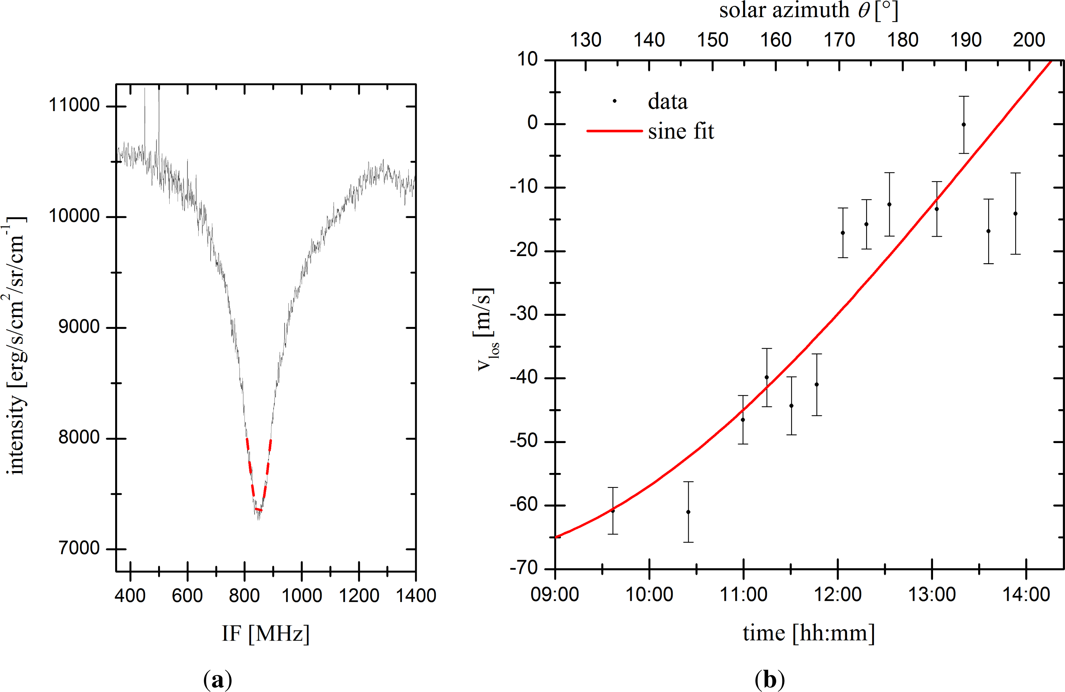
is adequate. One example of a measured O3 absorption line, for a sum of 100 cycles with τcyc ≈ 3 s, is displayed in Figure 8a. SO2 at ≈1 mbar was used as reference to stabilize the LO at 1,162.886 cm−1. A triangular wave modulation with a bandwidth of Δν = 0.25 FWHM0, with FWHM0 = 70 MHz, was applied. In a first step, a Voigt profile was fitted to the line tip (±50 MHz around the expected IF value) of each measurement to retrieve the precise center frequency of the lines. Thirteen different measurements were performed within 270 min. The shift between the rest IF of the O3 transition (νIF,theo in MHz) and the measured IF (νIF,meas) yields the line of sight (LoS) component of the wind velocity (vlos) in the stratosphere.
where νO3 is the absolute frequency of the observed transition. Errors are calculated via Gaussian error propagation from 1-σ fitting errors and found to be between 0.30 MHz ≤ Δνmeas≤ 0.55 MHz for all fits. Thus, fitting errors are smaller than the spectral resolution of the backend spectrometer. In Figure 8b, the retrieved LoS wind velocities are plotted. In our case, a Doppler shift to a lower frequency yields a negative LoS wind, implying a wind moving away from the observer and vice versa. LoS wind velocities increase from (−60.8 ± 3.6) m·s−1 at 9:36 h local time (LT) to (−0.1 ± 4.5) m·s−1 at 13:20 h LT, mainly due to the change in observing geometry.

Figure 8.
Measured O3 Line and Line of Sight Wind Velocity. (a) One example of a measured O3 absorption line at an IF of 849.6 MHz (black) and the Voigt fit to the line peak (red); (b) Resulting line of sight wind velocities from the Doppler shifted peak positions of the absorption line plotted vs. the observing time and corresponding solar azimuth, θ. The fit error is represented by the error bars. A sine function with a period of 24 h was fitted to the data.
For further interpretation, a constant horizontal wind field during the time of observation was assumed. The horizontal wind can then be derived by taking the observing geometry into account. Following the sun, a sine wave behavior with a 24 h period of the retrieved LoS wind velocities, in dependency of elevation (ϕ) and the azimuth (θ), is expected, by neglecting any up- and down-ward propagation. At the point where the LoS wind velocity is zero, the wind field is perpendicular to the observer (θvlos=0). Thus, the resulting horizontal wind, vh, can be expressed as:
A sine fit was applied to the data presented in Figure 8b. The horizontal wind velocity was found to be vh = 60.3 ± 4.4 m·s−1. The uncertainty of the rest frequency of the observed O3 feature is unreported (Hitran [31]), which might lead to an offset.
Additionally, in order to investigate a vertically distributed wind in dependence of the altitude, a careful analysis of the full line shape has to be accomplished. Due to the radiative transfer through the atmosphere, different pressure layers, in terms of broadening effects, have a different influence on the spectral shape of the line. This method is successfully applied by Rüfenacht et al. [14]. Thus, the tip of the line originates in a specific pressure layer in the Earth’s atmosphere.
4.2. Scanning Mode: Observation of Terrestrial Transmission
The second observing mode of the instrument is the scanning mode. The QCL is capable of sweeping continuously through its whole spectral tuning range (∼ 5–6 wavenumber, depending on the operating temperature) within several seconds. This enables scanning the atmospheric transmission within a short time span.
First measurements using the scanning mode were performed during an observing campaign in June 2011, at the McMath-Pierce Solar Telescope East Auxiliary at Kitt Peak National Observatory in Arizona, USA. In Figure 9, the measured atmospheric transmission between ∼ 1,282.0 cm−1 and ∼1,287.5 cm−1 is displayed. The data were acquired by rectifying the heterodyne signal using a Schottky-barrier diode with a bandwidth of approximately 1.4 GHz. The total integration time was 360 s. The solar zenith angle (SZA) for the measurement was 41°, corresponding to an airmass of 1.3 (an airmass of one corresponds to zenith observations). The obtained transmission spectrum is compared to the mid-summer latitude atmosphere model [32]. The model spectrum was computed using the online database spectralcalc [33]. Since the atmospheric parameters during observation (i.e., water abundance, air pressure, etc.), were not fully known, a set of standard values was taken to acquire the model. This is the main reason for any intensity deviation of the model from the data. Another, yet neglected, effect is the temperature change of the LO, which affects the output frequency during the scan, yielding small systematic shifts in the spectrum. Nevertheless, absorption features of methane, water and nitrous oxide can be unambiguously assigned.
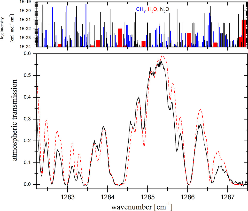
Figure 9.
(Top) Molecular transitions of the, in the probed spectral range predominant, atmospheric constituents, nitrous oxide, N2O (black), water, H2O (red), and methane, CH4 (blue). (Bottom) The atmospheric transmission above the McMath-Pierce Solar Telescope (black) compared to the mid-summer latitude model of the terrestrial atmosphere (red).
Further progress will be made to optimize this application mode by implementing variable spectral resolution and instantaneous calibration, taking thermal drifts of the LO into account.
5. Discussion
Room temperature QCLs were successfully applied as LOs in a heterodyne spectrometer for the first time. Spectral analysis of trace gases can be conducted in two different operational modes.
Initial measurements in staring mode of LoS wind velocities were performed by probing stratospheric ozone. The presented results are yet preliminary, since the accuracy of the rest of the frequency of the observed ozone line is unreported. Assuming good knowledge about the observed transition, the horizontal wind can be calculated by considering the observing geometry. Ground-based remote sensing wind measurements in the lower terrestrial stratosphere are quite rare, but have recently been performed by Rüfenacht et al. [14] using a microwave spectrometer. Hence, infrared heterodyne spectroscopy can provide complementary studies for ground-based observations on the dynamics in the telluric stratosphere. The observed lines originate in an altitude region around 30 km, where the ozone layer has its peak density. However, a sophisticated retrieval algorithm has to be established, in order to obtain information on the exact observing altitude. Nevertheless, initial observations prove the feasibility of the instrument for the investigation of stratospheric dynamics.
The usage of tunable room temperature QCLs allows one to scan the terrestrial atmosphere over several wavenumbers. A first transmission spectrum, taken at around 7.8 μm (∼ 1,285 cm−1), is, in principle, in agreement with an average mid-summer latitude atmosphere model [32] and proves the general performance of the instrument for this operational mode. By using the scanning mode, highly pressure broadened methane transition can be observed with a high spectral resolution and good SNR. Although, the Schottky-barrier diode, used for the initial measurements, limits the resolution to its intrinsic bandwidth. Future work will be performed to discard the diode and to establish the AOS for data acquisition in the scanning mode, enabling the possibility to increase the resolution of the spectra by averaging over an arbitrary and adjustable frequency range (≤340 MHz) easily to
Additionally, a careful frequency calibration will be performed by simultaneously measuring a reference gas, comparable to the staring mode calibration.
The scanning mode offers the capability to scan the terrestrial atmosphere within a few minutes. Thus, ground-based observing campaigns may provide valuable and continuous input on the distribution of terrestrial methane. From the line shape and the depth of the absorption, it is possible to retrieve an abundance of methane in different altitudes using an inversion method, given a decent knowledge of additional atmospheric parameters, like atmospheric temperatures. With an SNR of 1,000, an accuracy of 0.1 ppmv can be achieved if the temperature and water vapor profile is known [34].
Besides the molecules mentioned above, many more molecular transitions in the mid-infrared wavelength regime are accessible. Measurements of sulfur and carbon dioxide (SO2, CO2), nitrous oxide (N2O) and ethylene (C2H4) are just some examples of such gases.
In comparison to radiosondes, a tunable heterodyne spectrometer provides a relatively easy and cost-efficient ground-based technique for long-term monitoring of atmospheric parameters.
6. Conclusions
In the present paper the setup of a new compact infrared heterodyne receiver, named iChips, is specified. iChips is the first infrared heterodyne receiver using room temperature quantum cascade lasers as local oscillators. Two different operating modes honor the instrument.
In the staring mode, iChips can be used to observe single fully resolved molecular features. This is demonstrated by the observation of a telluric ozone line around 8.6 μm (∼ 1,160 cm−1). Due to the ultra high spectral resolution of
, such lines can be used to retrieve Doppler winds by determination of the precise frequency position. Applying the second operation mode, the scanning mode iChips can be used to cover a broader wavelength region with resolution,
. Demonstrative measurements of the terrestrial atmosphere around 7.8 μm (∼1,285 cm−1) are shown.
The results validate the capability of iChips for observations of terrestrial and extraterrestrial atmospheres. The instrument’s compactness allows its deployment in flexible field measurement campaigns, even in remote locations, and a broad range of applications for the instrument is available. Further observations of terrestrial ozone to track abundances and stratospheric dynamics and the observation of terrestrial methane are planned.
Acknowledgments
We would like to thank Claude Plymouth and Eric Galayda, staff of the McMath-Pierce Solar Telescope at Kitt Peak National Observatory during the observing campaign in 2011, for their great support and input. Additionally, we would like to thank Mario Zacharias, Institute for Theoretical Physics, University of Cologne, for his support on Mathematica 8.
Conflict of Interest
The authors declare no conflict of interest.
References
- Sonnabend, G.; Wirtz, D.; Schieder, R. Tuneable Heterodyne Infrared Spectrometer for atmospheric and astronomical studies. Appl. Opt 2002, 41, 2978–2984. [Google Scholar]
- Kostiuk, T.; Fast, K.E.; Livengood, T.A.; Hewagama, T.; Goldstein, J.J.; Espenak, F.; Buhl, D. Direct measurement of winds of Titan. Geophys. Res. Lett 2001, 28, 2361–2364. [Google Scholar]
- Kostiuk, T.; Hewagama, T.; Fast, K.E.; Livengood, T.A.; Annen, J.; Buhl, D.; Sonnabend, G.; Schmlling, F.; Delgado, J.D.; Achterberg, R. High spectral resolution infrared studies of Titan: Winds, temperature, and composition. Planet. Space Sci 2010, 58, 1715–1723. [Google Scholar]
- Sornig, M.; Sonnabend, G.; Stupar, D.; Kroetz, P.; Nakagawa, H.; Mueller-Wodarg, I. Venus upper atmospheric dynamical structure from ground-based observations shortly before and after Venus inferior conjunction 2009. Icarus 2012, 225, 828–839. [Google Scholar]
- Sornig, M.; Livengood, T.A.; Sonnabend, G.; Stupar, D.; Krötz, P. Direct wind measurements from November 2007 in venus upper atmosphere using ground-based heterodyne spectroscopy of CO2 at 10 μm wavelength. Icarus 2012, 217, 863–874. [Google Scholar]
- Sonnabend, G.; Krötz, P.; Schmülling, F.; Kostiuk, T.; Goldstein, J.; Sornig, M.; Stupar, D.; Livengood, T.; Hewagama, T.; Fast, K.; Mahieux, A. Thermospheric/mesospheric temperatures on Venus: Results from ground-based high-resolution spectroscopy of CO2 in 1990/1991 and comparison to results from 2009 and between other techniques. Icarus 2012, 217, 856–862. [Google Scholar]
- Sonnabend, G.; Sornig, M.; Kroetz, P.; Stupar, D. Mars mesospheric zonal wind around northern spring equinox from infrared heterodyne observations of CO2. Icarus 2012, 217, 315–321. [Google Scholar]
- Fast, K.; Kostiuk, T.; Hewagama, T.; A’Hearn, M.F.; Livengood, T.A.; Lebonnois, S.; Lefèvre, F. Ozone abundance on Mars from infrared heterodyne spectra. Icarus 2006, 183, 396–402. [Google Scholar]
- Ortland, D.A.; Skinner, W.R.; Hays, P.B.; Burrage, M.D.; Lieberman, R.S.; Marshall, A.R.; Gell, D.A. Measurements of stratospheric winds by the high resolution Doppler imager. J. Geophys. Res. Atmos 1996, 101, 10351–10363. [Google Scholar]
- Baron, P.; Murtagh, D.P.; Urban, J.; Sagawa, H.; Ochiai, S.; Körnich, H.; Khosrawi, F.; Kikuchi, K.; Mizobuchi, S.; Sagi, K.; et al. Observation of horizontal winds in the middle-atmosphere between 30°S and 55°N during the northern winter 2009–2010. Atmos. Chem. Phys. Discuss 2012, 12, 32473–32513. [Google Scholar]
- Reitebuch, O.; Lemmerz, C.; Nagel, E.; Paffrath, U.; Durand, Y.; Endemann, M.; Fabre, F.; Chaloupy, M. The airborne demonstrator for the direct-detection doppler wind lidar ALADIN on ADM-Aeolus. Part I: Instrument design and comparison to satellite instrument. J. Atmos. Ocean. Technol 2009, 26, 2501–2515. [Google Scholar]
- Shepherd, G.; McDade, I.; Gault, W.; Rochon, Y.; Scott, A.; Rowlands, N.; Buttner, G. The stratospheric wind interferometer for transport studies (swift). Adv. Space Res 2001, 27, 1071–1079. [Google Scholar]
- Hildebrand, J.; Baumgarten, G.; Fiedler, J.; Hoppe, U.P.; Kaifler, B.; Lübken, F.J.; Williams, B.P. Combined wind measurements by two different lidar instruments in the Arctic middle atmosphere. Atmos. Meas. Tech 2012, 5, 2433–2445. [Google Scholar]
- Rüfenacht, R.; Kämpfer, N.; Murk, A. First middle-atmospheric zonal wind profile measurements with a new ground-based microwave Doppler-spectro-radiometer. Atmos. Meas. Tech 2012, 5, 2647–2659. [Google Scholar]
- Ehret, G.; Flamant, P. French-German Methane Monitoring Satellite MERLIN. Proceedings of the 39th COSPAR Scientific Assembly, Mysore, India, 14–22 July 2012; 39, p. 505.
- Pougatchev, N.S.; Connor, B.J.; Rinsland, C.P. Infrared measurements of the ozone vertical distribution above Kitt Peak. J. Geophys. Res.-Atmos 1995, 100, 16689–16697. [Google Scholar]
- Griffith, D.W.T.; Jones, N.B.; McNamara, B.; Walsh, C.P.; Bell, W.; Bernardo, C. Intercomparison of NDSC ground-based solar FTIR measurements of atmospheric gases at lauder, New Zealand. J. Atmos. Ocean. Technol 2003, 20, 1138–1153. [Google Scholar]
- Faist, J.; Capasso, F.; Sivco, D.L.; Sirtori, C.; Hutchinson, A.L.; Cho, A.Y. Quantum cascade laser. Science 1994, 264, 553–556. [Google Scholar]
- Beck, M.; Hofstetter, D.; Aellen, T.; Faist, J.; Oesterle, U.; Ilegems, M.; Gini, E.; Melchior, H. Continuous wave operation of a mid-infrared semiconductor laser at room temperature. Science 2002, 295, 301–305. [Google Scholar]
- Weidmann, D.; Reburn, W.J.; Smith, K.M. Ground-based prototype quantum cascade laser heterodyne radiometer for atmospheric studies. Rev. Sci. Instrum 2007, 78, 073107. [Google Scholar]
- TRINAMIC Motion Control GmbH & Co. KG. Available online: http://www.trinamic.com (accessed on 1 February 2013).
- ALPES LASERS Quantum Cascade Solutions. Available online: http://www.alpeslasers.ch/ (accessed on 1 March 2013).
- MAXION Technologies, Inc. Available online: http://www.maxion.com/ (accessed on 1 March 2013).
- Schieder, R.; Tolls, V.; Winnewisser, G. The cologne acousto optical spectrometers. Exp. Astron 1989, 1, 101–121. [Google Scholar]
- De Graauw, T. The herschel-heterodyne instrument for the Far-Infrared (HIFI). Astron. Astrophys 2010, 518, L6. [Google Scholar]
- Heyminck, S.; Graf, U.U.; Güsten, R.; Stutzki, J.; Hübers, H.W.; Hartogh, P. GREAT: The SOFIA high-frequency heterodyne instrument. Astron. Astrophys. 2012. [Google Scholar] [CrossRef]
- Waters, J.; Janssen, M. Fundamentals. In Atmospheric Remote Sensing by Microwave Radiometry; Wiley: New York, NY, USA, 1993; Chpater 1.3.1; pp. 383–496. [Google Scholar]
- Allan, D. Statistics of atomic frequency standards. Proc. IEEE 1966, 54, 221–230. [Google Scholar]
- Schieder, R.; Kramer, C. Optimization of heterodyne observations using Allan variance measurements. Astron. Astrophys 2001, 373, 746–756. [Google Scholar]
- Kraus, J.D.; Tiuri, M.; Carr, T.D. Radio Astronomy, 2nd ed.; Cygnus-Quasar Books: Powell, OH, USA, 1986. [Google Scholar]
- Rothman, L.; Gordon, I.; Barbe, A.; Benner, D.; Bernath, P.; Birk, M.; Boudon, V.; Brown, L.; Campargue, A.; Champion, J.P.; et al. The HITRAN 2008 molecular spectroscopic database. J. Quant. Spectrosc. Radiat. Transf 2009, 110, 533–572. [Google Scholar]
- Kantor, A.; Cole, A. Mid-latitude atmospheres, winter and summer. Geofisica Pura e Applicata 1962, 53, 171–188. [Google Scholar]
- SpectralCalc.com by GATS, Inc. Available online: http://www.spectralcal.com (accessed on 1 March 2013).
- Koide, M.; Taguchi, M.; Fukunishi, H.; Okano, S. Ground-based remote sensing of methane height profiles with a tunable diode laser heterodyne spectrometer. Geophys. Res. Lett 1995, 22, 401–404. [Google Scholar]
Appendix
A. Calculation for TWM
The spectral line shape of the LO output obeys a Gaussian function:
with σG representing the width of the line where the intensity dropped to
of the maximum.
For a triangular wave modulation (TWM) signal, the periodical frequency sweep can be described as:
with ν0 being the center frequency of the LO at rest, and the modulation bandwidth, Δν, has to be introduced to Equation (A1).
For a period, t ε [0, 2], the detected heterodyne signal can be understood as the spectral superposition of two beams. To describe the line shape of the resulting heterodyne signal, the time-dependent Gaussian function of the LO has to be convoluted with the constant signal of the detected line. Both signals are assumed to have a Gaussian shape. We receive:
where μ represents the new frequency axis, νline is the center frequency and σline is the Gauss width of the transition line.
The intensity of the resulting line can be described as the timely weighted average of the distribution. Integration of Equation (A3) over a full period, using the substitution,
, gives:
The calculations were performed with the program Mathematica 8 for different Δν.

© 2013 by the authors; licensee MDPI, Basel, Switzerland This article is an open access article distributed under the terms and conditions of the Creative Commons Attribution license (http://creativecommons.org/licenses/by/3.0/).