Estimation of Tree Lists from Airborne Laser Scanning Using Tree Model Clustering and k-MSN Imputation

Abstract

Individual tree crowns may be delineated from airborne laser scanning (ALS) data by segmentation of surface models or by 3D analysis. Segmentation of surface models benefits from using a priori knowledge about the proportions of tree crowns, which has not yet been utilized for 3D analysis to any great extent. In this study, an existing surface segmentation method was used as a basis for a new tree model 3D clustering method applied to ALS returns in 104 circular field plots with 12 m radius in pine-dominated boreal forest (64°14′N, 19°50′E). For each cluster below the tallest canopy layer, a parabolic surface was fitted to model a tree crown. The tree model clustering identified more trees than segmentation of the surface model, especially smaller trees below the tallest canopy layer. Stem attributes were estimated with k-Most Similar Neighbours (k-MSN) imputation of the clusters based on field-measured trees. The accuracy at plot level from the k-MSN imputation (stem density root mean square error or RMSE 32.7%; stem volume RMSE 28.3%) was similar to the corresponding results from the surface model (stem density RMSE 33.6%; stem volume RMSE 26.1%) with leave-one-out cross-validation for one field plot at a time. Three-dimensional analysis of ALS data should also be evaluated in multi-layered forests since it identified a larger number of small trees below the tallest canopy layer.

1. Introduction

Many modern systems for forest management planning require information at the individual tree level [1–4] or, at least, about the distribution of stem diameters at breast height (DBH) [5]. For the purpose of forest resource planning, unbiased estimates are also essential.

Data from airborne laser scanning (ALS) are three-dimensional coordinate measurements of light reflections from the ground and other objects. During the last fifteen years, methods have been developed to use ALS data for estimation of forest variables such as tree height and stem volume. The most commonly used method is estimation at an area level when forest variables measured in field plots are modeled from variables derived from ALS data for the same area [6]. The variables derived from the ALS data are typically measures of the height distribution and the density of the ALS data in different height intervals above the ground. The estimation is usually done with regression models [6] or with semi-parametric models such as k-Most Similar Neighbours (k-MSN), where the similarity is based on canonical correlations [7].

If the ALS data are dense enough, individual tree crowns (ITC) may also be delineated from the data. This has mostly been done based on surface models [8–10], such as a normalized digital surface model (nDSM). Typically, the local maxima in the surface model are defined as tree tops and the area around them is delineated to define tree crowns [11]. Features extracted from the spatial distribution or the intensity values of the ALS data inside each segment may be used to estimate stem volume and tree species of the individual trees [12–14]. This kind of analysis utilizes more details of the ALS data together with the knowledge of the shapes and proportions of tree tops and tree crowns. However, it often fails to detect trees standing close together and trees below the tallest canopy layer [10,15].

The failure of ITC segmentation to detect all trees has been addressed with statistical approaches. Maltamo et al.[16] used expected tree size distribution functions to predict small trees. Lindberg et al.[17] classified the delineated segments to determine the number of trees contained in each segment. The properties of the trees contained in each segment were estimated with regression from the properties of the ALS data in the segment. The resulting tree list in each field plot was then adjusted using the estimated stem volume and distributions of DBH and tree height in the field plot. Holmgren et al.[18] used imputation to estimate tree lists based on properties of the ALS data in the segment using harvester data as training data. For estimation of several correlated variables, it is difficult to fit parametric models. Breidenbach et al.[19] used a similar imputation approach to determine the properties of the trees contained in each segment, which they named the semi-ITC approach. The results were not significantly biased and more accurate than estimates from regression models at area level. ITC segmentation makes use of the 3D structure of the ALS data and can be based on models of tree crowns, while estimation at an area level usually only considers the vertical distribution and density of the ALS data [20].

Since the laser pulses can pass through gaps in the canopy, the ALS data include measurements of surfaces below the tallest canopy layer. This makes it possible to derive a digital elevation model of the ground also in dense forests [21,22]. Additionally, measurements may originate from small trees below the tallest canopy layer. These 3D properties have been used to delineate tree crowns from ALS data with clustering-based approaches where the initial values for the clustering are derived from local maxima in an nDSM or other means of detecting tree tops from the ALS data [23–27]. Other approaches have been to delineate tree crowns based on the mean shift algorithm [28] and to first determine an approximate number of tree stems by clustering of the ALS data below the tree crowns and then use the estimated stem number to delineate tree crowns with a normalized cut algorithm [29].

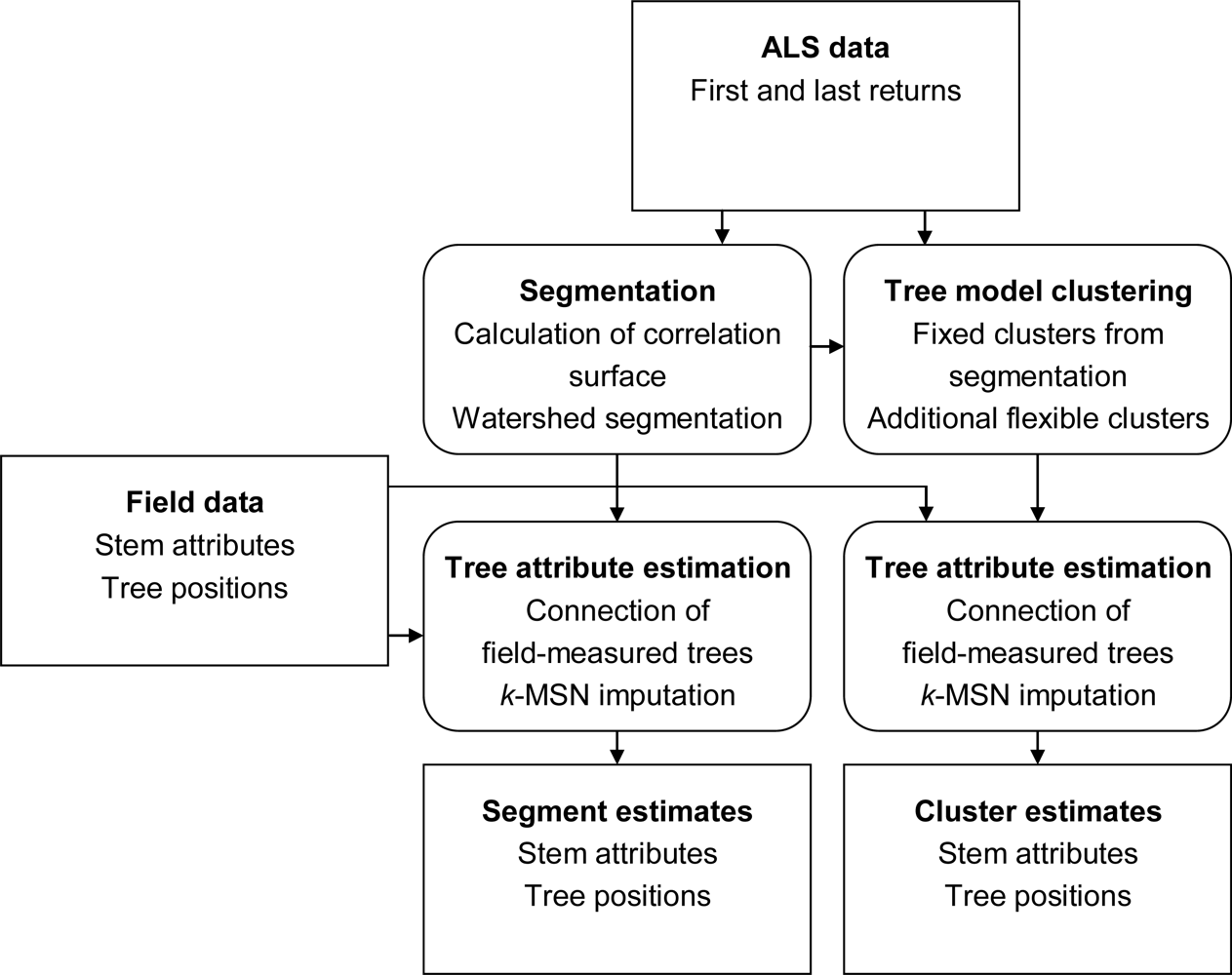
The aim of this study is to extract information from ALS data to estimate lists of individual trees with a higher accuracy when aggregated to area level than what is currently achieved with ITC segmentation of surface models. The idea is to first derive information about the tallest canopy layer from segmentation of a surface model and then use 3D analysis to extract information about trees below the tallest canopy layer with a tree model clustering approach. The information extracted from the ALS data is connected to field data to create models for unbiased plot level estimates of forest variables. The connection and estimation is done both for the tree model clustering approach and, as a comparison, for segmentation of a surface model.

2. Materials

2.1. Study Area

The study area (Figure 1) is located in managed boreal forest in the north of Sweden (64°14′N, 19°50′E). The most common tree species and their fraction of the total basal area (

Table 1. Number of field plots in strata based on species composition and basal area-weighted mean height (h_BAW).

	hBAW< 125 dm	125 dm ≤hBAW< 150 dm	150 dm ≤hBAW
Pine ≥ 50% of basal area	a. 19	b. 18	c. 21
Spruce ≥ 50% of basal area	d. 6	e. 3	f. 17
Broadleaved trees ≥ 50% of basal area and mixed forest	g. 10	h. 6	i. 4

) are Scots pine (Pinus sylvestris; 49%), Norway spruce (Picea abies; 35%), birch (Betula pendula and Betula pubescens; 15%), and other broadleaved trees (1%). The topography is hilly with several gorges and the ground elevation ranges between 125 and 350 m above sea level.

2.2. Field Data

One hundred and four circular field plots with 12 m radius were allocated in August 2008 (Table 1, Figures 1, 2 and 3). The field plots were randomly positioned close to the centre of the cross strips of the ALS data blocks to obtain a high density of laser measurements. The field plots were allocated based on stem volume estimates from ALS data at an area level [30] and tree species composition from aerial photo interpretation. The positions of the centre of the field plots were measured using a Differential Global Navigation Satellite System.

Within the field plots, the DBH of all trees with a DBH ≥ 40 mm was measured using a caliper and the species was recorded. The positions of the trees were measured relative to the centre using an ultrasound instrument [31]. The total number of trees was 5,397. For a random sub-sample of 283 trees with inclusion probability proportional to basal area, the height and age were also measured. In each field plot, additional site variables were collected such as site index, vegetation type, soil type, and previous treatments (e.g., thinning). Field data were collected using the Heureka application module Ivent, developed for large-scale inventories at the forest company level [32].

Tree height and stem volume were predicted based on the field measurements with the Heureka application module PlanWise, which is a system for long-term planning of larger forest holdings [32]. The tree height and form height of each field-measured tree were predicted with Söderberg’s larger height and form height functions [33,34]. For the subsample of trees where height was measured in field, the field-measured height was used instead. The volume of each field-measured tree was then calculated as the tree’s basal area times the tree’s form height. Söderberg’s larger functions include tree age as an independent variable, and since tree age was not measured for all trees, tree age was first imputed using Elfving’s age functions for single trees [35].

2.3. ALS Data

The ALS data were acquired on 5 and 6 August 2008, using a TopEye MKII S/N 425 system with a wavelength of 1,064 nm carried by a helicopter. ALS data acquired at flying altitudes of 250 and 500 m above the ground were combined. The footprint diameter was 25 and 50 cm, respectively. The first and last returns were saved for each laser pulse and the total average density of emitted pulses was 15 m⁻². Laser returns were classified as ground or non-ground using a progressive Triangular Irregular Network (TIN) densification method [21,36] implemented in the TerraScan software [37]. The ground returns were used to derive a Digital Elevation Model (DEM) with 0.5 m raster cells.

3. Methods

The tree crown delineation consisted of two parts: Watershed segmentation of a correlation surface model followed by tree model clustering of ALS data in three dimensions (Figure 4). The correlation surface and segmentation were the same as in Holmgren et al.[18] with the exception that the expected ratio of radius to model height was fixed (i.e., no training phase was used), while the tree model clustering was a new method. The result was segments and clusters, respectively. The segments and clusters were connected to field-measured trees and models were created for estimation of stem attributes from features extracted from the segments and clusters.

3.1. Segmentation of Correlation Surface

The segmentation method used for tree crown delineation was based on geometric tree crown models from ALS data [18] and rasters with 0.25 m cells. The parameter values of the segmentation were set empirically based on previous results [18]. First, a canopy height model (CHM) was created. A correlation surface (CS) was then calculated where a raster cell value was set to the maximum correlation found using tests with geometric tree models having the origin placed at the centre of the raster cell. For each raster cell with horizontal coordinates (x₀,y₀), different geometric models (i.e., generalized ellipsoids) [38] were used to calculate the height of the model surface (h) (Equation (1)):

$$h=h_0\sqrt{1-\frac{{(x-x_0)}^2+{(y-y_0)}^2}{r_{\mathit{GER}}^2}}$$

(1)

The correlation (i.e., the linear dependence) was then calculated between the vertical coordinates (i.e., z-values) of laser returns and h-values calculated for the horizontal coordinates (i.e., x- and y-values) of the laser returns. The purpose was to calculate a value measuring how well the geometric models fitted to the data. The height of the centre of the model h₀ was set to the value of the CHM in the corresponding raster cell and different values of the radius r_GER were tested, namely r_GER = 0.5 m, 0.7 m, and r_max, where r_max was the maximum expected radius set as a proportion of model height. The CS was smoothed three times with a 3 × 3 Gaussian filter (Figure 5) and then used for watershed segmentation.

As an initial step for the watershed segmentation, a starting point (i.e., a seed) was placed in each raster cell with a non-zero CHM value and with a positive CS value. For each seed, the current location was updated to the neighbouring cell with the highest value of the smoothed CS and this was repeated until the position could not be updated because a local maximum of the smoothed CS had been reached. The seeds with the same final local maximum defined a segment. The next step was to merge segments with the aim of removing segments that only covered part of a tree crown. For each segment, geometric models were used to decide if the segment should be merged or not to a neighbouring segment. The model origin was placed in the raster cell having the maximum value of the CS within the tested segment (i.e., the segment centre) and a test value was calculated using only laser data within that segment. The model was also placed at a neighbouring segment centre and a test value was calculated using only laser data from within the tested segment. If the test at the tested segment centre yielded a higher value than a test at any neighbouring segment centre, the segment was not merged; otherwise, the segment was merged with the neighbouring segment for which the highest test value was calculated. The test value was the weighted correlation between z-values of the laser returns and h-values calculated for the x- and y-values of the laser returns, where the weight was distance above ground level multiplied by a penalty factor that was a function of the difference between the expected and observed ratio of radius to model height. In this study, the expected ratio of radius to model height was set to 0.08. The field-measured trees were co-registered with the resulting segments using the position image method by Olofsson et al.[39].

3.2. Tree Model Clustering of ALS Data

The ALS data were divided into clusters with a new algorithm based on k-means clustering [40]. The segments delineated from the CS were used as a basis for clustering of ALS data in the tallest canopy layer. For clustering of ALS data below the tallest canopy layer, the shape of the trees and shrubs was modeled with a parabolic surface. The number of cluster centres was initially set to five times the number of delineated segments. The parameter values of the tree model clustering were set empirically based on the results of tests with different values.

The centres of the segments delineated from the CS were used as fixed cluster centres, referred to as cluster centres A. The horizontal coordinates of these cluster centres were set to the horizontal centres of the segments and the vertical coordinates were set to 0.8 times the heights of the segments H_seg. Additionally, flexible cluster centres, referred to as cluster centres B, were placed at regular horizontal distances in the plot. The vertical coordinates of these cluster centres were initially set to the mean height of the ALS data in the plot. The cluster centres B were allowed to move freely while the horizontal coordinates of the cluster centres A were fixed and the vertical coordinates of the cluster centres A were restricted to ≥2/3 times H_seg during the iterative clustering. The purpose of this was to identify clusters of ALS returns corresponding to tree crowns. The fixed cluster centres A corresponded to tree tops already identified in the CS and the flexible cluster centres B corresponded to suppressed trees that did not give rise to maxima in the CS.

3.2.1. First Step of Tree Model Clustering

In a first clustering step, the ALS data were clustered with the restriction above. Each iteration included the following:

(1).

Each ALS return was assigned to the cluster centre with minimum distance d₁² (Equation (2)):

$$d_1^2=\{\begin{array}{l}({(x_i-c_{x,j})}^2+{(y_i-c_{y,j})}^2+{(z_i-c_{z,j})}^2)\times w_{\mathit{seg}}\hspace{0.17em}\hspace{0.17em}\hspace{0.17em}\text{Fixed}\hspace{0.17em}\text{cluster}\hspace{0.17em}\text{A}\\ ({(x_i-c_{x,j})}^2+{(y_i-c_{y,j})}^2+{(z_i-c_{z,j})}^2)\times w_{\mathit{sup}}\hspace{0.17em}\hspace{0.17em}\hspace{0.17em}\text{Flexible}\hspace{0.17em}\text{cluster}\hspace{0.17em}\text{B}\end{array}$$

(2)

where (x_i,y_i,z_i) are the coordinates of ALS return i and (c_x,j,c_y,j,c_z,j) are the coordinates of cluster centre j. For the fixed clusters, the weight w_seg was set to 1 for ALS returns inside the corresponding segment and to 2 for the rest of the ALS returns. The purpose of this was to reduce the chances of assigning ALS returns inside one segment to a cluster corresponding to a different segment. For the flexible clusters, the weight w_sup was defined by Equation (3):

$$w_{\mathit{sup}}=\{\begin{array}{ll}2\times {(z_i/z_{i,\mathit{max}})}^2\hfill & \text{if}\hspace{0.17em}{(z_i/z_{i,\mathit{max}})}^2\ge 0.5\hfill \\ 1\hfill & \text{otherwise}\hfill \end{array}$$

(3)

where z_i,max is the top-most laser returns in a cylinder with 30 cm radius around return i. The purpose of this was to reduce the chances of assigning ALS returns close to the top of the canopy to flexible clusters.

(2).

New coordinates of each flexible cluster centre were calculated as the mean of the coordinates of the ALS returns assigned to the cluster (Equation (4)):

$$\left({c^{\prime }}_{x,j},{c^{\prime }}_{y,j},{c^{\prime }}_{z,j}\right)=\left({\overline{x}}_{i,j},{\overline{y}}_{i,j},{\overline{z}}_{i,j}\right)$$

(4)

where (x_i,j,y_i,j,z_i,j) are the coordinates of the ALS returns assigned to cluster j.

This was done for 25 iterations. After this, a parabolic surface was fitted for the ALS returns assigned to each cluster (Equation (5)):

$$z_{\mathit{par},i,j}=h_{\mathit{par},j}+k_j\times [{(x_i-c_{x,j})}^2+{(y_i-c_{y,j})}^2]+{∊}_i$$

(5)

where h_par,j is the maximum height of the parabolic surface and k_j is a constant which determines the radius of the parabolic surface. The maximum height of the parabolic surface was restricted according to Equation (6):

$$h_{\mathit{par},j}\ge \{\begin{array}{ll}{h}_j\hfill & \text{Fixed}\hspace{0.17em}\text{cluster}\hspace{0.17em}\text{A}\hfill \\ 1.25\times c_{z,j}\hfill & \text{Flexible}\hspace{0.17em}\text{cluster}\hspace{0.17em}\text{B}\hfill \end{array}$$

(6)

The parameter k_j in Equation (5) was restricted to limit the radius r_0,j at ground level according to Equation (7):

$$0.3\times h_{\mathit{par},j}\le r_{0,j}\le 0.35\times h_{\mathit{par},j}$$

(7)

To exclude outliers, only ALS returns fulfilling Equations (8) and (9) were used for fitting:

$${(x_i-c_{x,j})}^2+{(y_i-c_{y,j})}^2\le 2\times {\sigma }_{xy,j}^2$$

(8)

$${(z_i-c_{z,j})}^2\le 2\times {\sigma }_{z,j}^2$$

(9)

where σ_xy,j is the standard deviation in the horizontal plane and σ_z,j is the standard deviation in the vertical direction of the ALS returns assigned to cluster j. The fitting of the parabolic surface included only the top-most laser returns in a cylinder with 30 cm radius around each return (i.e., at the top surface of the cluster).

3.2.2. Second Step of Tree Model Clustering

In a second clustering step, the ALS data were clustered with a penalty term for ALS returns above the parabolic surface (Equation (10)):

$$d_2^2=\{\begin{array}{ll}{d}_1^2+{(z_i-z_{\mathit{par},i,j})}^2\hfill & \text{if}\hspace{0.17em}{z}_i\ge z_{\mathit{par},i,j}\hfill \\ d_1^2\hfill & \text{if}\hspace{0.17em}{z}_i<z_{\mathit{par},i,j}\hfill \end{array}$$

(10)

where z_par,i,j is the z-coordinate of the parabolic surface in Equation (5). The ALS data were clustered using the distance measure in Equation (10) with 25 iterations and initial values of the cluster centres given by the result of the first clustering step. For each iteration, the parabolic surfaces were re-fitted for all clusters. The effect of the penalty term was that ALS returns above the parabolic surface were less likely to be included in the cluster.

After the second clustering step was finished, all flexible cluster centres B were examined to see if there was another cluster centre (fixed A or flexible B) at a minimum angle of 45° above. If any such cluster centres were found, the distance to the closest one was calculated. If the distance was smaller than two times the sum of the standard deviation of the distance from the cluster centre of the ALS returns assigned to the clusters, the clusters were joined. The lower cluster centre was removed and the ALS returns assigned to the lower cluster were assigned to the higher cluster. The coordinates of the higher cluster centre were updated to the mean of the coordinates of the ALS returns. The lower cluster centre was assumed to be part of a taller tree. This process started with the highest flexible cluster and continued downwards. The process was similar to region growing for image segmentation [41].

Finally, each ALS return was assigned to the cluster centre with minimum distance d₂² in Equation (10) (Figure 6). Features were extracted from the ALS returns assigned to each cluster centre to use as input for the estimation of stem attributes. Flexible clusters with less than 30 ALS returns were excluded based on the observation that most of those clusters could not be connected to any field-measured tree and most likely corresponded to trees and shrubs with a DBH smaller than the threshold to be recorded in the field inventory.

3.3. Estimation of Stem Attributes

3.3.1. Tree Model Clustering

Each field-measured tree was connected to the closest cluster based on the distance from the field-inventoried tree top to the position defined by the cluster centre and the maximum height above the ground of the cluster. For each resulting cluster, a number of features were extracted (

Table 2. Independent variables derived from the clusters.

Description of Independent Variables	Model Cluster1	Model Cluster2
The maximum height value of laser returns within the segment (fixed clusters only)	Hseg	Hseg
The width of the segment (fixed clusters only)	Wseg	Wseg
The correlation of the ellipsoid surface and the ALS reflections (fixed clusters only)	Corrseg	-
The ratio between the height and radius of the ellipsoid surface (fixed clusters only)	rcrown,seg	-
The number of ALS returns in the cluster	Num	Num1/3
The minimum height value of laser returns within the segment	Hmin	-
The mean height value of laser returns within the segment	Hmean	Hmean
The 10th height percentile of laser returns within the segment	p10	-
The 20th height percentile of laser returns within the segment	p20	p20
The 30th height percentile of laser returns within the segment	p30	-
The 40th height percentile of laser returns within the segment	p40	-
The 50th height percentile of laser returns within the segment	p50	p50
The 60th height percentile of laser returns within the segment	p60	-
The 70th height percentile of laser returns within the segment	p70	p70
The 80th height percentile of laser returns within the segment	p80	-
The 90th height percentile of laser returns within the segment	p90	-
The 95th height percentile of laser returns within the segment	p95	p95
The vertical standard deviation of laser returns within the segment	σz	σz
The horizontal standard deviation of laser returns within the segment	σxy	-
The total standard deviation of laser returns within the segment	σxyz	-
The product σxy × σz	Volσ	-
The ratio σxy/σz	rσ	-
The height of the fitted parabolic surface	Hpar	Hpar
The radius of the fitted parabolic surface	Wpar	Wpar
The correlation between the parabolic surface and the ALS reflections	Corrpar	-
The ratio between the height and radius of the parabolic surface	rcrown,par	rcrown,par1/3

). The features extracted from the clusters were used as independent variables for imputation of the trees connected to the clusters using two different models: Cluster1 and Cluster2. Cluster1 included all features extracted from the clusters, while Cluster2 included only features or transformed features that were significant in a regression model for maximum height of the trees connected to each cluster. The imputation was done separately for fixed and flexible clusters.

3.3.2. Segmentation of Correlation Surface

As a comparison, the field-measured trees were connected to the segments delineated from the CS based on the distance between the tree top and the point defined by the segment centre and the height above the ground of the segment. For each segment a number of features were extracted (

Table 3. Independent variables derived from the segments.

Description of Independent Variables	Model Segment1	Model Segment2
The maximum height value of laser returns within the segment	Hseg	Hseg
The width of the segment	Wseg	Wseg
The correlation of the ellipsoid surface and the ALS reflections	Corrseg	Corrseg2
The ratio between the height and radius of the ellipsoid surface	rcrown,seg	rcrown,seg1/3
The number of ALS returns in the cluster	Num	Num1/3
The mean height value of laser returns within the segment	Hmean	-
The 10th height percentile of laser returns within the segment	p10	-
The 20th height percentile of laser returns within the segment	p20	p20
The 30th height percentile of laser returns within the segment	p30	-
The 40th height percentile of laser returns within the segment	p40	-
The 50th height percentile of laser returns within the segment	p50	p50
The 60th height percentile of laser returns within the segment	p60	-
The 70th height percentile of laser returns within the segment	p70	p70
The 80th height percentile of laser returns within the segment	p80	-
The 90th height percentile of laser returns within the segment	p90	-
The 95th height percentile of laser returns within the segment	p95	p95
The vertical standard deviation of laser returns within the segment	σz	σz
The horizontal standard deviation of laser returns within the segment	σxy	σxy
The crown base height	Hcrown	Hcrown
The number of ALS returns above the crown base height	Numcrown	-

). The features extracted from the segments were used as independent variables for imputation of the trees connected to the segments using two different models: Segment1 and Segment2. Segment1 included all features extracted from the segments, while Segment2 included only features or transformed features that were significant in a regression model for maximum height of the trees connected to each segment.

3.3.3. Forest Variables Connected to Segments

The dependent variables were sums and means of stem attributes for the trees connected to the clusters and segments respectively (

Table 4. Dependent variables derived from the trees connected to the clusters and segments respectively.

Description of Dependent Variables	Models Cluster1 and Segment1	Models Cluster2 and Segment2
Number of connected trees	Numtrees	Numtrees
Total stem volume	Voltot	Voltot1/3
Total basal area	Batot	Batot1/3
Mean tree height	hmean	hmean
Max tree height	hmax	hmax

). The dependent and independent variables in models Cluster2 and Segment2 were transformed to be linearly related to the maximum height of the trees connected to each segment.

3.3.4. k-MSN Imputation

k-MSN imputation is a multivariate inference procedure where estimates for a target observation are calculated from a set of nearest neighbours with similarity measures based on canonical correlations [42]. The models were established for the training data set, and the estimation was done for the validation data set (See Section 3.4). The imputation was done in two steps for clusters as well as segments. In the first step, the imputation was done for all clusters or segments in the validation data set based on all clusters or segments in the training data set. Only validation clusters or segments for which the estimated number of trees was at least one were used in the second step. Imputation was then based on training clusters or segments connected to at least one tree. The training data set included only clusters and segments where the centre was located inside a field plot and at least 2 m from the boundary (i.e., inside a buffer zone), but all clusters and segments where the centre was located inside a field plot were used for validation.

3.4. Validation

To validate the clustering as well as the segmentation, the closest connected field-measured trees were selected for each cluster and segment inside the buffer zones. A field-measured tree was linked if the distance was less than 12 × DBH to allow for positioning errors and tree height errors [39].

The accuracy of the estimates from ALS data was validated using leave-one-out cross-validation for one field plot at a time. The accuracy was validated with the field-measured values at plot level using the RMSE (Equation (11)) and the bias (Equation (12)):

$$\mathit{RMSE}=\sqrt{\frac{{\sum }_{k=1}^n{({\widehat{Y}}_k-Y_k)}^2}{n}}$$

(11)

$$\mathit{bias}=\frac{{\sum }_{k=1}^n({\widehat{Y}}_k-Y_k)}{n}$$

(12)

where Ŷ_k is the estimated value and Y_k is the true value of the stem density, basal area, stem volume, or basal area-weighted mean tree height in plot k, and n is the number of field plots.

The error index (EI) [43] was calculated for the tree height, DBH, and basal area estimated from ALS data (Equation (13)):

$$\mathit{EI}=\frac{1}{N_T}{\sum }_{l=1}^m\left|{\widehat{F}}_l-F_l\right|$$

(13)

where F̂_l is the estimated value in interval l, F_l is the field-measured value in interval l, m is the number of intervals, and N_T is the sum of F_l in all intervals. The size of the intervals was set to 1/10th of the maximum tree height, DBH, or basal area in each field plot.

4. Results

More field-measured trees could be linked to clusters from the tree model clustering than to segments delineated from the CS (

Table 5. The number of clusters and segments linked to 0 field-measured trees, 1 field-measured tree, 2 field-measured trees, and ≥3 field-measured trees.

	0 Trees Linked	1 Tree Linked	2 Trees Linked	≥3 Trees Linked	Total Number of Linked Trees
Tree model clustering	1,032	1,712	183	29	2,169
Segmentation	504	1,529	176	25	1,960

). However, the tree model clustering also resulted in more clusters that could not be linked to any field-measured tree. The total number of field-measured trees inside the buffer zones was 3,757.

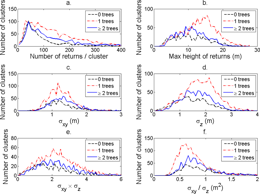
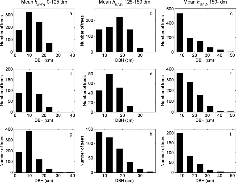
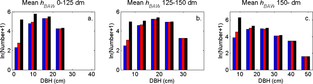
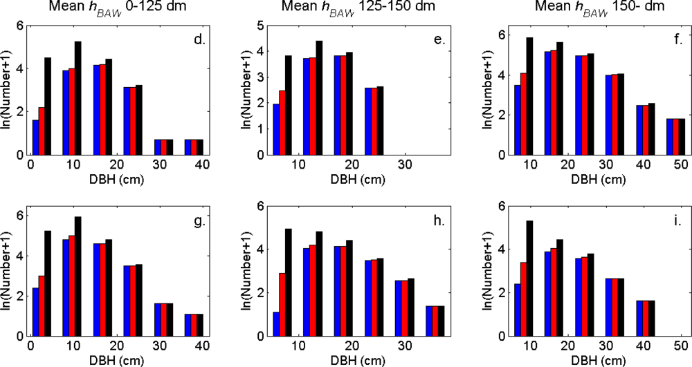
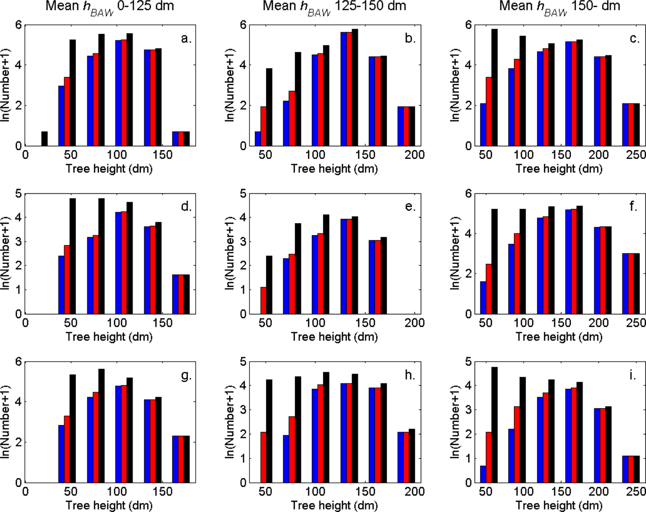
The distributions of individual features of the clusters were similar for clusters linked to zero, one and two or more trees (Figure 7). More field-measured trees below the tallest canopy layer and with a DBH < 20 cm could be linked to clusters from the tree model clustering than to segments delineated from the CS, especially in field plots with higher basal area-weighted mean tree height (Figures 8 and 9).

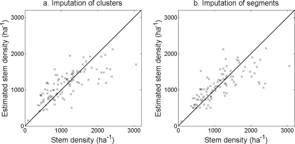
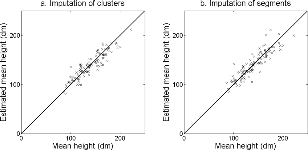
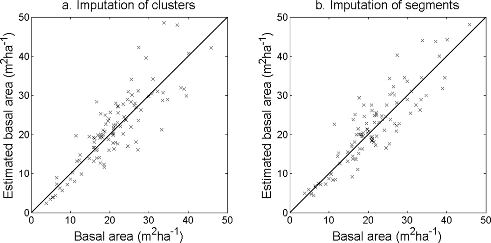
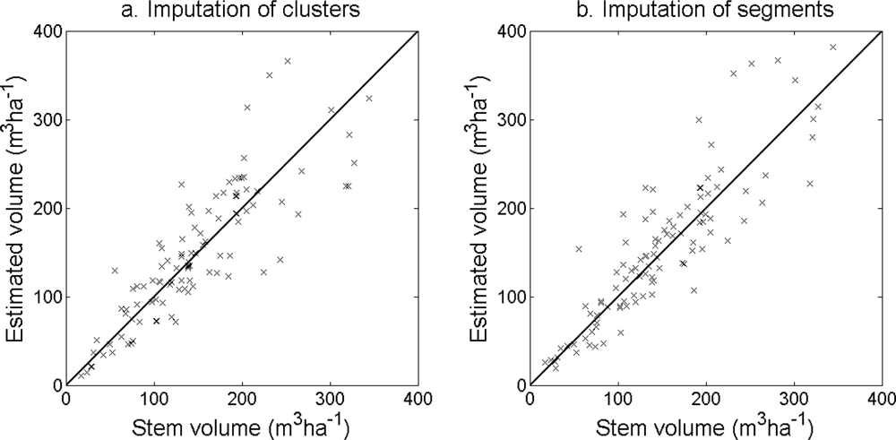
The accuracy of the estimated stem density (Figure 10) and tree height (Figure 11) was slightly higher for the imputation of clusters than for the imputation of segments (

Table 6. RMSE and bias of estimates at plot level and EI for the different models.

	Tree Model clustering, Cluster1		Tree Model Clustering, Cluster2		Segmentation, Segment1		Segmentation, Segment2
	RMSE	Bias	RMSE	Bias	RMSE	Bias	RMSE	Bias
Stem density (ha−1)	374.6 (32.7%)	5.3 (0.5%)	402.7 (35.1%)	−16.6 (−1.4%)	385.5 (33.6%)	−20.8 (−1.8%)	397.8 (34.7%)	20.8 (1.8%)
Basal area (m2·ha−1)	4.8 (22.9%)	0.4 (2.0%)	4.3 (20.3%)	0.2 (0.9%)	4.3 (20.6%)	0.5 (2.5%)	4.3 (20.2%)	0.5 (2.5%)
Stem volume (m3·ha−1)	41.9 (28.3%)	3.2 (2.1%)	38.2 (25.9%)	1.8 (1.2%)	38.6 (26.1%)	5.1 (3.5%)	38.5 (26.1%)	3.5 (2.3%)
Mean tree height (dm)	11.8 (8.4%)	−0.8 (−0.6%)	13.4 (9.5%)	−0.6 (−0.4%)	12.9 (9.2%)	0.4 (0.3%)	12.1 (8.6%)	−0.5 (−0.4%)
EI tree height	0.69		0.70		0.68		0.71
EI DBH	0.66		0.67		0.65		0.64
EI basal area	0.62		0.63		0.60		0.60

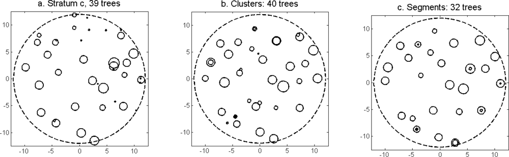
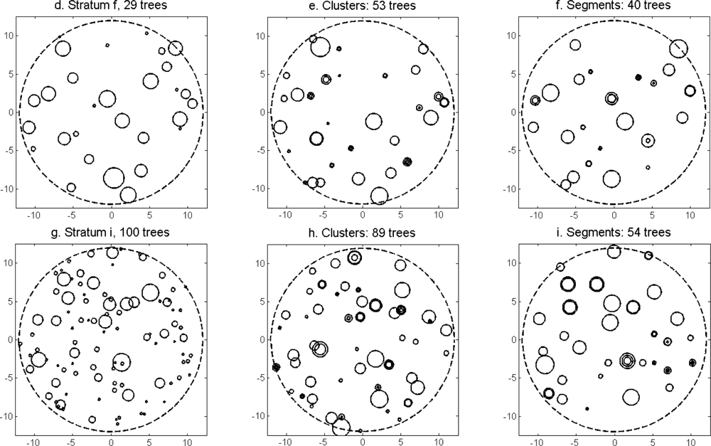
). The accuracy of the estimated basal area (Figure 12) and stem volume (Figure 13) was slightly higher for the imputation of segments than for the imputation of clusters. The EI were slightly better for the imputation of segments than for the imputation of clusters. Examples of three field plots with field-measured trees and trees imputed from clusters and segments are shown in Figure 14.

5. Discussion

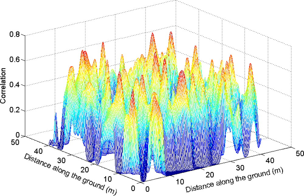
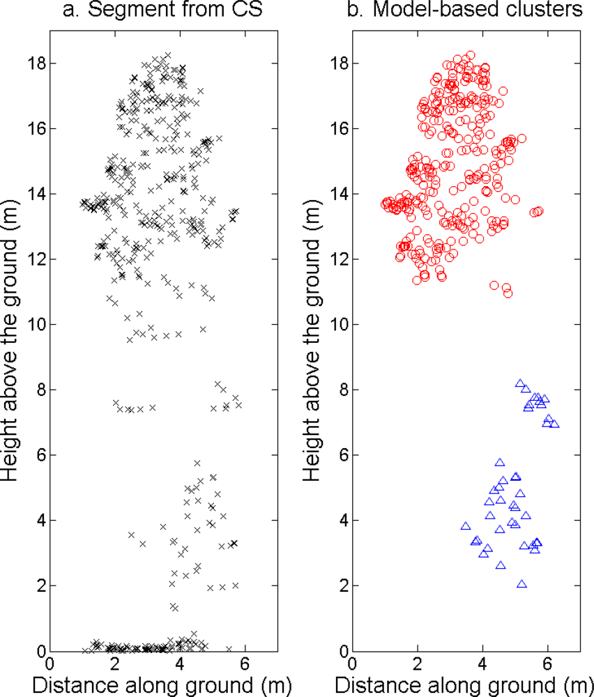
The tree crowns were delineated by segmentation of a correlation surface model followed by 3D analysis with a new tree model clustering approach. The linking of segments delineated from the CS had a high success rate for trees with a DBH ≥ 20 cm. Since the tree model clustering was based on the segmentation, the success rate was equally high in that case. However, more trees with a DBH < 20 cm could be linked to the result from the tree model clustering than to the segments delineated from the CS, especially in field plots with a higher basal area-weighted mean height where those trees were part of the understory below the tallest canopy layer. The tree model clustering appears to be successful at identifying tree crowns also for trees in the understory below the tallest canopy layer.

The accuracy at plot level of the estimated forest variables was similar for the tree model clustering and for the segmentation after k-MSN imputation. The segmentation typically identified the largest trees that contributed most to the stem volume and basal area, which resulted in accurate estimates for those forest variables. The tree model clustering divided some large tree crowns into several clusters and information was lost about those large trees. The segmentation is most successful for larger trees while methods that identify smaller trees may be less successful in delineating the tree crowns of the larger trees. The accuracy was comparable to previous studies with similar ALS data densities and forest conditions [19,20,44,45].

Tests with standard k-means clustering of the ALS returns resulted in much lower accuracy than obtained with segmentation of the CS. This was not improved by trying different parameters of the k-means clustering (e.g., different weights vertically and horizontally). For managed boreal forest, most trees can be identified successfully with segmentation of a surface model [10]. To utilize this, a tree model clustering approach was developed to combine the information derived from the CS with the 3D distribution of the ALS data below the surface model, in order to delimit the tallest tree crowns from lower vegetation and derive information about trees in the understory.

The k-means clustering divides the data into clusters based on the Euclidean distance to the cluster centres. The distances in horizontal and vertical directions had an equal weight, which means that the clusters resembled spheres. To model elongated (ellipsoid) tree crowns, different weights in horizontal and vertical directions could be used. However, tests with relative weights of 1.5–2 in the vertical direction made the result worse.

The delineation methods used in this study depend on several parameter values. Most existing methods for delineation of tree crowns from ALS data depend on parameter settings (e.g., height thresholds, raster cell sizes and filter sizes) selected manually by the operator in order to optimize the delineation [8–11,14,24,26]. Automated optimization of the parameters based on field data with known tree positions [25] could possibly be done for different forest types (e.g., coniferous forest or beech forest); however, this would require further research.

The CS was based on a priori knowledge of the shapes and proportions of tree crowns. Three-dimensional delineation of tree crowns may also benefit from using assumptions about the shapes and proportions of the tree crowns. In this study, this was achieved by fitting a parabolic surface to the top of each cluster and by joining clusters along a vertical axis if they were close enough.

The tree model clustering resulted in a large number of small clusters that could not be linked to any field-measured trees. Those un-linked clusters may correspond to parts of larger trees or to trees with a DBH smaller than the criterion to measure a tree in the field [20]. However, the result of the imputation was not impaired by the un-linked clusters, probably because the properties of the un-linked clusters differed from the linked clusters.

The segmentation method used in this study was the same as in Holmgren et al.[18] with the exception that the expected ratio of radius to model height was fixed (i.e., no training phase was used). The result of the segmentation may be improved by using a training phase to predict optimal parameter settings as a function of variables that can be derived from the ALS data. However, no training phase was used to set the parameters for the tree model clustering in this study, which means that the tree model clustering and the segmentation were based on the same conditions. The segmentation method has proved to perform well in a recent comparison with other segmentation methods for forests in Norway, Sweden, Germany, and Brazil [46].

Only parts of the laser light can pass through the higher layers of the canopy and the measurements will not cover the area completely [47]. Due to this occlusion effect, some suppressed trees will give rise to very few or no ALS returns [48]. Hence, they cannot be delineated from the ALS data and it is difficult to estimate the complete tree height distribution in such cases.

The ALS data consisted of first and last discrete returns. The last return is typically from the ground, and ALS data with intermediate returns might provide more information about the understory. Another option is to use waveform ALS data. Waveform ALS data describe the whole backscattered signal and allow for detailed processing, such as derivation of returns from the waveforms using more advanced algorithms [49] and measurements of the scattering properties of vegetation and terrain surfaces [50].

6. Conclusions

Delineation of tree crowns from a surface model based on a priori knowledge about the shape and proportion of the tree crowns identifies most of the trees in the tallest canopy layer of coniferous-dominated boreal forest and has been shown to perform at least as well as some 3D methods. Three-dimensional methods may also benefit from using a priori knowledge about the tree crowns. In this study, this was achieved with a tree model clustering approach by fitting a parabolic surface to the top of each cluster and by joining clusters along a vertical axis if they were close enough.

Segmentation of a CS (i.e., a surface model) identified 1,960 trees out of a total of 3,757, while the tree model clustering identified 2,169 trees. The results from the segmentation together with a model to estimate several trees for each delineated tree crown resulted in unbiased estimates of forest variables with a low RMSE (stem density RMSE 33.6% and bias −1.8%; stem volume RMSE 26.1% and bias 3.5%). The segmentation identified most trees with a DBH ≥ 20 cm. The tree model clustering approach was more successful than the segmentation in delineating trees with a DBH < 20 cm but did not improve the accuracy of the estimated forest variables at plot level (stem density RMSE 32.7% and bias 0.5%; stem volume RMSE 28.3% and bias 2.1%). Results from previous comparisons of segmentation of a surface model with tree crown models and clustering have shown higher accuracy for the segmentation [46,51,52]. The tree model clustering used the results from the segmentation for trees close to the top of the canopy and knowledge about the shapes and proportions of the tree crowns for all trees, which has not been done before. Three-dimensional analysis of ALS data may produce better results in forests with a large number of understory trees below the tallest canopy layer.

References

1. Kärkkäinen, L.; Matala, J.; Härkönen, K.; Kellomäki, S.; Nuutinen, T. Potential recovery of industrial wood and energy wood raw material in different cutting and climate scenarios for finland. Biomass Bioenerg 2008, 32, 934–943. [Google Scholar]
2. Söderbergh, I.; Ledermann, T. Algorithms for simulating thinning and harvesting in five european individual-tree growth simulators: A review. Comput. Electr. Agric 2003, 39, 115–140. [Google Scholar]
3. Backeus, S.; Wikström, P.; Lämås, T. A model for regional analysis of carbon sequestration and timber production. Forest Ecol. Manage 2005, 216, 28–40. [Google Scholar]
4. Wikström, P.; Edenius, L.; Elfving, B.; Eriksson, L.O.; Lämås, T.; Sonesson, J.; Öhman, K.; Wallerman, J.; Waller, C.; Klintebäck, F. The heureka forestry decision support system: An overview. Math. Comput. For. Nat. Resour. Sci 2011, 3, 87–94. [Google Scholar]
5. Maltamo, M.; Suvanto, A.; Packalén, P. Comparison of basal area and stem frequency diameter distribution modelling using airborne laser scanner data and calibration estimation. Forest Ecol. Manage 2007, 247, 26–34. [Google Scholar]
6. Næsset, E. Predicting forest stand characteristics with airborne scanning laser using a practical two-stage procedure and field data. Remote Sens. Environ 2002, 80, 88–99. [Google Scholar]
7. Packalén, P.; Maltamo, M. The k-msn method for the prediction of species-specific stand attributes using airborne laser scanning and aerial photographs. Remote Sens. Environ 2007, 109, 328–341. [Google Scholar]
8. Popescu, S.C.; Wynne, R.H. Seeing the trees in the forest: Using lidar and multispectral data fusion with local filtering and variable window size for estimating tree height. Photogramm. Eng. Remote Sensing 2004, 70, 589–604. [Google Scholar]
9. Hyyppä, J.; Kelle, O.; Lehikoinen, M.; Inkinen, M. A segmentation-based method to retrieve stem volume estimates from 3-d tree height models produced by laser scanners. IEEE Trans. Geosci. Remote Sens 2001, 39, 969–975. [Google Scholar]
10. Persson, Å.; Holmgren, J.; Söderman, U. Detecting and measuring individual trees using an airborne laser scanner. Photogramm. Eng. Remote Sensing 2002, 68, 925–932. [Google Scholar]
11. Solberg, S.; Næsset, E.; Bollandsås, O.M. Single tree segmentation using airborne laser scanner data in a structurally heterogeneous spruce forest. Photogramm. Eng. Remote Sensing 2006, 72, 1369–1378. [Google Scholar]
12. Vauhkonen, J.; Tokola, T.; Packalén, P.; Maltamo, M. Identification of scandinavian commercial species of individual trees from airborne laser scanning data using alpha shape metrics. Forest Sci 2009, 55, 37–47. [Google Scholar]
13. Holmgren, J.; Persson, Å. Identifying species of individual trees using airborne laser scanner. Remote Sens. Environ 2004, 90, 415–423. [Google Scholar]
14. Maltamo, M.; Peuhkurinen, J.; Malinen, J.; Vauhkonen, J.; Packalén, P.; Tokola, T. Predicting tree attributes and quality characteristics of scots pine using airborne laser scanning data. Silva Fenn 2009, 43, 507–521. [Google Scholar]
15. Richardson, J.J.; Moskal, L.M. Strengths and limitations of assessing forest density and spatial configuration with aerial lidar. Remote Sens. Environ 2011, 115, 2640–2651. [Google Scholar]
16. Maltamo, M.; Eerikäinen, K.; Pitkänen, J.; Hyyppä, J.; Vehmas, M. Estimation of timber volume and stem density based on scanning laser altimetry and expected tree size distribution functions. Remote Sens. Environ 2004, 90, 319–330. [Google Scholar]
17. Lindberg, E.; Holmgren, J.; Olofsson, K.; Wallerman, J.; Olsson, H. Estimation of tree lists from airborne laser scanning by combining single-tree and area-based methods. Int. J. Remote Sens 2010, 31, 1175–1192. [Google Scholar]
18. Holmgren, J.; Barth, A.; Larsson, H.; Olsson, H. Prediction of stem attributes by combining airborne laser scanning and measurements from harvesters. Silva Fenn 2012, 46, 227–239. [Google Scholar]
19. Breidenbach, J.; Næsset, E.; Lien, V.; Gobakken, T.; Solberg, S. Prediction of species specific forest inventory attributes using a nonparametric semi-individual tree crown approach based on fused airborne laser scanning and multispectral data. Remote Sens. Environ 2010, 114, 911–924. [Google Scholar]
20. Hyyppä, J.; Yu, X.; Hyyppä, H.; Vastaranta, M.; Holopainen, M.; Kukko, A.; Kaartinen, H.; Jaakkola, A.; Vaaja, M.; Koskinen, J.; et al. Advances in forest inventory using airborne laser scanning. Remote Sens 2012, 4, 1190–1207. [Google Scholar]
21. Axelsson, P.E. Processing of laser scanner data—algorithms and applications. ISPRS J. Photogramm 1999, 54, 138–147. [Google Scholar]
22. Kraus, K.; Pfeifer, N. Determination of terrain models in wooded areas with airborne laser scanner data. ISPRS J. Photogramm 1998, 53, 193–203. [Google Scholar]
23. Barilotti, A.; Sepic, F.; Abramo, E. Automatic Detection of Dominated Vegetation under Canopy Using Airborne Laser Scanning Data. Proceedings of SilviLaser 2008, 8th International Conference on LiDAR Applications in Forest Assessment and Inventory, Edinburgh, UK, 17–19 September 2008; pp. 134–143.
24. Gupta, S.; Weinacker, H.; Koch, B. Comparative analysis of clustering-based approaches for 3-D single tree detection using airborne fullwave lidar data. Remote Sens 2010, 2, 968–989. [Google Scholar]
25. Lee, H.; Slatton, K.C.; Roth, B.E.; Cropper, W.P., Jr. Adaptive clustering of airborne lidar data to segment individual tree crowns in managed pine forests. Int. J. Remote Sens 2010, 31, 117–139. [Google Scholar]
26. Morsdorf, F.; Meier, E.; Koetz, B.; Itten, K.I.; Dobbertin, M.; Allgöwer, B. Lidar-based geometric reconstruction of boreal type forest stands at single tree level for forest and wildland fire management. Remote Sens. Environ 2004, 92, 353–362. [Google Scholar]
27. Vaughn, N.R.; Moskal, L.M.; Turnblom, E.C. Tree species detection accuracies using discrete point lidar and airborne waveform lidar. Remote Sens 2012, 4, 377–403. [Google Scholar]
28. Ferraz, A.; Bretar, F.; Jacquemoud, S.; Goncalves, G.; Pereira, L.; Tome, M.; Soares, P. 3-D mapping of a multi-layered mediterranean forest using als data. Remote Sens. Environ 2012, 121, 210–223. [Google Scholar]
29. Reitberger, J.; Schnorr, C.; Krzystek, P.; Stilla, U. 3D segmentation of single trees exploiting full waveform lidar data. ISPRS J. Photogramm 2009, 64, 561–574. [Google Scholar]
30. Santoro, M.; Fransson, J.E.S.; Eriksson, L.E.B.; Magnusson, M.; Ulander, L.M.H.; Olsson, H. Signatures of alos palsar L-band backscatter in swedish forest. IEEE Trans. Geosci. Remote Sens 2009, 47, 4001–4019. [Google Scholar]
31. Lämås, T. The Haglöf Postex Ultrasound Instrument for the Positioning of Objects on Forest Sample Plots; Swedish University of Agricultural Sciences, Department of Forest Resource Management: Umeå, Sweden, 2010; p. 10. [Google Scholar]
32. The Heureka Project. Available online: http://www.slu.se/heureka (accessed on 28 September 2012).
33. Söderberg, U. Funktioner för Skogliga Produktionsprognoser. Tillväxt och Formhöjd för Enskilda Träd av Inhemska Trädslag i Sverige (in Swedish); Report 14; Institutionen för Skogstaxering (Department of Forest Survey), Swedish University of Agricultural Sciences: Umeå, Sweden, 1986. [Google Scholar]
34. Söderberg, U. Funktioner för Skogsindelning. Höjd, Formhöjd och Barktjocklek för Enskilda Träd (in Swedish); Report 52; Institutionen för Skogstaxering (Department of Forest Survey), Swedish University of Agricultural Sciences: Umeå, Sweden, 1992. [Google Scholar]
35. Elfving, B. Ålderstilldelning Till Enskilda Träd i Skogliga Tillväxtprognoser (in Swedish); Report 182; Institutionen för Skogstaxering (Department of Forest Survey), Swedish University of Agricultural Sciences: Umeå, Sweden, 2003. [Google Scholar]
36. Axelsson, P. Dem Generation from Laser Scanner Data Using Adaptive Tin Models. Proceeding of the International Archives of Photogrammetry and Remote Sensing, Amsterdam, The Netherlands, 16–22 July 2000; pp. 111–118.
37. Soininen, A. Terra Scan for Microstation, User’s Guide; Terrasolid Ltd.: Jyvaskyla, Finland, 2004; p. 132. [Google Scholar]
38. Pollock, R.J. The Automatic Recognition of Individual Trees in Aerial Images of Forests Based on a Synthetic Tree Crown Image Model; University of British Columbia: Vancouver, BC, Canada, 1996. [Google Scholar]
39. Olofsson, K.; Lindberg, E.; Holmgren, J. A Method for Linking Field-Surveyed and Aerial-Detected Single Trees Using cross Correlation of Position Images and the Optimization of Weighted Tree List Graphs. Proceedings of SilviLaser 2008, 8th International Conference on LiDAR Applications in Forest Assessment and Inventory, Heriot-Watt University, Edinburgh, UK, 17–19 September 2008; pp. 95–104.
40. MacQueen, J. Some Methods for Classification and Analysis of Multivariate Observations. Proceedings of the Fifth Berkeley Symposium on Mathematical Statistics and Probability, University of California, Berkeley, CA, USA, 21 June–18 July 1965 and 27 December 1965–7 January 1966; pp. 281–297.
41. Gonzalez, R.C.; Woods, R.E. Digital Image Processing, 3rd ed.; Pearson Prentice Hall: Upper Saddle River, NJ, USA, 2008; p. 976. [Google Scholar]
42. Moeur, M.; Stage, A.R. Most similar neighbor—An improved sampling inference procedure for natural-resource planning. Forest Sci 1995, 41, 337–359. [Google Scholar]
43. Reynolds, M.R.; Burk, T.E.; Huang, W.C. Goodness-of-fit tests and model selection procedures for diameter distribution models. Forest Sci 1988, 34, 373–399. [Google Scholar]
44. Breidenbach, J.; Nothdurft, A.; Kändler, G. Comparison of nearest neighbour approaches for small area estimation of tree species-specific forest inventory attributes in central europe using airborne laser scanner data. Eur. J. For. Res 2010, 129, 833–846. [Google Scholar]
45. Vauhkonen, J.; Korpela, I.; Maltamo, M.; Tokola, T. Imputation of single-tree attributes using airborne laser scanning-based height, intensity, and alpha shape metrics. Remote Sens. Environ 2010, 114, 1263–1276. [Google Scholar]
46. Vauhkonen, J.; Ene, L.; Gupta, S.; Heinzel, J.; Holmgren, J.; Pitkanen, J.; Solberg, S.; Wang, Y.; Weinacker, H.; Hauglin, K.M.; et al. Comparative testing of single-tree detection algorithms under different types of forest. Forestry 2012, 85, 27–40. [Google Scholar]
47. Harding, D. Pulsed Laser Altimeter Ranging Techniques and Implications for Terrain Mapping. In Topographic Laser Ranging and Scanning: Principles and Processing; Shan, J., Toth, C., Eds.; CRC Press/Taylor & Francis Group: Boca Raton, FL, USA, 2009. [Google Scholar]
48. Edson, C.; Wing, M.G. Airborne light detection and ranging (lidar) for individual tree stem location, height, and biomass measurements. Remote Sens 2011, 3, 2494–2528. [Google Scholar]
49. Persson, Å.; Söderman, U.; Töpel, J.; Ahlberg, S. Visualization and Analysis of Full-Waveform Airborne Laser Scanner Data. Proceeding of the International Archives of Photogrammetry, Remote Sensing and Spatial Information Sciences, Enschede, The Netherlands, 12–14 September 2005; pp. 103–108.
50. Wagner, W.; Hollaus, M.; Briese, C.; Ducic, V. 3D vegetation mapping using small-footprint full-waveform airborne laser scanners. Int. J. Remote Sens 2008, 29, 1433–1452. [Google Scholar]
51. Kaartinen, H.; Hyyppä, J. Eurosdr/ISPRS Project Commission II: Tree Extraction, Final Report; Official Publication No 53; EuroSDR, European Spatial Data Research: Frankfurt am Main, Germany, 2008; p. 60. [Google Scholar]
52. Kaartinen, H.; Hyyppä, J.; Yu, X.; Vastaranta, M.; Hyyppä, H.; Kukko, A.; Holopainen, M.; Heipke, C.; Hirschmugl, M.; Morsdorf, F.; et al. An international comparison of individual tree detection and extraction using airborne laser scanning. Remote Sens 2012, 4, 950–974. [Google Scholar]
Figure 1. Study area in Sweden (64°14′N, 19°50′E) and positions of the field plots.
Remotesensing 05 01932f1
Figure 2. The DBH distributions in the strata defined in Table 1.
Remotesensing 05 01932f2
Figure 3. The tree height distributions in the strata defined in Table 1.
Remotesensing 05 01932f3
Figure 4. Flow chart of the methods. The squared boxes contain data and the rounded boxes show the different parts of the methods.
Remotesensing 05 01932f4
Figure 5. Smoothed correlation surface.
Remotesensing 05 01932f5
Figure 6. Side view of ALS returns assigned to (a) one segment delineated from the CS and (b) two different clusters from the tree model clustering. ALS returns assigned to other clusters are not shown here.
Remotesensing 05 01932f6
Figure 7. (a) The distribution of number of returns/cluster. (b) Maximum height of returns. (c) Standard deviation in the horizontal plane. (d) Standard deviation in the vertical direction. (e) Product of the standard deviations. (f) Ratio of the standard deviations for clusters linked to 0, 1, and ≥2 field-measured trees.
Remotesensing 05 01932f7
Figure 8. The DBH distributions (log scale) in the strata defined in Table 1 for the segments (blue), the trees linked to clusters (red), and the field-measured trees (black).
Remotesensing 05 01932f8aRemotesensing 05 01932f8b
Figure 9. The tree height distributions (log scale) in the strata defined in Table 1 for the segments (blue), the trees linked to clusters (red), and the field-measured trees (black).
Remotesensing 05 01932f9
Figure 10. Stem density at plot level estimated from (a) imputation of clusters with model Cluster1 and (b) imputation of segments with model Segment1.
Remotesensing 05 01932f10
Figure 11. Basal area-weighted mean height at plot level estimated from (a) imputation of clusters with model Cluster1 and (b) imputation of segments with model Segment1.
Remotesensing 05 01932f11
Figure 12. Basal area at plot level estimated from (a) imputation of clusters with model Cluster1 and (b) imputation of segments with model Segment1.
Remotesensing 05 01932f12
Figure 13. Stem volume at plot level estimated from (a) imputation of clusters with model Cluster1 and (b) imputation of segments with model Segment1.
Remotesensing 05 01932f13
Figure 14. Examples of three field plots randomly selected from the strata defined in Table 1 with (a) field-measured trees in stratum c, (b) trees imputed from clusters in the same field plot, (c) trees imputed from segments in the same field plot, (d) field-measured trees in stratum f, (e) trees imputed from clusters in the same field plot, (f) trees imputed from segments in the same field plot, (g) field-measured trees in stratum i, (h) trees imputed from clusters in the same field plot, and (i) trees imputed from segments in the same field plot. The dashed lines are the borders of the 12 m radius field plots and the trees are represented by the smaller circles with diameters proportional to the DBH.
Remotesensing 05 01932f14aRemotesensing 05 01932f14b