Article

Exploring the Use of MODIS NDVI-Based Phenology Indicators for Classifying Forest General Habitat Categories

1
Institute for Environment and Sustainability, European Commission, Joint Research Centre, Via E. Fermi 2749, I-21027 Ispra (VA), Italy
2
Earth Observation Group, Centre for Ecology and Hydrology, Wallingford, OX10 8BB, UK
*
Author to whom correspondence should be addressed.
Remote Sens. 2012, 4(6), 1781-1803; https://doi.org/10.3390/rs4061781
Submission received: 20 April 2012 / Revised: 12 June 2012 / Accepted: 13 June 2012 / Published: 18 June 2012

Abstract

:
The cost effective monitoring of habitats and their biodiversity remains a challenge to date. Earth Observation (EO) has a key role to play in mapping habitat and biodiversity in general, providing tools for the systematic collection of environmental data. The recent GEO-BON European Biodiversity Observation Network project (EBONE) established a framework for an integrated biodiversity monitoring system. Underlying this framework is the idea of integrating in situ with EO and a habitat classification scheme based on General Habitat Categories (GHC), designed with an Earth Observation-perspective. Here we report on EBONE work that explored the use of NDVI-derived phenology metrics for the identification and mapping of Forest GHCs. Thirty-one phenology metrics were extracted from MODIS NDVI time series for Europe. Classifications to discriminate forest types were performed based on a Random Forests™ classifier in selected regions. Results indicate that date phenology metrics are generally more significant for forest type discrimination. The achieved class accuracies are generally not satisfactory, except for coniferous forests in homogeneous stands (77–82%). The main causes of low classification accuracies were identified as (i) the spatial resolution of the imagery (250 m) which led to mixed phenology signals; (ii) the GHC scheme classification design, which allows for parcels of heterogeneous covers, and (iii) the low number of the training samples available from field surveys. A mapping strategy integrating EO-based phenology with vegetation height information is expected to be more effective than a purely phenology-based approach.

Graphical Abstract

1. Introduction

At the 10th world Conference of the Parties to the Convention on Biological Diversity a revised and updated strategic plan for biodiversity was adopted [1]. Integral to its main objective of halting and reversing trends in biodiversity loss is the need to monitor habitats and biodiversity. In Europe, the Council, the executive body defining the general political directions and priorities of the Union, has stressed the need to integrate biodiversity concerns into all sectoral policies [2]. In this context, it is generally acknowledged that Earth Observation (EO) can provide essential tools to support national and international monitoring systems, in order to enable the continuous large scale collection of environmental data [3,4]. One of the most crucial sectors where EO can play a key role is land-cover mapping, by enabling systematic monitoring of habitats and the derivation of extent and fragmentation indicators [5].
The quality and detail achieved when mapping land cover using EO is primarily limited by the manner in which electromagnetic radiation interacts with the physical and chemical properties of the land surface. If habitat classes of interest respond similarly across the whole spectrum in terms of visible and near-infrared reflectance, thermal emission, and microwave scattering, separating these into distinct classes using EO becomes a complex problem. The BioHab habitat classification system [6] was intentionally designed with an EO-perspective on habitats, by making the nomenclature more amenable to EO’s sensitivity to vegetation physiognomy. The system is based on BioHab General Habitat Categories (GHCs) developed from the practical experience of the GB Countryside Survey [7], and adapted for continental Europe through a series of validation workshops. The GHC classification scheme is an attribute-based scheme using life forms for natural habitats and non-life forms for artificial cover. The first dichotomous divisions lead to a set of six super-categories (Urban, Cultivated, Sparsely Vegetated, Tree and Shrubs, Herbaceous wetland and other Herbaceous), which determine the series of attributes that can be used to identify the appropriate GHC. The BioHab scheme has been adopted by the European Biodiversity Observation Network project, EBONE [8], of which the main objective is to establish a framework for an integrated biodiversity monitoring and research system based on key biodiversity indicators at the European institutional level. Part of the project focused on determining the role of EO in this biodiversity monitoring system. One of the options considered was to use EO-derived habitat maps to extrapolate sample-based in situ observations. For this to work the EO derived map would have to deliver habitat classes which were, at least, thematically linked to or, at best, represent the GHC of the BioHab scheme used in situ [9]. Different approaches for delivering land cover and habitat maps from EO exist and the choice of approach often depends on the data available, e.g., [10,11]. The EBONE study reported here explored whether phenology metrics, as derived from currently available medium resolution NDVI time series, could play a role in habitat mapping and more specifically in mapping the forest (Phanerophytes) GHCs of the BioHab scheme.
The use of multi-temporal imagery has already delivered maps of natural vegetation at the biome level [12], land cover at national or regional scales [13,14], habitats [15], vegetation types [16,17], and in some cases, species [18]. Also, regular (8, 10, 16-day) time-series of EO-imagery have been exploited to derive vegetation phenology characteristics and links with climate [19] and for change analysis [20]. The methods used generally involve Principal Component Analysis [21], Fourier analysis [22], statistical analysis [23], or phenology metrics. This last approach has been used for looking at trends in growing season length in the northern hemisphere [24,25]; for separating herbaceous from woody vegetation cover [26]; for crop identification [27], or for continental estimations of biophysical parameters, such as Gross Primary Production [28].
The main objectives of the present study were twofold. First, to explore the use of MODIS NDVI-derived phenology metrics for the identification and classification of Forest GHC, and second, to provide general recommendations for the mapping of GHC types using phenology information.

2. Materials and Methods

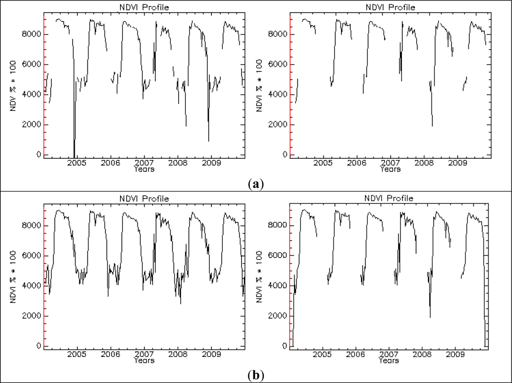
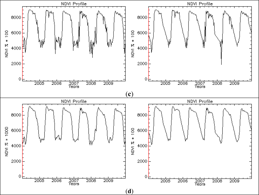
2.1. MODIS NDVI Data and Pre-Processing

A time-series of MODIS (Moderate Resolution Imaging Spectroradiometer) NDVI data was prepared. It consists of 10-day NDVI Maximum Value Composites (MVC) built according to Holben [29] from daily surface reflectance data (MOD09). The series stretches across six full years from 2004 to 2009 and covers the whole of continental Europe. The MODIS NDVI MVC series was provided to EC JRC by the Flemish Institute for Technological Research (VITO NV) and includes atmospheric correction, cloud detection, and calibration [3032]. Missing values, clouds, snow and rock outcrops were flagged. To complete the time-series, the flagged data points were substituted by their seasonal mean (i.e., mean of that 10-day period for the available years). These 10-day composites were preferred to the available MODIS 16-day composites of vegetation indices (NDVI, EVI) because their higher temporal resolution allows for more detailed and informative vegetation signal curves. Outliers were detected by applying the Chebychev’s theorem (95% confidence interval) and were also substituted by seasonal means [33]. Pixels for which no seasonal mean could be calculated, for example, pixels which are snow-covered throughout the same time periods of each year, were given a linear interpolated NDVI value using the nearest existing data points in time. Finally, NDVI data were filtered using a Savitzky-Golay smoothing filter [34], using a temporal window size of 6 decades and a polynomial function with degree m = 4. These values were found by Chen et al. [34] to represent a good trade-off between preserving temporal detail in NDVI time-series and removing potential outliers. An aggregated data gap frequency was calculated by adding up all single decadal masks (36) and combining the result with a water mask (Figure 1). This layer was used to identify regions with a high frequency of data gaps and assess the impact of data loss on our classification (Section 2.3).

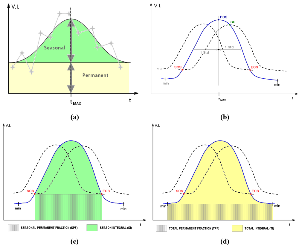
2.2. Extraction of Phenological Information

A frequent assumption in the analysis of phenology through EO-derived time series of vegetation indices (VI) is that the vegetation leaf seasonal cycles can be defined through a regular pattern [35]. An annual season cycle can be described in general terms as represented by (a) one component which is the permanent signal, or ‘background’ and (b) a variable component which is a function of seasonal dynamics [36]. The latter is generally characterized by an initial growing period, during which the VI signal increases, a maturity period when it reaches a maximum at a certain time (tMAX), and a senescence period during which the VI signal decreases back towards the background level. An idealized scheme is shown in Figure 2(a).
In reality, this pattern is influenced by a number of variables that shape and modify the VI signal: (i) the type of the vegetation contained in the remotely-sensed image pixel; (ii) the environmental variables driving the phenology (for example: precipitation, temperature, flooding, irrigation); (iii) the degree of spatial heterogeneity (e.g., land cover, vegetation type and topography) contained within the pixel; (iv) the changes in cover and condition of the vegetation over time (e.g., land cover change processes, health status, drought effects) and (v) the signal noise caused by, for example, aerosols, clouds, snow or varying solar-viewing geometry.
The regular pattern assumption described above forms the basis of the Phenolo model [37,38] used in this study, and the many other models and algorithms developed to derive phenology metrics. A lot of uncertainty still exists regarding the ‘ecological meaning’ and accuracy of phenology metrics derived from EO time-series. A comparison of a single phenology metric ‘start of season’ showed a worrying degree of variability of the metric between algorithms which for the temperate latitudes could mount up to ∼15 days in either direction [39]. Although the absolute values of the metrics may be biased and variable between approaches (including their preceding gap filling and smoothing methods), the relative differences detected using a single approach could still remain a powerful means of differentiating phenologically different vegetation types. Our choice of the Phenolo model and the preceding gap filling and smoothing method is a pragmatic one, based on ease of access and expertise in running the model.
Phenolo uses smoothing and moving average algorithms to derive a large set of phenology metrics from VI time series. A number of studies investigated vegetation dynamics by exploiting date phenology metrics [40,41], the main ones being the timing of the start and end of the growing season. To define such parameters, Phenolo (version 2009) proceeds as follows: in the first step the model applies to the VI time series a median filter on a sliding temporal window of 5 successive time points. This is followed by the calculation of one forward and one backward lagging curve using a moving average algorithm. For example, for a forward lag an x-day moving average value of time point p is calculated as the average of values for the x time points from (p-x) to p. The resulting averaged values will always reach similar magnitudes as the original p values later in time. The lag distance, defined in terms of the number of successive time points x, is defined by applying 1 standard deviation from the barycentre of the integral surface of the curve [37], as shown in Figure 2b. This value can be changed according to analyses needs.
Following Reed et al. [40], the start of the growing season (point SOS in Figure 2(b)) was defined in Phenolo as the first crossing point between the smoothed curve and the forward lagged curve. The same criterion applies for the end of season (EOS), represented by the intersection between the backward curve and the smoothed one. The point corresponding to the maximum value of the vegetation signal is the Peak of Season (POS). The Growing Season End (GE) is defined as the higher intersection point between the forward lagged curve and the signal curve. The EOS, SOS, POS and GE points define two metrics each, defined by the correspondent Day and the NDVI value on the Cartesian axes. The time interval in days between SOS and EOS defines the Season Length (SL), while the time interval between the minima in the phenology curve is referred in the model as the Total Length (ML).
By combining the above date metrics and the VI curve, the Phenolo model derives a series of productivity phenology metrics (Figure 2(c,d)). Particularly relevant among them are: (i) Seasonal Permanent Fraction (SPF), defined as the area between the line connecting Start and End of season and the x axis; (ii) the Season Integral (SI), the integral under the vegetation signal curve delimited by the start and the end of season; (iii) the Total Permanent Fraction (TPF), defined as the area between the timeline connecting the vegetation signal minima and the x-axis; (iv) and the Total Integral (TI), the integral under the vegetation signal curve delimited by the two vegetation signal minima. TI is a proxy that represents an approximation of the Net Primary Productivity [28]. The GE point defines the Growing season Integral (GI) and derived integrals (Table 1). Other phenology indicators, obtained by the model applying algebraic operations from the metrics listed above, are briefly presented in Table 1. For further discussion on phenology metrics construction in Phenolo 2009, see [37,38]. Overall, 31 metrics were extracted from the 6-year MODIS NDVI time series. The development of Phenolo is still in evolution, consequently all derived parameters’ description and their use are related to the model version that was available at the beginning of this research (ver. 2009); for this reason the calculation of certain variables is not guaranteed in future versions.

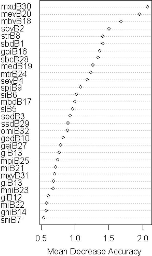
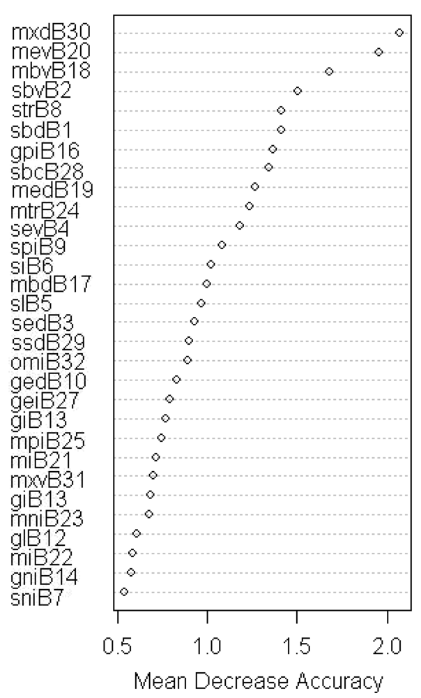
2.3. Classifications Using Random Forests

The Random Forests™ classification technique [42] was chosen to classify the extracted phenology metrics to map forest habitats as defined in the General Habitat Category scheme. Forests in this scheme are categorized as Forest Phanerophytes (FPH), within the supercategory of Shrubs and Trees (TRS). For a parcel to be given the FPH code, trees should cover at least 30% of the parcel, where a tree is defined as having a minimum height of 5 m. The following (leaf) forms allow for a further subdivision: coniferous (FPH/CON), deciduous (FPH/DEC) and evergreen (FPH/EVR) forests. Detailed information on the GHC rule-based system adopted to establish which habitat and phyto-sociological vegetation associations is represented in the Forest Phanerophytes class is described in [43].
Random Forests (RF) was chosen as it has multiple advantages: it is accurate, not sensitive to noise and computationally lighter than other classification methods. Also, this approach has been previously reported to produce promising results when applied to classify multi-source remote sensing and geographical data [44]. Breiman [42] defines Random Forests as a classifier consisting of a collection of tree structured classifiers {h(x, Θk), k=1,... } where the {Θk)} are independent identically distributed random vectors, and each tree casts a unit vote for the most popular class at input x. The collection of trees (‘forest’) classifiers finally chooses the most frequent class (mode) by combining all the ‘votes’ from the trees. Split within tree is evaluated using the Gini index, i.e., the attribute with the highest index value is chosen for the node split. Each tree is grown as follows [42]: (i) the number of cases in the training set being equal to N, then sample at random N cases with replacement; (ii) a number m<<M is specified in the way that at each node, m variables are selected at random out of the M input variables, and the best split on these m variables is used to split the node (m constant during forest growing); (iii) each tree is grown to the largest extent possible (unpruned trees). Using this bootstrap replication sampling, on average about a third of training instances (36.8%) is not used for building each tree. The M input variables are represented by the 31 phenology metrics extracted from the MODIS NDVI time series. The Random Forests needs as input a number of reference samples, which are then internally split into a set of training samples and a set of test samples. The former provides the ‘truth’ information about the classes investigated, while the latter is a set of points used to provide an estimate of error in the classification trees (‘Out Of Bag’ error, or OOB). In this classification technique, there is no need for cross-validation or a separate test to get an unbiased estimate of the error, which is internally estimated during the run [44].

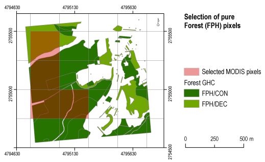
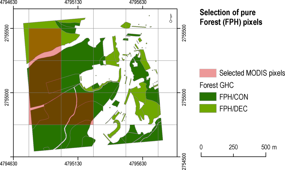
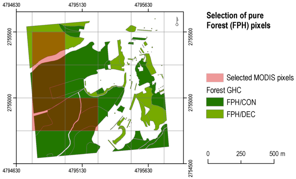
2.3.1. Field Data and Reference Pixels Selection

Reference pixels were extracted from the 1 km × 1 km field plots which were either surveyed as part of the EBONE project or sourced from existing field survey schemes of other projects. For the latter field plots, a translation of their habitat nomenclature to the GHC scheme had to be performed. A total of 99 field plots were acquired, located in Austria, Italy, south-east France and Sweden. Some of the field plots from Sweden had to be discarded from the analysis, as the NDVI time series in these regions were affected by very large periods of missing data (prolonged cloud coverage, snow, etc). The 1 km2 field plots were provided as a vector layer containing manually digitized polygons (minimum mapping unit of 0.04 ha) and their associated GHC class attributes. Polygons with Forest phanerophytes attributes (classes FPH/CON, FPH/DEC) were selected and overlaid with the 250 m grid of MODIS NDVI data (Figure 3). A pixel was considered as ‘pure’ and hence suitable as a reference pixel, if the proportion of CON or DEC was greater than or equal to 70% in the MODIS pixel. A total of 80 pure pixels was extracted (51 CON and 29 DEC). The evergreen forest type (FPH/EVR) was not evaluated due to the absence of reference data. Random Forests classifications were performed to map the coniferous and deciduous forests types, by using routines developed by Liaw and Wiener [45] in the R language. Two test regions were selected, based on the location of the reference pixels and to maximize environmental dissimilarity: (i) the territory of Austria and (ii) the Mediterranean Environmental Zone (MDN), as defined by Metzger et al. [46]. Forests in Austria are mostly coniferous, whilst the MDN zone is mainly characterized by a mixture of coniferous and deciduous.
The JRC Forest Cover Map 2006 [47] (hereafter JFM2006) was used for an independent validation of the RF classification results. JFM2006 was derived using IRS-P6 LISS-III, SPOT4 (HRVIR) and SPOT5 HRG imagery for the years 2005–2007. The overall accuracy of the JFM2006 was reported to be between 87% and 88% [48]. The spatial resolution is 25 m. The forest classes include coniferous or broad-leaved type attributes making them comparable with the GHC forest categories when the deciduous and evergreen forest classes are merged into a broad-leaf forest class. This choice was based on multiple reasons: (1) it has a pan European coverage, thus allowing inter-comparisons across a wide range of regions in Europe, (2) it covers the same period included in the MODIS NDVI time series, and (3) it is the only recent European-wide dataset holding broadleaved and coniferous forest type information. The validation dataset was produced from the JFM2006 as follows:
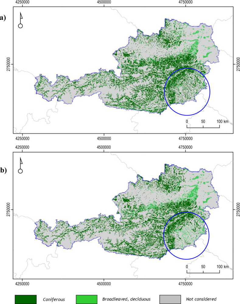
  • JFM2006 data were re-gridded to match the spatial resolution of the MODIS NDVI data by summarizing the proportion of 25 m forest pixels present within each 250 m pixel;
  • The 250 m pixels characterized by a proportion of either coniferous or broad-leaved forest ≥ 70% were selected.

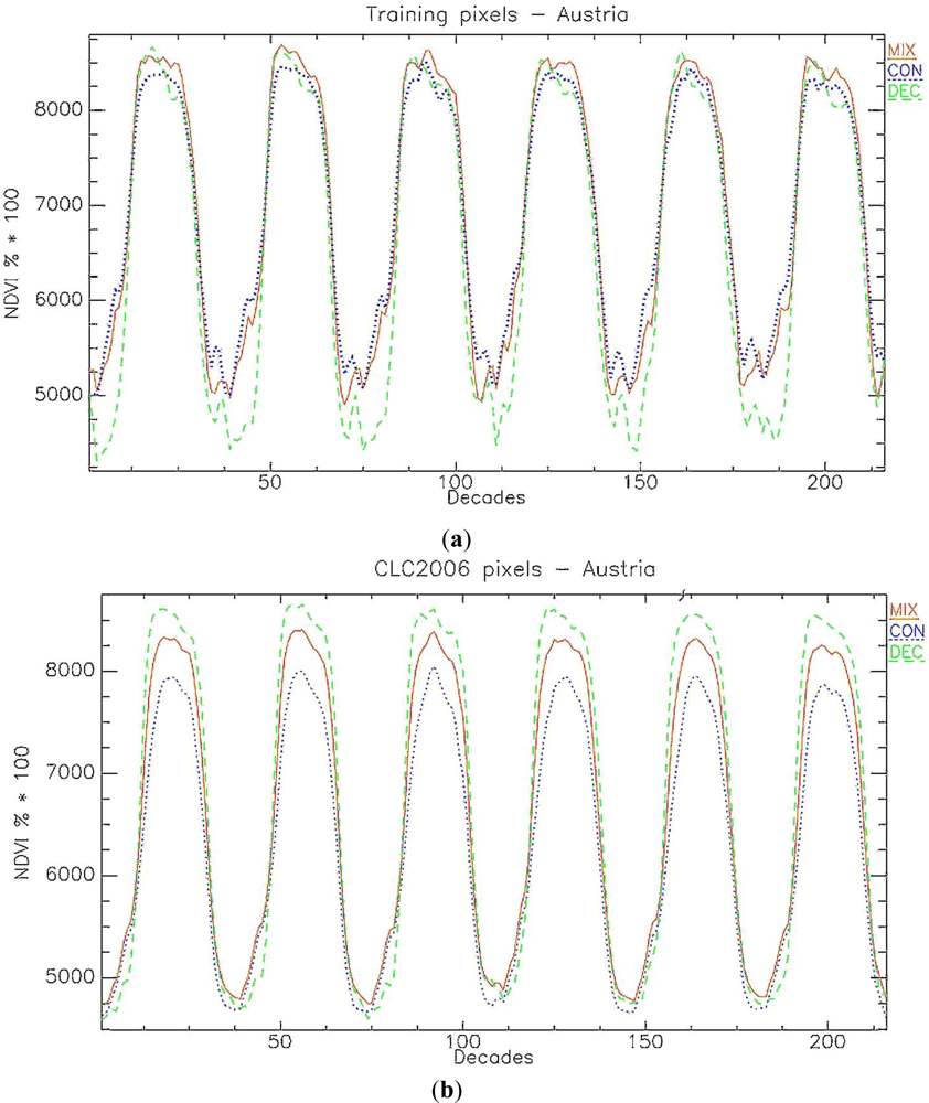
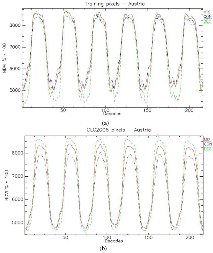
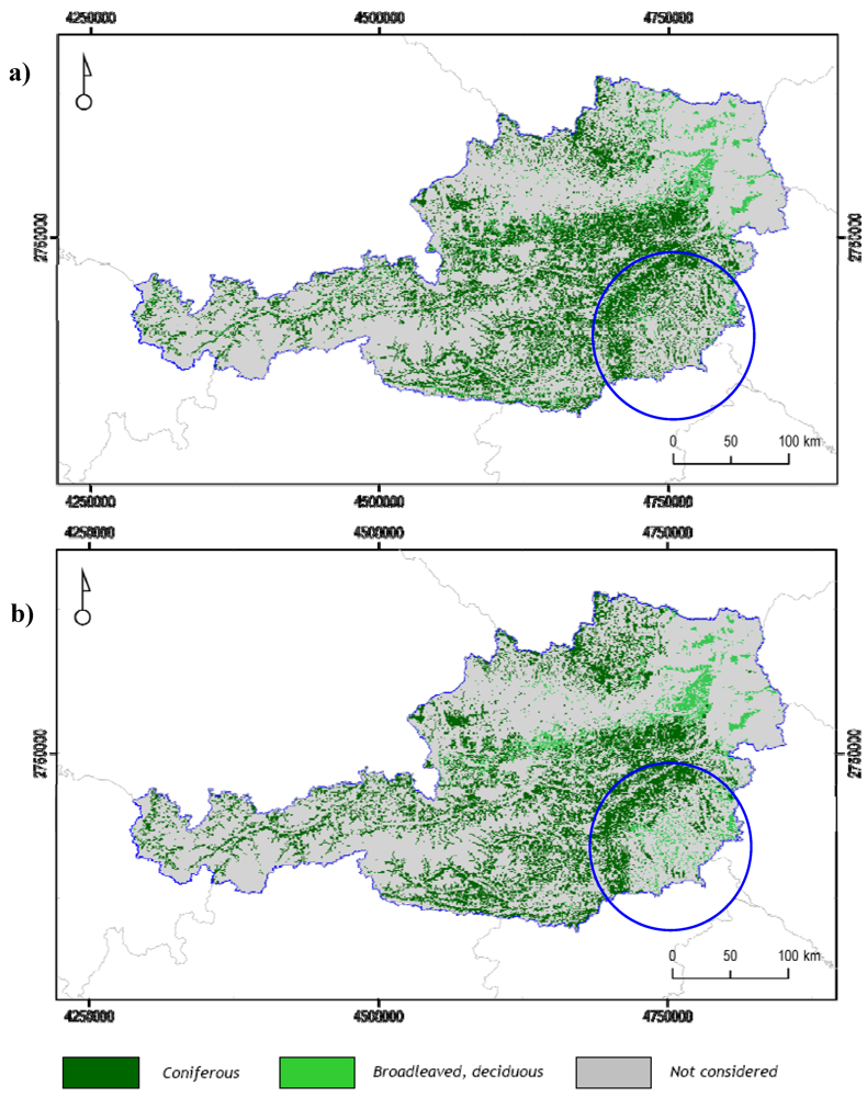
2.3.2. Classifications: Austria

To establish which of the phenology metrics are likely to contribute the most to the performance of the RF classifier, 29 recursive classification tests were performed. At every cycle the phenometric with the lowest Mean Decrease Accuracy (MDA) is excluded. MDA is a measure calculated by the RF that quantifies the decrease in classification accuracy that occurs when eliminating an input variable (i.e., a phenology indicator) from the classifier [42]; in other words, MDA is used to determine the ‘variable importance’ in the classification. For each classification the number of random phenometric used at each node (m) was set to 4, the number of trees was 500 and 100 runs were performed.
Using a sample of the reference pixels, OOB error values are calculated by the RF for each of the 29 classifications. The configurations with the two lowest OOB errors and the higher error were chosen to carry out three final RF classifications on the population of MODIS NDVI pixels that have at least 70% proportion of forest cover in the JFM2006.
The accuracy assessment was performed by carrying out a pixel based comparison between the JFM2006 validation data set and the RF forest classifications of the three phenometric configurations. For every classification, a confusion matrix is calculated to derive an overall class accuracy value. Visual observation of classification results suggested that the areas of major discordance between classified and validation data are located in regions of mixed forest formations. To investigate if the RF classification accuracy could be improved, a mixed class was introduced in the classification scheme. The mixed class is defined with the following rule: a pixel should have a proportion of FPH/CON < 70% or FPH/DEC < 70% but their sum should be greater or equal to 70% of forest (FPH). A new set of RF reference (pure) pixels representing the mixed class were identified following this rule. The phenology metrics configuration which achieved the highest overall accuracy in the previous classification exercise was selected and a RF classification performed. The JFM2006 does not provide information on mixed forest types. As a consequence, in this case an accuracy measure was derived using CORINE Land-Cover 2006 data (CLC2006) at 250 m as reference dataset (downloadable at www.eea.europa.eu), considering classes Broad-leaved forest (Class 311), Coniferous forest (Class 312) and Mixed forest (Class 313).

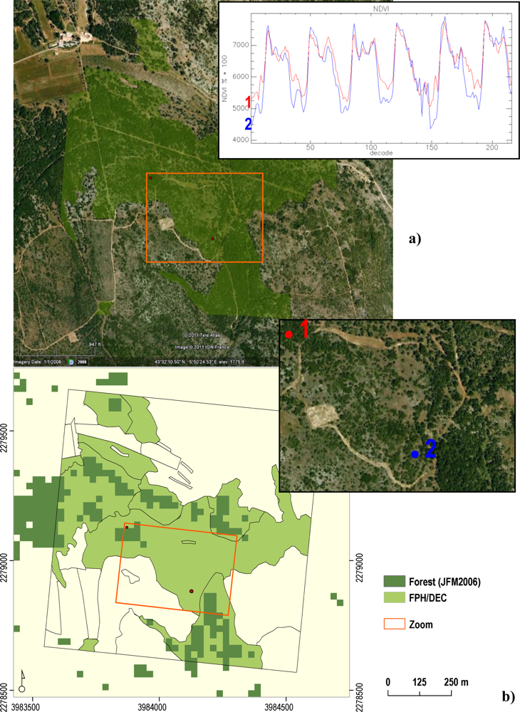
2.3.3. Classifications: Mediterranean Environmental Zone

For the Mediterranean Environmental Zone two phenology metrics configuration were chosen: (i) the one configuration which achieved the higher FPH/DEC class accuracy in the Austrian case; and (ii) the full set of metrics. RF classifications of FPH Coniferous and Deciduous forests were performed (no mixed classes), with tree numbers = 500 and m = 4. Also in this case, the subpopulation of pixels on which the classification was performed was defined by selecting the 250 m pixels that have at least a 70% share of coniferous and/or broadleaved forest calculated using the JFM2006. The accuracy assessment followed the same procedure as described for Austria. A visual inspection of the FPH/CON and FPH/DEC training pixels using GoogleEarth® was also carried out to analyze potential sources of low classification accuracy.

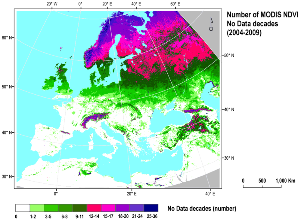
2.3.4. Classifications: The Impact of Data Gaps in VI Time Series

Time series of vegetation indices are often characterized by the presence of data gaps mainly caused by clouds, haze and snow. The potential impact of these gaps on classification accuracy was also explored. A set of NDVI pure pixels of FPH/CON and FPH/DEC showing absence of data gaps (no interpolated values in the series of NDVI MVC decades) were selected. The ‘purity’ criterion is the same as applied before. All pixels were chosen with the condition of being located within the MDN zone, and to have a correspondent pixel in the JFM2006 validation dataset. Restricting the test to the MDN zone was necessary to minimize the influence of bio-geographical variations in forest composition. The MDN zone also has a much larger proportion of gap-free time series as the incidence of cloud and snow is much lower in the southern latitudes than in the northern latitudes (Figure 1).
The following processing steps were followed:
  • Introduction of 10 consecutive data gaps (i.e., 10 contiguous no-data decades) per year across the full 6 years of MODIS NDVI time series;
  • Extraction of the FPH/CON and FPH/DEC reference (pure) pixels from the NDVI time series with added data gaps;
  • RF classifications, using all the phenology metrics, of the NDVI time series with added data gaps;
  • Accuracy assessment and comparison with classification accuracy using the original gap-free NDVI data.

3. Results and Discussion

In the classification tests performed in Austria, the Mean Decrease Accuracy parameter shows that the four most relevant variables in the RF classification are all date phenology metrics (Figure 4): day of peak of season (MXD), minimum values before SOS and after EOS (respectively MEV and MBV) and start of season value (SBV). Figure 5(a) shows a marked difference in NDVI minima values between the FPH/CON class and the FPH/DEC class in the reference data set used, explaining the RF classifier’s output. This difference in minima is also observed between ground based NDVI series collected from deciduous (broadleaved) and evergreen (coniferous and broadleaved) forests in France [49]. This study also showed marked differences in maximum values which is not so evident from our reference plots. When evaluating the time series of a different sample set, for example a random set selected from CLC2006 (Figure 5(b)), the differences in maximum NDVI values are more prominent and it is likely that the RF, using this reference set, could have identified ‘NDVI value at peak of season’ (MXV) as a relevant phenology metric.
The OOB error generally decreases when performing classifications with sets of phenology metrics listed at the top of the MDA graph. OOB errors varied from 0.092 to 0.128, showing very good accuracies for the classification of the pure pixels set. The RF classification results using the phenometric configurations that produced the two lowest (hereafter ‘A’ and ‘B’) and the highest OOB (‘C’), produced variable accuracies when compared with the JMF2006 validation data, Only the FPH/CON forest class reached good accuracy results (82%–77%), while FPH/DEC did not achieve acceptable accuracy levels: 37%–30% (Table 2).
The area with the highest discordance between the RF classifications and the JMF2006 validation dataset is located in south-east Austria in the Graz region (Figure 6). Here forest types are characterized by mixed formations, as observed in the CLC2006 map and Austrian regional maps. Despite the inclusion of the mixed forest class, the RF classification continued to produce poor accuracy results, with the exception of the FPH/CON forest class (Table 2). A study by Dokter et al. [50] showed how a gradual shift in pixel area proportion from pasture to deciduous forests was matched with a gradual shift in the EO derived date of SOS. A similar effect is to be expected for any pixels containing a mixture of covers with distinct phenological behaviors. A visual analysis of the NDVI time series of the pure pixels representing the three forest classes showed an unexpected trend in the NDVI values of the MIX forest class: in the summer period NDVI values are frequently, but only slightly, higher than both pure pixel groups representing the coniferous (FPH/CON) and deciduous (FPH/DEC) forest class. The potential for differentiation between all three classes is more towards the end of the summer, however the differences in NDVI values are very small. This behavior is not observed in a random set of CLC2006 points extracted in Austria for the same classes (Figure 5(b)), where mixed forests, as expected, show intermediate NDVI values between the two homogeneous forest classes. Also, the differences in NDVI values among the three classes are more distinct.
The two RF classifications performed in the MDN Environmental Zone also showed low classification accuracy, with values generally lower than the ones for Austria (Table 3). These results can be explained by the following three factors. Firstly, the thresholds used to select the MODIS reference pixels were based on the forest class proportion estimated from the GHCs field plot observations (Figure 3). Visual analysis of the FPH/CON and FPH/DEC training pixels, using high resolution imagery from GoogleEarth®, revealed high intra-class heterogeneity with respect to the spatial arrangement of the vegetation. As an example, polygons of FPH/DEC forest overlaid on the high resolution images showed large differences in terms of tree density and the amount of non-forest background (soil and/or understorey vegetation) present. These differences will have an impact on the pixel spectral signatures and their temporal evolution. For example, large NDVI inter-annual differences in the winter period of two FPH/DEC points within the same 1 km2 field plot are visible in Figure 7(a). In contrast, visual observation of FPH/CON forest parcels in Austria often showed dense and homogeneous forest stands. As demonstrated by Doktor et al. [50] for SOS, these variations in percentage of forest cover and background reflectance values are expected to increase the within class variability of a large number of date and productivity metrics, which could potentially decrease their effectiveness. Secondly, using validation data also derived from spectral information (JFM2006) to calculate classification accuracy is likely to lead to misleading accuracy results. This is especially true when the non-forest component is high, and forest density low (as observed in the MDN zone). Figure 7(b) shows mismatches between the JFM2006 data and the FPH/DEC field polygons. Finally, another factor which is expected to lower the classification accuracy is the absence of RF reference pixels for the FPH/EVR class (evergreen broadleaved). This was due to the small number of available GHC field plots. For a successful classification all relevant phenological classes potentially found in the area of interest should be represented by the reference data.
Our case studies suggest that the combined phenology metrics—RF approach may not be best suited for dealing with mixed/heterogeneous pixels, whether these are a mixture of forest GHCs or a mixture of forest and non-forest GHCs. Phenology metrics are designed to capture the general shape of the time-series whilst at the same time deliver measures which describe meaningful physiological events in the plant life cycle. These may not be sufficient to detect the subtle differences resulting from cover mixtures. Other approaches have been developed which could offer a solution: the use of Fourier analysis to characterize and subsequently map the full shape of a time-series of cover classes which represent a mixture of vegetated and non-vegetated attributes [22]; and temporal unmixing where a standard linear spectral unmixing procedure is applied on a pixel time-series instead of spectra [51,52]. Although the former has the advantage of being able to capture the full shape of a time-series it has the same disadvantage of our method. It requires the training for mixed classes. As mixtures represent a gradient between two or more homogeneous covers, the exact definition and identification of a mixed class is a rather ambiguous task. The latter method was tested on crop landscapes where the phenology between classes is very distinct and unlike the subtle differences we observed between FPH/DEC and FPH/CON. Without a comprehensive comparison it is not clear which of these methods would be the most effective in differentiating forest types.
The impact of data gaps in the NDVI time series on the classification results was also explored. The pre-processing applied to the NDVI time series is partly able to cope with data gaps, especially if they are short in length. For longer gaps, the latter may imply serious problems, especially if the significant phenological changes are expected to occur within the missing time gap. Statistics of NDVI decades showed that the majority of no data flags occur, as expected, in the winter period (January and December are the most affected months). This winter time interval was chosen as the more adequate to introduce the artificial no data sequences in order to simulate a real-like situation for Europe. The length of no data segments introduced is equal to 10 decades each. A comparison of the pre-processing steps carried out for a sample point using the original NDVI time series and the same with added data gaps is shown in Figure 8. Class accuracies derived from the RF classification using all phenology metrics for FPH/CON and FPH/DEC showed accuracies decreasing by only <1% for both forest types. The insertion of data gaps, contiguous and located in the same temporal windows, did not significantly change the classification outcome. Pre-processing operations dealt effectively with data gaps, producing plausible NDVI time series. This result is important in suggesting that data gaps correctly processed are not among the main factors influencing the classification performance. An analysis to test the statistical significance of change in phenology metrics from original data and with data gaps added, carried out using a random subset of 4,085 points, showed statistically significant changes. Nevertheless, these changes were not sufficient to significantly change the classification results.

4. Conclusions

The combined use of the Phenolo model with the Random Forests classification technique allowed for the extraction and classification of large sets of phenology metrics from MODIS NDVI time series for the whole of Europe in a fast and effective way. The provision by the Random Forests classifier of an unbiased internal error (Out Of Bag error) and a measure of variables importance (Mean Decrease Accuracy) helped to identify the most effective phenology metrics for forest type discrimination and classification. In the tests performed, the phenology date metrics (i.e., dates and NDVI values of specific points on the time series) were found to be more important than the productivity metrics (i.e., below time series area metrics). The most relevant Phenolo metrics were associated to the Peak of Season points (dates and NDVI values) and the curve absolute minima. Nevertheless, further analyses across a variety of landscapes and biogeographical zones are needed to infer general conclusions on the importance of single phenology metrics for forest type classification.
The Random Forest approach produced satisfactory classification accuracy in areas where pixels and field parcels are spectrally homogeneous (e.g., coniferous forest in Austria). Where these were commonly heterogeneous, the approach failed to achieve adequate mapping accuracies. The habitat classification scheme used (BioHab-General Habitat Category) is an attribute-based system, which allows for habitat parcels to consist of heterogeneous covers. In the case of the Phanerophytes class, tree cover can range from 30% to 100%. These types of classification systems are the preferred approach for continental and global land cover or habitat mapping. The result, however, is that within a parcel, heterogeneity is common and it translates into a variable set of training pixels and associated NDVI time-series. Introducing a bio-geographical zonation to reduce within attribute variability is one way forward. Creating a reference training set from homogeneous pixels that are representative of the attributes on which a classification system is another. However, the coarse size of the image pixels (250 m to 1,000 m) at which time-series are currently available do not allow for the retrieval of a sufficient number of homogeneous reference pixels required to take into account the large variability in phenology signals found across the different environmental zones. Also, when we describe heterogeneous or mixed pixels, we are referring to horizontal mixtures, whilst in this context the vertical layering of vegetation showing different phenological behaviors is as important as the horizontal one. Whilst the delivery of time series at substantially reduced pixel sizes (e.g., 10–20 m) would greatly reduce the incidence of heterogeneous pixels and so enhance the Earth Observation mapping performance, we still need to better understand (i) how spatially and temporally variable phenology signals integrate into a single signal, and (ii) how the temporal gradient of phenology changes observed in situ across species translates into the vegetation index signal. Making operational use of time series of vegetation indices to differentiate land cover or habitat types will require procedures which deliver consistent outputs across space and time. At the moment, without a comprehensive comparative assessment, it is not clear which phenology-based methods would be the most effective in differentiating forest and other habitat types.
Training and validation of Earth Observation-derived national to continental scale cover or habitat maps often suffer from a lack of suitable reference data, and our case reaffirms this issue. Earth Observation is considered to be a cost effective alternative to field-based monitoring. However, to achieve a reliable and well validated Earth Observation product, a fit-for-purpose field survey has to be an integral part of the mapping exercise. Here, the training and validation sites formed part of a field plot sampling framework designed to deliver zonal statistics on habitat extent for Europe. The option of using these field plots (10,000 across Europe) as a source of training and validation sites for Earth Observation habitat mapping requires further investigation.
In our analyses the introduction of artificial data gaps in the NDVI time series did not impact the classification accuracy and, although changes in gap configuration (e.g., number of missing data points and relative timing of the gaps) could potentially introduce more noise in the signal and eventually significantly affect the classification outcome, our results suggest that winter data gaps are not a major source of misclassification.
Finally, other habitat type elements taken into account by the BioHab-General Habitat Category (e.g., vegetation height) can provide valuable information to be considered in a classification using EO-derived information. A mapping strategy which integrates phenology metrics with, for example, vegetation height estimates from LiDAR or high resolution radar, could be potentially more effective than a pure phenology-based approach.

Acknowledgments

The authors thank S. Kay and the MARS Unit of the EC JRC for providing raw NDVI MODIS data, and E. Ivits and team (EC-JRC) for providing Phenolo software/material. Thanks are due also to P. Zuccolotto and M. Sandri (Univ. Brescia) for insightful discussions on the Random Forests classification technique. We also acknowledge the members of the EBONE project for sharing field data and for their cooperation.

References

  1. Convention on Biological Diversity (CBD). COP 10 Decisions. Proceedings of Tenth Meeting of the Conference of the Parties to the Convention on Biological Diversity, Nagoya, Japan, 18–29 October 2010.
  2. Environment Council. Conclusions of 19 December on the EU 2020 Biodiversity Strategy; 18862/11. Council of the European Union: Brussels, Belgium, 2011. Available online: http://consilium.europa.eu/media/1379139/st18862.en11.pdf (accessed on 20 March 2012).
  3. Muchoney, M.M. Earth observations for terrestrial biodiversity and ecosystems. Remote Sens. Environ 2008, 112, 1909–1911. [Google Scholar]
  4. Pereira, H.M.; Cooper, H.D. Towards the global monitoring of biodiversity change. Trends Ecol. Evol 2006, 21, 123–129. [Google Scholar]
  5. Clerici, N.; Bodini, A.; Eva, H.; Grégoire, J-M.; Dulieu, D.; Paolini, C. Increased isolation of two Biosphere Reserves and surrounding protected areas (WAP ecological complex, West Africa). J. Nat. Conserv 2007, 15, 26–40. [Google Scholar]
  6. Bunce, R.H.G.; Metzger, M.J.; Jongman, R.H.G.; Brandt, J.; de Blust, G.; Elena Rossello, R.; Groom, G.B.; Halada, L.; Hofer, G.; Howard, D.C.; et al. A Standardized Procedure for Surveillance and Monitoring European Habitats and provision of spatial data. Lands. Ecol 2008, 23, 11–25. [Google Scholar]
  7. Fuller, R.M.; Wyatt, B.K.; Barr, C.J. Countryside survey from ground and space: Different perspectives, complementary results. J. Environ. Manage 1998, 54, 101–126. [Google Scholar]
  8. Halada, L.; Jongman, R.H.G.; Gerard, F.; Whittaker, L.; Bunce, R.H.G.; Bauch, B.; Schmeller, D.S. The European Biodiversity Observation Network—EBONE. In Proceedings of the European conference of the Czech Presidency of the Council of the EU TOWARDS eENVIRONMENT Opportunities of SEIS and SISE: Integrating Environmental Knowledge in Europe; Masaryk University: Brno, Czech, 2009. [Google Scholar]
  9. Lengyel, S.; Kobler, A.; Kutnar, L.; Framstad, E.; Henry, P.-Y.; Babij, V.; Gruber, B.; Schmeller, D.; Henle, K. A review and a framework for the integration of biodiversity monitoring at the habitat level. Biodivers. Conserv 2008, 17, 3341–3356. [Google Scholar]
  10. Lucas, R.; Medcalf, K.; Brown, A.; Bunting, P.; Breyer, J.; Clewley, D.; Keyworth, S.; Blackmore, P. Updating the Phase 1 habitat map of Wales, UK, using satellite sensor data. ISPRS J. Photogramm 2011, 66, 81–102. [Google Scholar]
  11. Thomson, A.G.; Fuller, R.M.; Yates, M.G.; Brown, S.L.; Cox, R.; Wadsworth, R.A. The use of airborne remote sensing for extensive mapping of intertidal sediments and saltmarshes in eastern England. Int. J. Remote Sens 2003, 24, 2717–2737. [Google Scholar]
  12. Wessels, K.; Steenkamp, K.; von Maltitz, G.; Archibald, S. Remotely sensed vegetation phenology for describing and predicting the biomes of South Africa. Appl. Veg. Sci 2010, 14, 1–19. [Google Scholar]
  13. Fuller, R.M.; Cox, R.; Clarke, R.T.; Rothery, P.; Hill, R.A.; Smith, G.M.; Thomson, A.G.; Brown, N.J.; Howard, D.C.; Stott, A.P. The UK land cover map 2000: Planning, construction and calibration of a remotely sensed, user-oriented map of broad habitats. Int. J. Appl. Earth Obs 2005, 7, 202–216. [Google Scholar]
  14. Reese, H.M.; Lillesand, T.M.; Nagel, D.E.; Stewart, J.S.; Goldmann, R.A.; Simmons, T.E.; Chipman, J.W.; Tessar, P.A. Statewide land cover derived from multiseasonal Landsat TM data—A retrospective of the WISCLAND project. Remote Sens. Environ 2002, 82, 224–237. [Google Scholar]
  15. Dechka, J.A.; Franklin, S.E.; Watmough, M.D.; Bennett, R.P.; Ingstrup, D.W. Classification of wetland habitat and vegetation communities using multi-temporal Ikonos imagery in southern Saskatchewan. Can. J. Remote Sens 2002, 28, 679–685. [Google Scholar]
  16. Hüttich, C.; Gessner, U.; Herold, M.; Strohbach, B.J.; Schmidt, M.; Keil, M.; Dech, S. On the suitability of MODIS time series metrics to map vegetation types in dry savanna ecosystems: A case study in the Kalahari of NE Namibia. Remote Sens 2009, 1, 620–643. [Google Scholar]
  17. Van Leeuwen, W.J.; Davison, J.E.; Casady, G.M.; Marsh, S.E. Phenological characterization of desert sky island vegetation communities with remotely sensed and climate time series data. Remote Sens 2010, 2, 388–415. [Google Scholar]
  18. Hill, R.; Wilson, A.; George, M.; Hinsley, S. Mapping tree species in temperate deciduous woodland using time-series multi-spectral data. Appl. Veg. Sci 2010, 13, 86–99. [Google Scholar]
  19. Stockli, R.; Vidale, P.L. European plant phenology and climate as seen in a 20-year AVHRR land-surface parameter dataset. Int. J. Remote Sens 2004, 25, 3303–3330. [Google Scholar]
  20. McCloy, K.R. Development and evaluation of phenological change indices derived from time series of image data. Remote Sens 2010, 2, 2442–2473. [Google Scholar]
  21. Townshend, J.R.G.; Goff, T.E.; Tucker, C.J. Multitemporal dimensionality of images of normalized difference vegetation index at continental scales. IEEE Trans. Geosci. Remote Sens 1985, 23, 888–895. [Google Scholar]
  22. Geerken, R.; Zaitchik, B.; Evans, J.P. Classifying rangeland vegetation type and coverage from NDVI time-series using Fourier Filtered Cycle Similarity. Int. J. Remote Sens 2005, 26, 5535–5554. [Google Scholar]
  23. Verstraete, M.M.; Gobron, N.; Aussedat, O.; Robustelli, M.; Pinty, B.; Widlowski, J.-L.; Taberner, M. An automatic procedure to identify key vegetation phenology events using the JRC-FAPAR Products. Adv. Space Res 2008, 41, 1773–1783. [Google Scholar]
  24. Myneni, R.B.; Keeling, C.D.; Tucker, C.J.; Asrar, G.; Nemani, R.R. Increased plant growth in the northern high latitudes from 1981 to 1991. Nature 1997, 386, 698–702. [Google Scholar]
  25. Bradley, B.A.; Mustard, J.F. Comparison of phenology trends by land cover class: a case study in the Great Basin, USA. Glob. Change Biol 2008, 14, 334–346. [Google Scholar]
  26. Lu, H.; Raupach, M.R.; McVicar, T.R.; Barrett, D.J. Decomposition of vegetation cover into woody and herbaceous components using AVHRR NDVI time series. Remote Sens. Environ 2003, 86, 1–18. [Google Scholar]
  27. Jakubauskas, M.; Legates, D.; Kastens, J. Crop identification using harmonic analysis of time series AVHRR NDVI data. Comput. Electron. Agr 2002, 37, 127–139. [Google Scholar]
  28. Jung, M.; Verstraete, M.; Gobron, N.; Reichstein, M.; Papale, D.; Bondeau, A.; Robustelli, M.; Pinty, B. Diagnostic assessment of European gross primary production. Glob. Change Biol 2008, 14, 2349–2364. [Google Scholar]
  29. Holben, B.N. Characteristics of maximum-value composite images from temporal AVHRR data. Int. J. Remote Sens 1986, 7, 1417–1437. [Google Scholar]
  30. Rahman, H.; Dedieu, G. SMAC: A simplified method for the atmospheric correction of satellite measurements in the solar spectrum. Int. J. Remote Sens 1994, 15, 123–143. [Google Scholar]
  31. Paola, J.D.; Schowengerdt, R.A. A review and analysis of Backpropagation neural networks for classification of remotely sensed multispectral imagery. Int. J. Remote Sens 1995, 16, 3033–3058. [Google Scholar]
  32. Klisch, A.; Royer, A.; Lazar, C.; Baruth, B.; Genovese, G. Extraction of phenological parameters from temporally smoothed vegetation indices. Int. Arch. Photogramm. Remote Sens. Spat. Inf. Sci 2005, 36, 91–96. [Google Scholar]
  33. Lohninger, H. Teach/Me Data Analysis; Springer-Verlag: Berlin, Germany, 1999. [Google Scholar]
  34. Chen, J.; Jönsson, P.; Tamura, M.; Gu, Z.; Matsushita, B.; Eklundh, L. A simple method for reconstructing a high-quality NDVI time-series data set based on the Savitzky–Golay filter. Remote Sens. Environ 2004, 91, 332–344. [Google Scholar]
  35. Jönsson, P.; Eklundh, L. TIMESAT—A program for analysing time-series of satellite sensor data. Comput. Geosci 2004, 30, 833–845. [Google Scholar]
  36. Weissteiner, C.; Sommer, S.; Strobl, P. Time Series Analysis of NOAA AVHRR Green Vegetation Fraction as a Means to Derive Permanent and Seasonal Vegetation Component. Proceedings from the EARSeL Workshops in the Framework of the 27th Symposium, Bozen, Italy, 7–9 June 2007.
  37. Ivits, E.; Cherlet, M.; Mehl, W.; Sommer, S. Estimating the ecological status and change of riparian zones in Andalusia assessed by multi-temporal AVHHR datasets. Ecol. Indic 2009, 9, 422–431. [Google Scholar]
  38. Ivits, E.; Cherlet, M.; Mehl, W.; Sommer, S. Spatial Assesment of the Status of Riparian Zones and Related Effectiveness of Agri-Environmental Schemes in Andalusia, Spain; EUR Report; EUR 23299 N1018-5593; JRC: Luxembourg, 2008. [Google Scholar]
  39. White, M.A.; De Beurs, K.M.; Didan, K.; Inouye, D.W.; Richardson, A.D.; Jensenk, O.P.; O’Keefe, J.; Zhang, G.; Nemani, R.R.; Van Leeuwen, W.J.D.; Brown, J.F.; et al. Intercomparison, interpretation, and assessment of spring phenology in North America estimated from remote sensing for 1982–2006. Glob. Change Biol 2009, 15, 2335–2359. [Google Scholar]
  40. Reed, B.C.; Brown, J.F.; Vander Zee, D.; Loveland, T.R.; Merchant, J.W.; Ohlen, D.O. Measuring phenological variability from satellite imagery. J. Veg. Sci 1994, 5, 703–714. [Google Scholar]
  41. Hill, M.J.; Donald, G.E. Estimating spatio-temporal patterns of agricultural productivity in fragmented landscapes using AVHRR NDVI time series. Remote Sens. Environ 2003, 84, 367–384. [Google Scholar]
  42. Breiman, L. Random Forests. Mach. Learn 2001, 45, 5–32. [Google Scholar]
  43. Bunce, R.G.H.; Roche, P.; Bogers, M.M.B.; Walczak, M.; de Blust, G.; Geijzendorffer, I.R.; Van den Borre, J.; Jongman, R.H.G. Handbook for Surveillance and Monitoring of Habitats, Vegetation and Selected Species; EBONE Deliverable Report. Alterra: Wageningen, The Netherlands, 2010. Available online: http://www.ebone.wur.nl/UK/Publications/Deliverables/ (accessed on 1 February 2012).
  44. Gislason, P.O.; Benediktsson, J.A.; Sveinsson, J.R. Random Forests for land cover classification. Pattern Recogn. Lett 2004, 27, 294–300. [Google Scholar]
  45. Liaw, A.; Wiener, M. Classification and regression by RandomForests. R News 2002, 2, 18–22. [Google Scholar]
  46. Metzger, M.J.; Bunce, R.G.H.; Jongman, R.H.G.; Mücher, C.A.; Watkins, J.W. A climatic stratification of the environment of Europe. Glob. Ecol. Biogeogr 2005, 14, 549–563. [Google Scholar]
  47. Kempeneers, P.; Sedano, F.; Seebach, L.; Strobl, P.; San-Miguel-Ayanz, J. Data fusion of different spatial resolution remote sensing images applied to forest-type mapping. IEEE Trans. Geosci. Remote Sens 2011, 99, 1–10. [Google Scholar]
  48. Kempeneers, P.; Sedano, F.; Seebach, L.; San-Miguel-Ayanz, J. A High Resolution PAN-European Forest Type Map Based on Multispectral and Multi-Temporal Remote Sensing Data. Proceedings of ForestSat2010 Conference: Operational Tools in Forestry Using Remote Sensing Techniques, Lugo and Santiago de Compostela. Spain, 7–10 Semptember 2010.
  49. Soudani, K.; Hmimina, G; Delpierre, N.; Pontailler, J.Y.; Aubinet, M.; Bonal, D.; Caquet, B.; de Grandcourt, A.; Burban, B.; Flechard, C.; et al. Ground-based Network of NDVI measurements for tracking temporal dynamics of canopy structure and vegetation phenology in different biomes. Remote Sens. Environ 2012, 123, 234–245. [Google Scholar]
  50. Doktor, D.; Bondeau, A.; Koslowski, D.; Badeck, F.W. Influence of heterogeneous landscapes on computed green-up dates based on daily AVHRR NDVI observations. Remote Sens. Environ 2009, 113, 2618–2632. [Google Scholar]
  51. Lobell, D.B.; Asner, G.P. Cropland distributions from temporal unmixing of MODIS data. Remote Sens. Environ 2004, 93, 412–422. [Google Scholar]
  52. Benhadj, I.; Duchemin, B.; Maisongrande, P.; Simonneaux, V.; Khabba, S.; Chehbouni, A. Automatic unmixing of MODIS multitemporal data for inter-annual monitoring of land use at a regional scale (Tensift, Morocco). Int. J. Remote Sens 2012, 33, 1325–1348. [Google Scholar]
Figure 1. Frequency of decadal (i.e., 10 day) data gaps in MODIS NDVI across Europe caused by missing values, cloud, snow and rock outcrops showing a gradual increase in data gap frequency with latitude and problem areas in the mountains.
Remotesensing 04 01781f1
Figure 2. Observed VI values (grey crosses) and seasonal/permanent components of a theoretical vegetation cycle, modified from [24] (a). Smoothed curve (blue) and forward and backward lagging curves (dotted) defining phenology metrics in Phenolo v.2009 [37] (b). Examples of Phenolo productivity phenology metrics (c,d).
Remotesensing 04 01781f2
Figure 3. Forest phanerophytes polygons identified in the field plot, FPH/CON (dark green) and FPH/DEC (light green), are overlaid with the MODIS NDVI grid (250 m) to extract the reference pixels (in transparent red). LAEA projection.
Remotesensing 04 01781f3
Figure 4. Mean Decrease Accuracy values from the first iterative RF classification (FPH/CON, FPH/DEC) using all phenology metrics (Austria).
Remotesensing 04 01781f4
Figure 5. Average NDVI time series for pure 250m MODIS pixels in Austria of FPH/CON, FPH/DEC and MIX classes identified through (a) the GHC forest reference set of 1 km2 field plots in Austria; (b) a random set extracted from the CLC2006 map.
Remotesensing 04 01781f5
Figure 6. Maps of (a) Random Forest classification with best accuracy values; (b) forest layer derived from the JRC Forest Cover Map 2006 (LAEA projection). The blue circles indicate the area of major disagreement.
Remotesensing 04 01781f6
Figure 7. FPH/DEC polygons (transparent green) (a) over GoogleEarth® images, with NDVI trends of two pure pixels. (b) FPH/DEC over JFM2006 data at 25 m (dark green).
Remotesensing 04 01781f7
Figure 8. Pre-processing chain applied to the NDVI time series of a 250 m pixel representing a deciduous broadleaved forest (FPH/DEC): the original time series (left column) and the time series with added data gaps (right). Original NDVI data (a); substitution with seasonal means and outlier analysis (b); interpolated no data values between nearest existing points in time (c); Savitzky-Golay filtering (d).
Remotesensing 04 01781f8aRemotesensing 04 01781f8b
Table 1. Phenology metrics extracted by Phenolo (ver. 2009), with short explanation and acronyms defined in the model.
Phenology IndicatorAcronym in Phenolo
Start of Season, SOS (Day)SBD
Start of Season, SOS (Value)SBV
End of Season, EOS (Day)SED
End of Season, EOS (Value)SEV
Season Length (EOS-SOS)SL
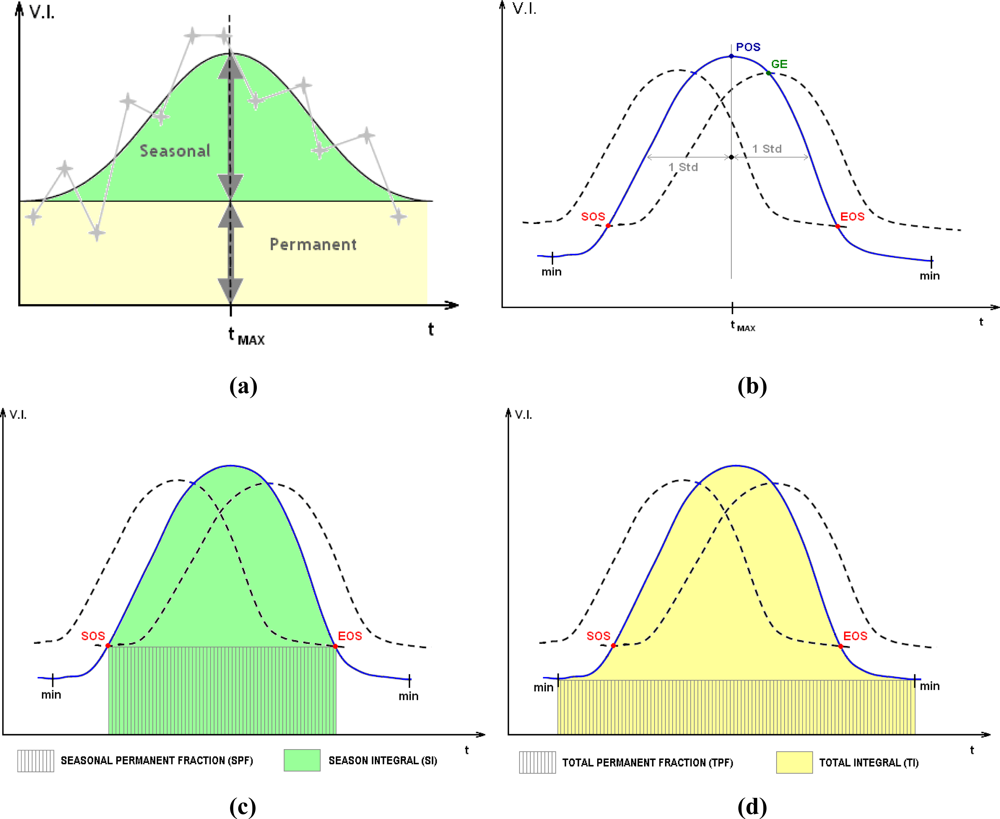
Season Integral: the integral under the vegetation signal curve delimited by EOS and SOSSI
Normalized Season IntegralSNI
Seasonal Permanent Fraction: the area below the line connecting SOS with EOS, and the x axis.SPI
Season Total Ratio [SI/(SI+SPF)]STR
Growing Season End, GE (day)GED
Growing Season End, GE (value)GEV
Growing Season LengthGL
Growing Season IntegralGI
Normalized Growing Season IntegralGNI
Growing Season Total Ratio*: [GI/(GI+SPF)]GTR
Growing Season Permanent Fraction: the permanent area fraction below the curve connecting SOS with Growing Season EndGPI
Minimum before SOS (Day)MBD
Minimum before SOS (Value)MBV
Minimum after EOS (Day)MED
Minimum after EOS (Value)MEV
Total Length: Length in time between minima (Days)ML
Total Integral, TI: the area under the vegetation signal curve delimited by the two minima.MI
Normalized Total IntegralMNI
Above Minima Total Ratio: above minima integral over TIMTR
Total Permanent Fraction, TPF: the area below the line connecting the vegetation signal minima and the x axis.MPI
Season Exceeding Integral: (TI-SI)SEI
Growing Season Exceeding Integral: (TI-GI)GEI
Season BarycentreSBC
Standard Deviation of the Season vegetation curveSSD
Peak of Season, POS (Day)MXD
Peak of Season, POS (Value)MXV
Output minus Input Length (365 – GL)OMI
*discarded.
Table 2. Class accuracies (%) in different phenology metrics configurations (Austria).
Phenology Metrics Configuration

Forest ClassABC

Coniferous – FPH/CON82.1882.3976.70
Deciduous – FPH/DEC37.3136.5529.65

Forest Class-B-

Coniferous – FPH/CON-79.03-
Deciduous – FPH/DEC-44.54-
Mixed – MIX-21.31-
Table 3. Class accuracies (%) for two phenology metrics configurations (MDN Zone).
Phenology Metrics Configuration

Forest ClassAAll
Coniferous – FPH/CON34.8447.65
Deciduous – FPH/DEC52.9658.01

