Evaluation of Broadband and Narrowband Vegetation Indices for the Identification of Archaeological Crop Marks


Abstract
:1. Introduction
2. Vegetation Indices
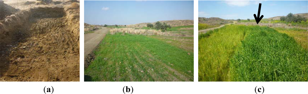
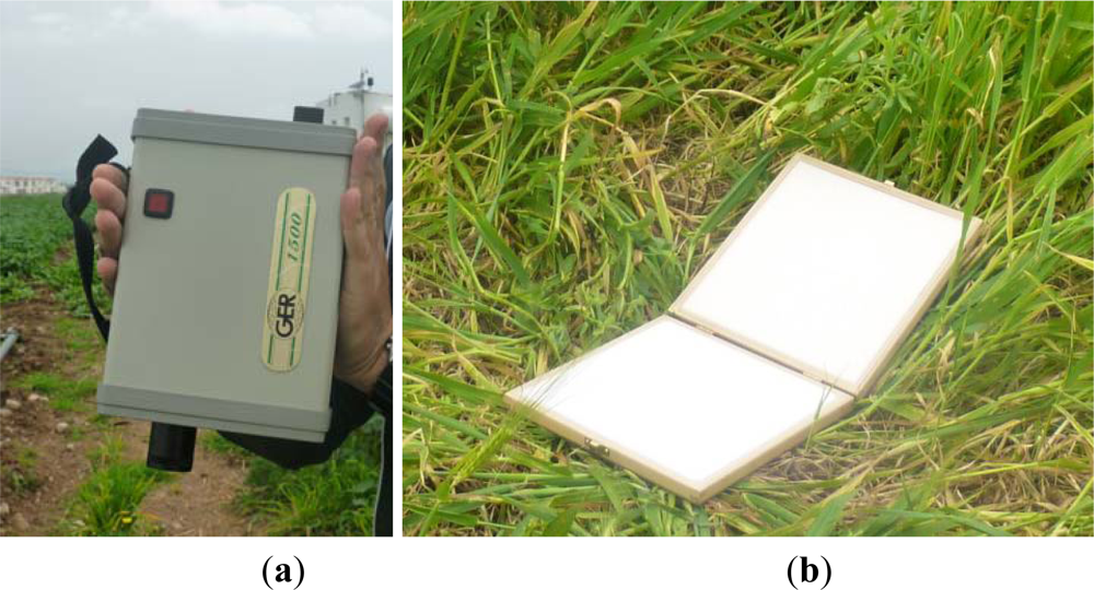
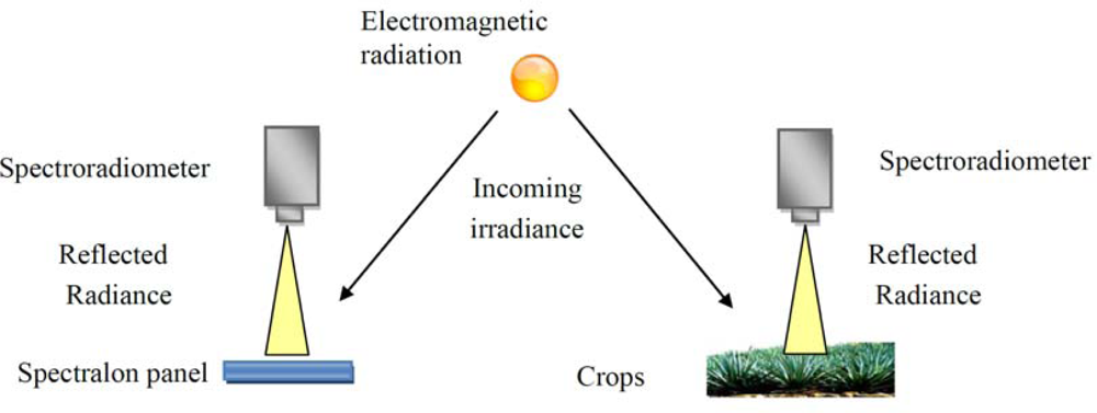
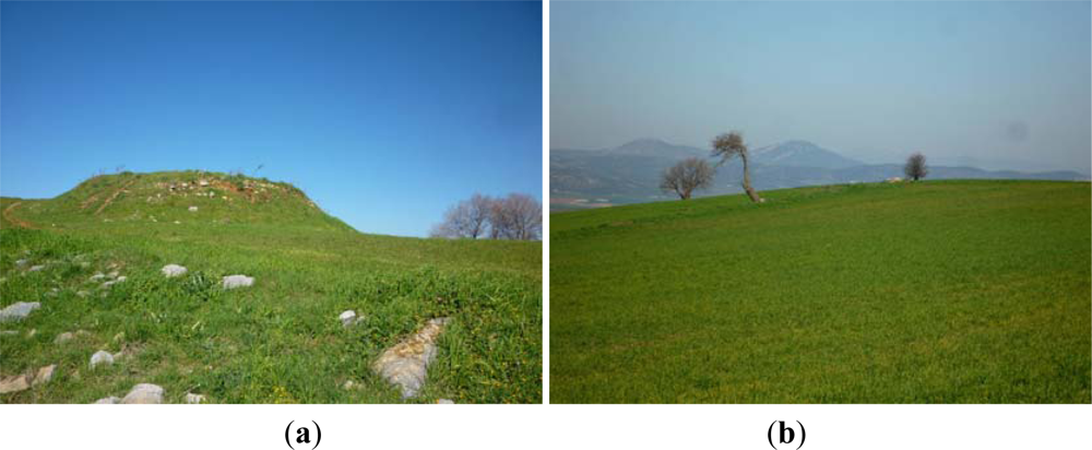
3. Case Study Area and Ground Measurements
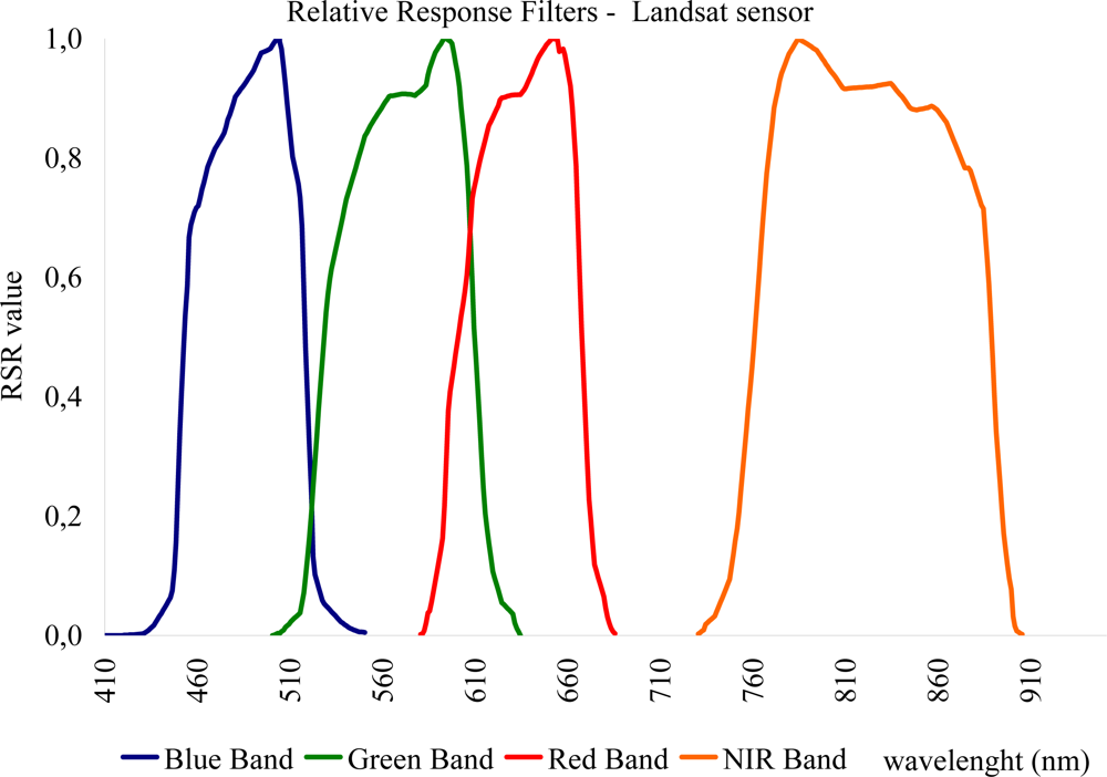
4. Methodology
- Rband = reflectance at a range of wavelength (e.g., Band 1);
- Ri = reflectance at a specific wavelength (e.g., R 450 nm);
- RSRi = Relative Response value at the specific wavelength.
5. Results
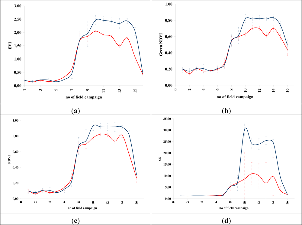
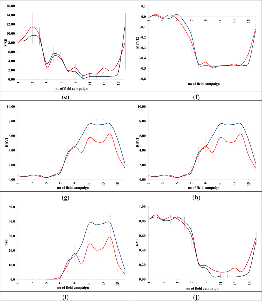
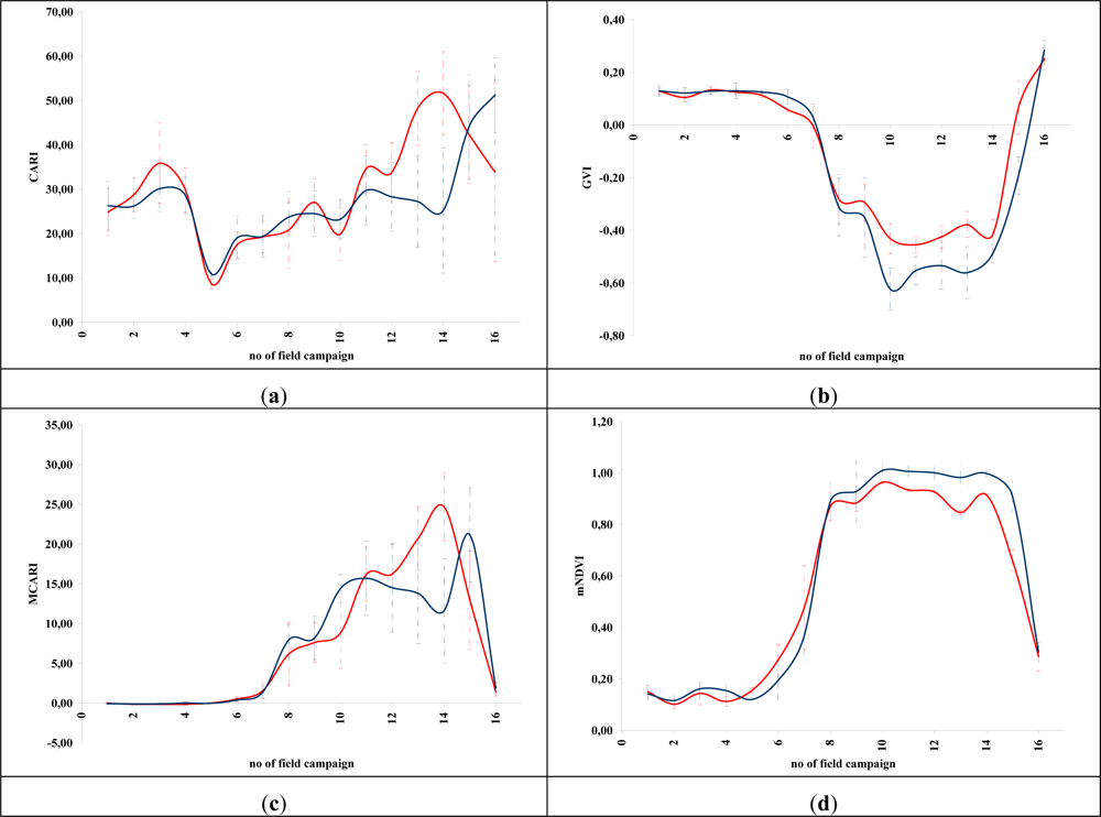
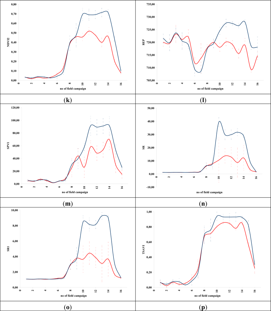
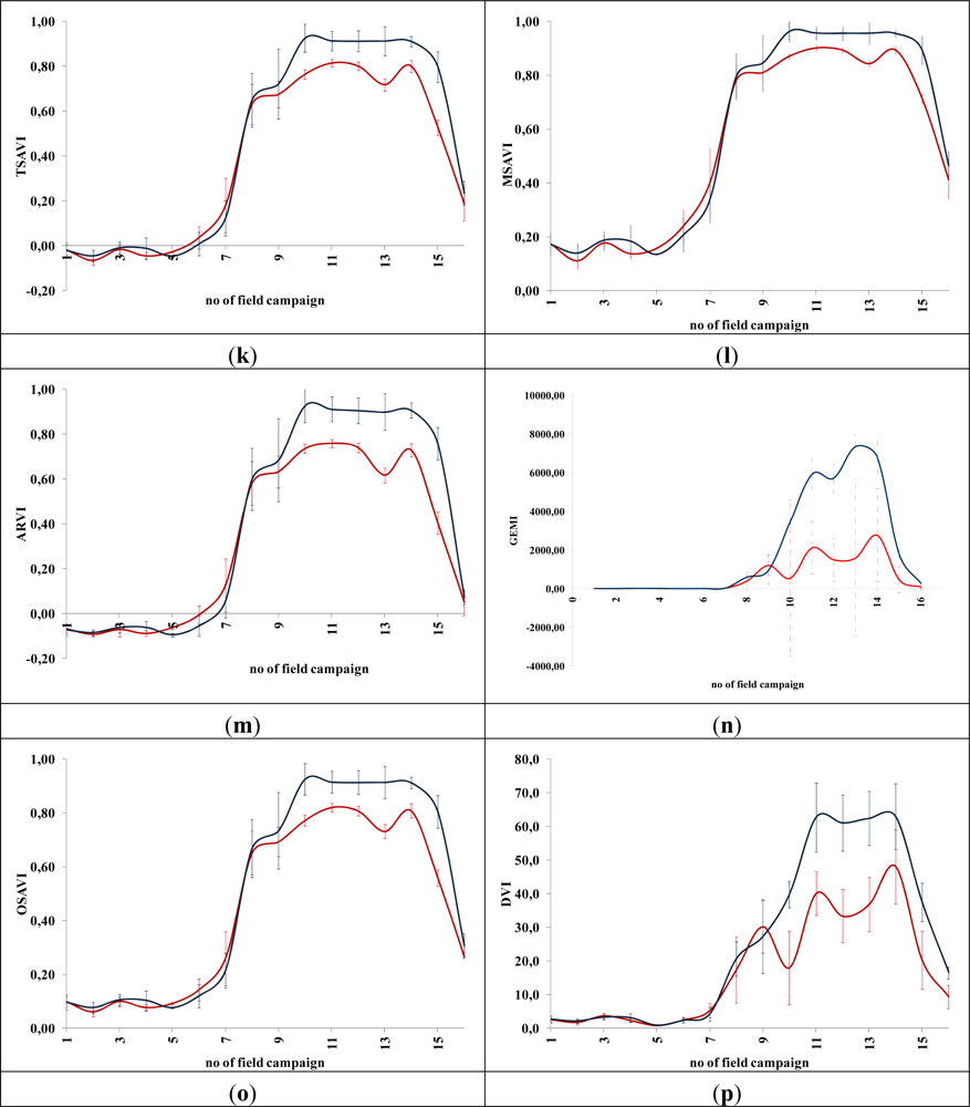
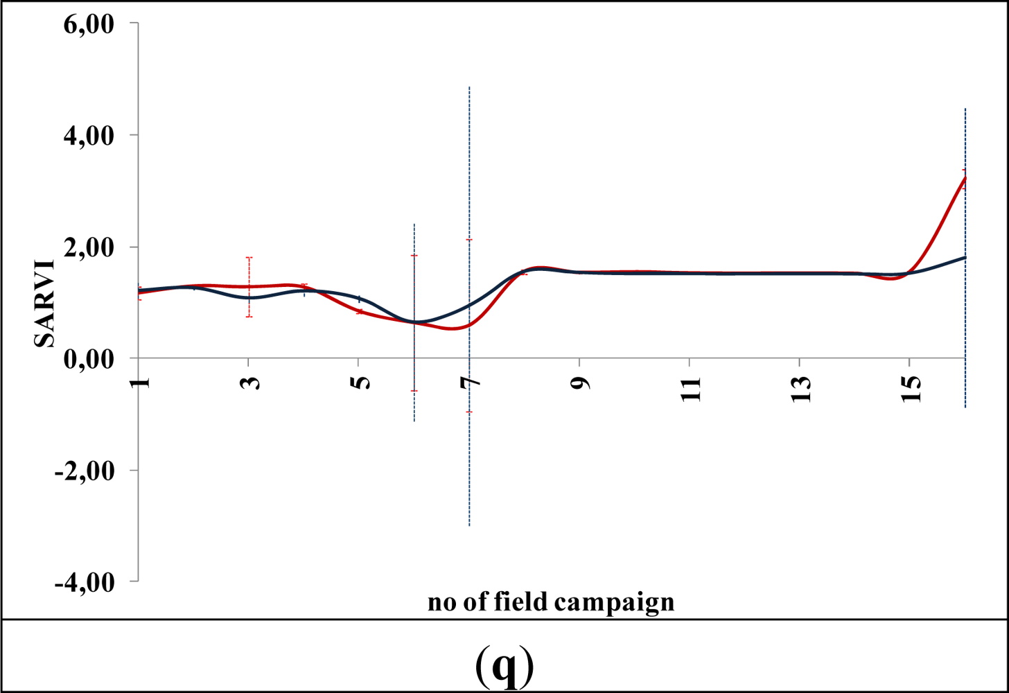
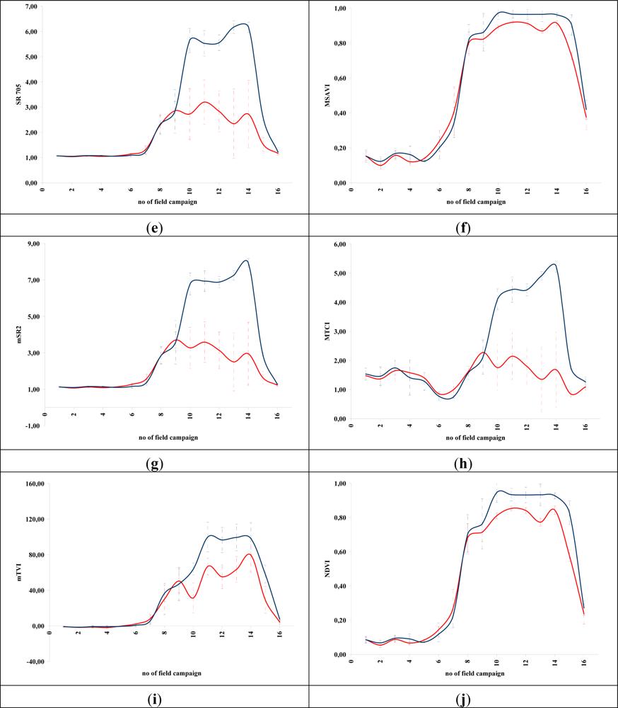
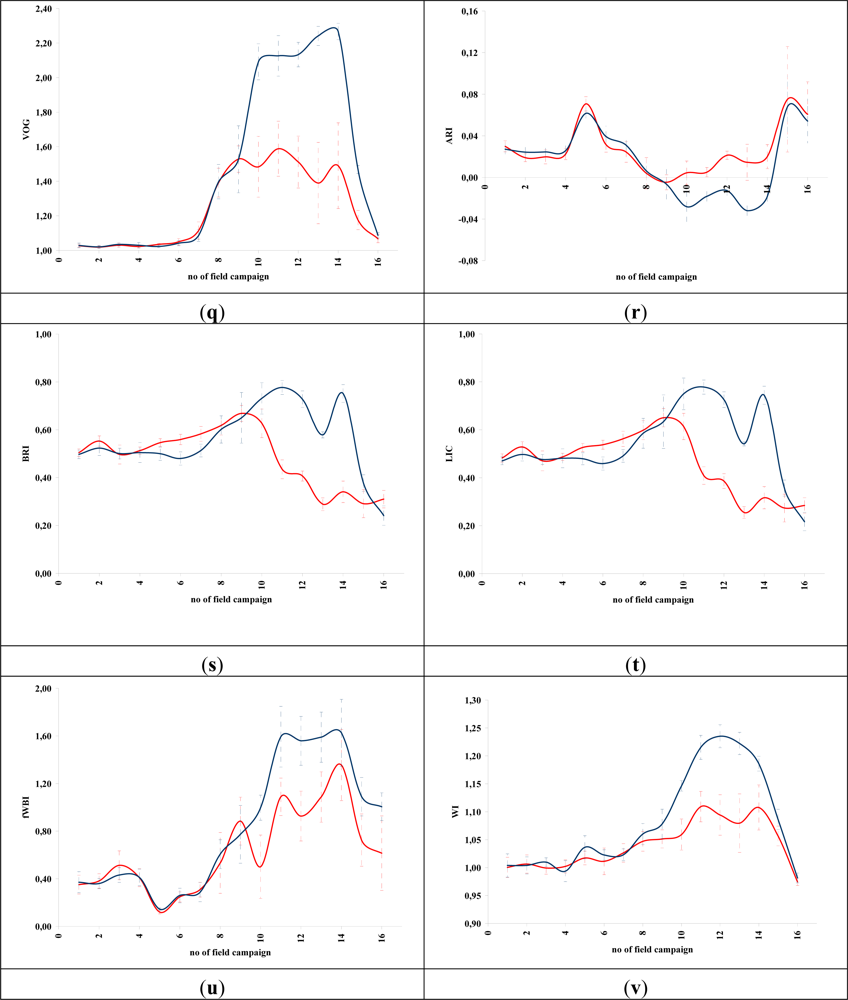
5.1. Phenological Cycle Diagrams Based on VIs
5.2. Relative Differences of VIs for the Detection of Crop Marks
- VIa.a.: the VI value over the “archaeological area”;
- max VIa.a..p.c: the maximum VI value over the “archaeological area” during the whole phenological cycle;
- VIn.a.a.: the VI value over the non “archaeological area”;
- max VIn.a.a.p.c.: is the maximum VI value over the non-archaeological area during the whole phenological cycle.
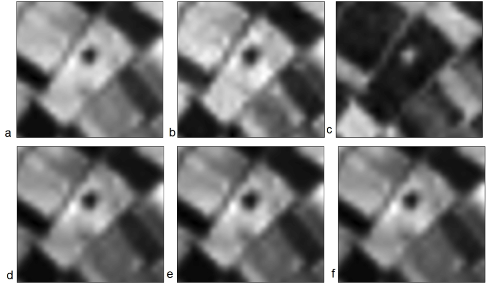
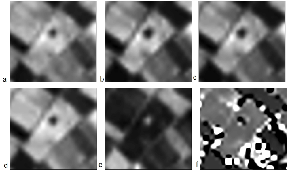
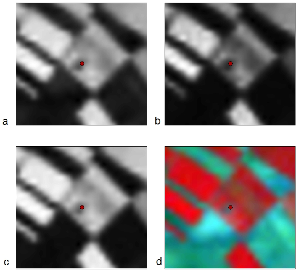
5.3. VIs Applied in Satellite Imagery for the Detection of Crop Marks
6. Conclusions
Acknowledgments
References and Notes
- Lasaponara, R.; Masini, N. Detection of archaeological crop marks by using satellite QuickBird multispectral imagerty. J. Archaeol. Sci 2007, 34, 214–221. [Google Scholar]
- Agapiou, A.; Hadjimitsis, D.G. Vegetation indices and field spectro-radiometric measurements for validation of buried architectural remains: verification under area surveyed with geophysical campaigns. J. Appl. Remote Sens 2011, 5, 05355. [Google Scholar]
- Alexakis, D.; Sarris, A.; Astaras, T.; Albanakis, K. Detection of Neolithic settlements in Thessaly (Greece) through multispectral and hyperspectral satellite imagery. Sensors 2009, 9, 1167–1187. [Google Scholar]
- de Laet, V.; Paulissen, E.; Waelkens, M. Methods for the extraction of archaeological features from very high-resolution IKONOS-2 remote sensing imagery, Hisar (southwest Turkey). J. Archaeol. Sci 2007, 34, 830–841. [Google Scholar]
- Rowlands, A.; Sarris, A. Detection of exposed and subsurface archaeological remains using multi-sensor remote sensing. J. Archaeol. Sci 2007, 34, 795–803. [Google Scholar]
- Hadjimitsis, D.G.; Themistocleous, K.; Agapiou, A.; Clayton, C.R.I. Multi-temporal study of archaeological sites in Cyprus using atmospheric corrected satellite remotely sensed data. Int. J. Architect. Comput 2009, 7, 121–138. [Google Scholar]
- Pappu, S.; Akhilesh, K.; Ravindranath, S.; Raj, U. Applications of satellite remote sensing for research and heritage management in Indian prehistory. J. Archaeol. Sci 2010, 37, 2316–2331. [Google Scholar]
- Agapiou, A.; Hadjimitsis, D.G.; Sarris, A.; Themistocleous, K.; Papadavid, G. Hyperspectral ground truth data for the detection of buried architectural remains. Lecture Notes Comput. Sci 2010, 6436, 318–331. [Google Scholar]
- Agapiou, A.; Hadjimitsis, D.G.; Alexakis, D.; Sarris, A. Observatory validation of Neolithic tells (“Magoules”) in the Thessalian plain, central Greece, using hyperspectral spectroradiometric data. J. Archaeol. Sci 2012, 39, 1499–1512. [Google Scholar]
- Aqdus, S.A.; Hanson, W.S.; Drummond, J. A Comparative Study for Finding Archaeological Crop Marks Using Airborne Hyperspectral, Multispectral and Digital Photographic Data. Proceedings of the 2007 Annual Conference of the Remote Sensing and Photogrammetry Society, Newcastle, UK, 12–17 September 2007; pp. 177–182.
- Lasaponara, R.; Masini, N. Detection of archaeological crop marks by using satellite QuickBird multispectral imagery. J. Archaeol. Sci 2007, 34, 214–221. [Google Scholar]
- Winton, H.; Horne, P. National archives for National Survey Programmes: NMP and the English Heritage Aerial Photograph Collection; Aerial Archaeology Research Group, 2010; ; Volume 2, pp. 7–18. [Google Scholar]
- White, D.C.; Williams, M.; Barr, S.L. Detecting sub-surface soil disturbance using hyperspectral first derivative band rations of associated vegetation stress. Int. Arch. Photogramm. Remote Sens. Spat. Inf. Sci. 2008, XXXVII, 243–248. [Google Scholar]
- Stagakis, S.; Markos, N.; Sykioti, O.; Kyparissis, A. Monitoring canopy biophysical and biochemical parameters in ecosystem scale using satellite hyperspectral imagery: An application on a Phlomis fruticosa Mediterranean ecosystem using multiangular CHRIS/PROBA observations. Remote Sens. Environ 2010, 114, 977–994. [Google Scholar]
- Thenkabail, S.P.; Lyon, G.J.; Huete, A. Advances in Hyperspectral Remote Sensing of Vegetation and Agricultural Croplands. In Hyperspectral Remote Sensing of Vegetation; Thenkabail, S.P., Lyon, G.J., Huete, A., Eds.; CRC Press: Boca, Raton, FL, USA, 2011; pp. 3–36. [Google Scholar]
- Thenkabail, S.P.; Lyon, G.J.; Huete, A. Hyperspectral Remote Sensing of Vegetation; CRC Press: Boca Raton, FL, USA, 2011. [Google Scholar]
- Kaimaris, D.; Georgoula, O.; Karadedos, G.; Patias, P. Aerial and Remote Sensing Archaeology in Eastern Macedonia, Greece. Proceedings of the 22nd CIPA Symposium, Kyoto, Japan, October 2009; pp. 11–15.
- Hadjimitsis, D.G.; Papadavid, G.; Agapiou, A.; Themistocleous, K.; Hadjimitsis, G.M.; Retalis, A.; Michaelides, S.; Chrysoulakis, N.; Toulios, L.; Clayton, C.R.I. Atmospheric correction for satellite remotely sensed data intended for agricultural applications: Impact on vegetation indices. Nat. Hazards Earth Syst. Sci 2010, 10, 89–95. [Google Scholar]
- Milton, E.J.; Schaepman, M.E.; Anderson, K.; Kneubühler, M.; Fox, N. Progress in field spectroscopy. Remote Sens. Environ 2009, 113, 92–109. [Google Scholar]
- Haboudane, D.; Miller, J.R.; Pattey, E.; Zarco-Tejada, P.; Strachan, I.B. Hyperspectral vegetation indices and novel algorithms for predicting green LAI of crop canopies: Modeling and validation in the context of precision agriculture. Remote Sens. Environ 2004, 90, 337–352. [Google Scholar]
- Bannari, A.; Morin, D.; Huette, A.R.; Bonn, F. A review of vegetation indices. Remote Sens. Rev 1995, 13, 95–120. [Google Scholar]
- Roberts, A.D.; Roth, L.K.; Perroy, L.R. Hyperspectral Vegetation Indices. In Hyperspectral Remote Sensing of Vegetation; Thenkabail, S.P., Lyon, G.J., Huete, A., Eds.; CRC Press: Boca Raton, FL, USA, 2011; pp. 309–328. [Google Scholar]
- Huete, A.R.; Liu, H.Q.; Batchily, K.; van Leeuwen, W. A comparison of vegetation indices over a global set of TM images for EOS-MODIS. Remote Sens. Environ 1997, 59, 440–451. [Google Scholar]
- Gitelson, A.A.; Kaufman, Y. J.; Merzlyak, M. N. Use of a green channel in remote sensing of global vegetation from EOS-MODIS. Remote Sens. Environ 1996, 58, 289–298. [Google Scholar]
- Rouse, J.W.; Haas, R.H.; Schell, J.A.; Deering, D.W.; Harlan, J.C. Monitoring the Vernal Advancements and Retrogradation (Greenwave Effect) of Nature Vegetation; NASA/GSFC Final Report; NASA: Greenbelt, MD, USA, 1974. [Google Scholar]
- Jordan, C.F. Derivation of leaf area index from quality of light on the forest floor. Ecology 1969, 50, 663–666. [Google Scholar]
- Chen, J.M. Evaluation of vegetation indices and a modified simple ratio for boreal application. Can. J. Remote Sens 1996, 22, 229–242. [Google Scholar]
- Haboudane, D.; Miller, J.R.; Pattey, E.; Zarco-Tejada, P.J.; Strachan, I. Hyperspectral vegetation indices and novel algorithms for predicting green LAI of crop canopies: modeling and validation in the context of precision agriculture. Remote Sens. Environ 2004, 90, 337–352. [Google Scholar]
- Roujean, J.L.; Breon, F.M. Estimating PAR absorbed by vegetation from bidirectional reflectance measurements. Remote Sens. Environ 1995, 51, 375–384. [Google Scholar]
- Gamon, J.A.; Surfus, J.S. Assessing leaf pigment content and activity with a reflectometer. New Phytol 1999, 143, 105–117. [Google Scholar]
- Richardson, A.J.; Wiegand, C.L. Distinguishing vegetation from soil background information. Photogram. Eng. Remote Sensing 1977, 43, 15–41. [Google Scholar]
- Pearson, R.L.; Miller, L.D. Remote Mapping of Standing Crop Biomass and Estimation of the Productivity of the Short Grass Prairie, Pawnee National Grasslands, Colorado. Proceedings of the 8th International Symposium on Remote Sensing of the Environment, Ann Arbor, MI, USA, 2–6 October 1972; pp. 1357–1381.
- Baret, F.; Guyot, G. Potentials and limits of vegetation indices for LAI and APAR assessment. Remote Sens. Environ 1991, 35, 161–173. [Google Scholar]
- Qi, J.; Chehbouni, A.; Huete, A.R.; Kerr, Y.H.; Sorooshian, S. A modified soil adjusted vegetation index. Remote Sens. Environ 1994, 48, 119–126. [Google Scholar]
- Kaufman, Y.J.; Tanré, D. Atmospherically resistant vegetation index (ARVI) for EOS-MODIS. IEEE Trans. Geosci. Remote Sens 1992, 30, 261–270. [Google Scholar]
- Pinty, B.; Verstraete, M.M. GEMI: A non-linear index to monitor global vegetation from satellites. Plant Ecol 1992, 101, 15–20. [Google Scholar]
- Rondeaux, G.; Steven, M.; Baret, F. Optimization of soil-adjusted vegetation indices. Remote Sens. Environ 1996, 55, 95–107. [Google Scholar]
- Tucker, C.J. Red and photographic infrared linear combinations for monitoring vegetation. Remote Sens. Environ 1979, 8, 127–150. [Google Scholar]
- Gong, P.; Pu, R.; Biging, G.S.; Larrieu, M.R. Estimation of forest leaf area index using vegetation indices derived from Hyperion hyperspectral data. IEEE Trans. Geosci. Remote Sens 2003, 41, 1355–1362. [Google Scholar]
- Kim, M.S.; Daughtry, C.S.T.; Chappelle, E.W.; McMurtrey, J.E., III; Walthall, C.L. The Use of High Spectral Resolution Bands for Estimating Absorbed Photosynthetically Active Radiation (APAR). Proceedings of the 6th Symposium on Physical Measurements and Signatures in Remote Sensing, Val D’Isere, France, 17–21 January 1994.
- Zarco-Tejada, P.J.; Berjón, A.; López-Lozano, R.; Miller, J.R.; Martín, P.; Cachorro, V.; González, M.R.; de Frutos, A. Assessing vineyard condition with hyperspectral indices: Leaf and canopy reflectance simulation in a row-structured discontinuous canopy. Remote Sens. Environ 2005, 99, 271–287. [Google Scholar]
- Gandia, S.; Fernández, G.; García, J.C.; Moreno, J. Retrieval of Vegetation Biophysical Variables from CHRIS/PROBA Data in the SPARC Campaing. Proceedings of the 4th ESA CHRIS PROBA Workshop, Frascati, Italy, 28–30 April 2004; pp. 40–48.
- Daughtry, C.S.T.; Walthall, C.L.; Kim, M.S.; de Colstoun, E.B.; McMurtrey, J.E. Estimating corn leaf chlorophyll concentration from leaf and canopy reflectance. Remote Sens. Environ 2000, 74, 229–239. [Google Scholar]
- Sims, D.A.; Gamon, J.A. Relationships between leaf pigment content and spectral reflectance across a wide range of species, leaf structures and developmental stages. Remote Sens. Environ 2002, 81, 337–354. [Google Scholar]
- Castro-Esau, K.L.; Sánchez-Azofeifa, G.A.; Rivard, B. Comparison of spectral indices obtained using multiple spectroradiometers. Remote Sens. Environ 2006, 103, 276–288. [Google Scholar]
- Chen, J.; Cihlar, J. Retrieving leaf area index of boreal conifer forests using Landsat Thematic Mapper. Remote Sens. Environ 1996, 55, 153–162. [Google Scholar]
- Dash, J.; Curran, P.J. The MERIS terrestrial chlorophyll index. Int. J. Remote Sens 2004, 25, 5403–5413. [Google Scholar]
- Gitelson, A.; Merzlyak, M.N. Quantitative estimation of chlorophyll-a using reflectance spectra: Experiments with autumn chestnut and maple leaves. J. Photochem. Photobiol. B: Biol 1994, 22, 247–252. [Google Scholar]
- Roujean, J.L.; Breon, F.M. Estimating PAR absorbed by vegetation from bidirectional reflectance measurements. Remote Sens. Environ 1995, 51, 375–384. [Google Scholar]
- Guyot, G.; Baret, F.; Major, D.J. High spectral resolution: Determination of spectral shifts between the red and near infrared. Int. Arch. Photogramm. Remote Sens. Spat. Inform. Sci 1988, 27, 750–760. [Google Scholar]
- Peñuelas, J.; Filella, I.; Lloret, P.; Munoz, F.; Vilajeliu, M. Reflectance assessment of mite effects on apple trees. Int. J. Remote Sens 1995, 16, 2727–2733. [Google Scholar]
- Penuelas, J.; Baret, F.; Filella, I. Semi-empirical indices to assess carotenoids/chlorophyll-a ratio from leaf spectral reflectance. Photosynthetica 1995, 31, 221–230. [Google Scholar]
- Vincini, M.; Frazzi, E.; D’Alessio, P. Angular Dependence of Maize and Sugar Beet Vis from Directional CHRIS/PROBA Data. Proceedings of the 4th ESA CHRIS PROBA Workshop, Frascati, Italy, 19–21 September 2006; pp. 19–21.
- Gitelson, A.A.; Merzlyak, M.N. Remote estimation of chlorophyll content in higher plant leaves. Int. J. Remote Sens 1997, 18, 2691–2697. [Google Scholar]
- Datt, B. Remote sensing of chlorophyll a, chlorophyll b, chlorophyll a+b, and total carotenoid content in eucalyptus leaves. Remote Sens. Environ 1998, 66, 111–121. [Google Scholar]
- Haboudane, D.; Miller, J.R.; Tremblay, N.; Zarco-Tejada, P.J.; Dextraze, L. Integrated narrow-band vegetation indices for prediction of crop chlorophyll content for application to precision agriculture. Remote Sens. Environ 2002, 81, 416–426. [Google Scholar]
- Broge, N.H.; Leblanc, E. Comparing prediction power and stability of broadband and hyperspectral vegetation indices for estimation of green leaf area index and canopy chlorophyll density. Remote Sens. Environ 2001, 76, 156–172. [Google Scholar]
- Vogelmann, J.E.; Rock, B.N.; Moss, D.M. Red edge spectral measurements from sugar maple leaves. Int. J. Remote Sens 1993, 14, 1563–1575. [Google Scholar]
- Zarco-Tejada, P.J.; Pushnik, J.C.; Dobrowski, S.; Ustin, S.L. Steady-state chlorophyll a fluorescence detection from canopy derivative reflectance and double-peak red-edge effects. Remote Sens. Environ 2003, 84, 283–294. [Google Scholar]
- Gitelson, A.A.; Merzlyak, M.N.; Chivkunova, O.B. Optical properties and nondestructive estimation of anthocyanin content in plant leaves. Photochem. Photobiol 2001, 74, 38–45. [Google Scholar]
- Zarco-Tejada, P.J.; Berjón, A.; López-Lozano, R.; Miller, J.R.; Martín, P.; Cachorro, V.; González, M.R.; de Frutos, A. Assessing vineyard condition with hyperspectral indices: Leaf and canopy reflectance simulation in a row-structured discontinuous canopy. Remote Sens. Environ 2005, 99, 271–287. [Google Scholar]
- Gitelson, A.A.; Zur, Y.; Chivkunova, O.B.; Merzlyak, M.N. Assessing carotenoid content in plant leaves with reflectance spectroscopy. Photochem. Photobiol 2002, 75, 272–281. [Google Scholar]
- Lichtenthaler, H.K.; Lang, M.; Sowinska, M.; Heisel, F.; Miehe, J.A. Detection of vegetation stress via a new high resolution fluorescence imaging system. J. Plant Physiol 1996, 148, 599–612. [Google Scholar]
- Peñuelas, J.; Gamon, J.A.; Fredeen, A.L.; Merino, J.; Field, C.B. Reflectance indices associated with physiological changes in nitrogen- and water-limited sunflower leaves. Remote Sens. Environ 1994, 48, 135–146. [Google Scholar]
- Barnes, J.D.; Balaguer, L.; Manrique, E.; Elvira, S.; Davison, A.W. A reappraisal of the use of DMSO for the extraction and determination of chlorophylls a and b in lichens and higher plants. Environ. Experimental Bot 1992, 32, 85–100. [Google Scholar]
- Gamon, J.A.; Serrano, L.; Surfus, J.S. The photochemical reflectance index: An optical indicator of photosynthetic radiation use efficiency across species, functional types, and nutrient levels. Oecologia 1997, 112, 492–501. [Google Scholar]
- Filella, I.; Amaro, T.; Araus, J.L.; Peñuelas, J. Relationship between photosynthetic radiation-use efficiency of barley canopies and the photochemical reflectance index (PRI). Physiologia Plantarum 1996, 96, 211–216. [Google Scholar]
- Merzlyak, M.N.; Gitelson, A.A.; Chivkunova, O.B.; Rakitin, V.Y. Nondestructive optical detection of pigment changes during leaf senescence and fruit ripening. Physiologia Plantarum 1999, 106, 135–141. [Google Scholar]
- Peñuelas, J.; Filella, I.; Biel, C.; Serrano, L.; Savé, R. The reflectance at the 950–970 nm region as an indicator of plant water status. Int. J. Remote Sens 1993, 14, 1887–1905. [Google Scholar]
- Agapiou, A.; Hadjimitsis, G.D.; Georgopoulos, A.; Sarris, A.; Alexakis, D.D. Towards to an archaeological index: Identify the spectral regions of stress vegetation due to buried archaeological remain. Lecture Notes Comput. Sci 2012, 7616, 129–138. [Google Scholar]
- Agapiou, A.; Hadjimitsis, G.D.; Sarris, A.; Georgopoulos, A. A New Method for the Detection of Architectural Remains Using Field Spectroscopy: Experimental Remote Sensing Archaeology. Proceedings of the XVI Congress of the UISPP, Florianopolil, Brazil, 4–10 September 2011.
- Alexakis, D.; Agapiou, A.; Hadjimitsis, D.; Sarris, A. Remote Sensing Applications in Archaeological Research. In Remote Sensing-Applications; Escalante, B, Ed.; InTech: Rijeka, Croatia, 2012; pp. 435–462. [Google Scholar]
- Wu, X.; Sullivan, T.J.; Heidinger, K.A. Operational calibration of the Advanced Very High Resolution Radiometer (AVHRR) visible and near-infrared channels. Can. J. Remote Sens 2010, 36, 602–616. [Google Scholar]
- Agapiou, A.; Hadjimitsis, G.D.; Sarris, A.; Georgopoulos, A.; Alexakis, D.D. Optimum temporal and spectral window for monitoring crop marks over archaeological remains in the Mediterranean region. J. Archaeol. Sci. 2012. 10.1016/j.jas.2012.10.036. [Google Scholar]
- Agapiou, A.; Alexakis, D.D.; Hadjimitsis, G.D. Evaluation of spectral sensitivity of ALOS, ASTER, IKONOS, LANDSAT and SPOT satellite sensors intended for the detection of archaeological crop marks. Int. J. Dig. Earth 2012. [Google Scholar] [CrossRef]
- Verhoeven, G.; Doneus, M. Balancing on the borderline—A low cost approach to visualize the red- edge shift for the benefit of the aerial archaeology. Archaeol. Prospect 2011, 18, 267–278. [Google Scholar]
- Hejcman, M.; Smrž, Z. Cropmarks in stands of cereals, legumes and winter rape indicate sub-soil archaeological features in the agricultural landscape of Central Europe. Agric. Ecosyst. Environ 2010, 138, 348–354. [Google Scholar]
- Gojda, M.; Hejcman, M. Cropmarks in main field crops enable the identification of a wide spectrum of buried features on archaeological sites in Central Europe. J. Archaeol. Sci 2012, 39, 1655–1664. [Google Scholar]
- Qi, J.; Inoue, Y.; Wiangwang, N. Hyperspectral Remote Sensing in Global Change Studies. In Hyperspectral Remote Sensing of Vegetation; Thenkabail, S.P., Lyon, G.J., Huete, A., Eds.; CRC Press: Boca Raton, FL, USA, 2011; pp. 69–90. [Google Scholar]


| No | Vegetation Index | Equation | Reference |
|---|---|---|---|
| Broadband Vegetation Indices | |||
| 1 | EVI (Enhanced Vegetation Index) | 2.5 (pNIR – pred)/(pNIR +6 pred – 7.5 pblue +1) | [23] |
| 2 | Green NDVI (Green Normalized Difference Vegetation Index) | (pNIR – pgreen)/( pNIR + pgreen) | [24] |
| 3 | NDVI (Normalized Difference Vegetation Index) | (pNIR – pred)/(pNIR + pred) | [25] |
| 4 | SR (Simple Ration) | pNIR/pred | [26] |
| 5 | MSR (Modified Simple Ratio) | pred/(pNIR/pred +1)0.5 | [27] |
| 6 | MTVI2 (Modified Triangular Vegetation Index) | [1.5(1.2*( pNIR – pgreen) – 2.5(pRed – pgreen)]/[(2 pNIR+1)2 – (6 pNIR – 5 pRed0.5) – 0.5]0.5 | [28] |
| 7 | RDVI (Renormalized Difference Vegetation Index) | (pNIR – pred)/(pNIR + pred)1/2 | [29] |
| 8 | IRG (Red Green Ratio Index) | pRed – pgreen | [30] |
| 9 | PVI (Perpendicular Vegetation Index) | (pNIR –α pred – b)/(1+α2) pNIR,soil = α pred,soil+b | [31] |
| 10 | RVI (Ratio Vegetation Index) | pred/pNIR | [32] |
| 11 | TSAVI (Transformed Soil Adjusted Vegetation Index) | [α(pNIR−α pNIR – b)]/[ (pred +α pNIR –αb+0.08(1+α2))] pNIR,soil = α pred,soil+b | [33] |
| 12 | MSAVI (Modified Soil Adjusted Vegetation Index) | [2 pNIR+1−[(2 pNIR+1)2−8(pNIR − pred)]1/2]/ 2 | [34] |
| 13 | ARVI (Atmospherically Resistant Vegetation Index) | (pNIR − prb)/( pNIR + prb), prb = pred – γ (pblue – pred) | [35] |
| 14 | GEMI (Global Environment Monitoring Index) | n(1−0.25n)( pred −0.125)/(1 − pred ) n = [2(pNIR2− pred2)+1.5 pNIR+0.5 pred]/(pNIR+ pred +0.5) | [36] |
| 15 | SARVI (Soil and Atmospherically Resistant Vegetation Index) | (1+0.5) (pNIR − prb)/( pNIR + prb +0.5) prb = pred – γ (pblue – pred) | [35] |
| 16 | OSAVI (Optimized Soil Adjusted Vegetation Index) | (pNIR – pred)/(pNIR + pred +0.16) | [37] |
| 17 | DVI (Difference Vegetation Index) | pNIR − pred | [38] |
| 18 | SR × NDVI (Simple Ratio × Normalized Difference Vegetation Index | (pNIR2 – pred)/(pNIR + pred2) | [39] |
| Narrowband Vegetation Indices | |||
| 19 | CARI (Chlorophyll Absorption Ratio Index) | p700|α670+p670+b|/[p670(α2+1)0.5 α = (p700 – p550)/150 b = p550 – 550 α | [40] |
| 20 | GI (Greenness Index) | p554/p677 | [41] |
| 21 | GVI (Greenness Vegetation Index) | (p682−p553)/(p682+p553) | [42] |
| 22 | MCARI (Modified Chlorophyll Absorption Ratio Index) | [(P700−P670)−0.2(P700−P550)](P700/P670) | [43] |
| 23 | MCARI2 (Modified Chlorophyll Absorption Ratio Index) | 1.2[2.5(p800−p670)−1.3(p800−p550)] | [28] |
| 24 | mNDVI (Modified Normalized Difference Vegetation Index) | (p800− p680)/( p800+ p680−2 p445) | [44] |
| 25 | SR705 (Simple Ratio, Estimation of chlorophyll content) | p750/ p705 | [45] |
| 26 | mNDVI2 (Modified Normalized Difference Vegetation Index) | (p750− p705)/( p750+ p705−2 p445) | [44] |
| 27 | MSAVI (Improved Soil Adjusted Vegetation Index) | [2 p800+1−[(2 p800+1)2-8(p800 – p670)]1/2]/ 2 | [34] |
| 28 | mSR (Modified Simple Ratio) | (p800−p445)/(p680−p445) | [44] |
| 29 | mSR2 (Modified Simple Ratio) | (p800−p445)/(p680−p445) | [44] |
| 30 | mSR3 (Modified Simple Ratio) | (p800/p670 − 1)/ (p800/p670 + 1)0.5 | [46] |
| 31 | MTCI (MERIS Terrestrial Chlorophyll index) | (p754−p709)/(p709−p681) | [47] |
| 32 | mTVI (modified Triangular Vegetation Index) | 1.2[1.2(p800−p550)−2.5(p670−p550)] | [28] |
| 33 | NDVI (Normalized Difference Vegetation Index) | (p800−p670)/(p800+p670) | [25] |
| 34 | NDVI2 (Normalized Difference Vegetation Index) | (p750−p705)/(p750+p705) | [48] |
| 35 | OSAVI (Optimized Soil Adjusted Vegetation Index) | 1.16(p800−p670)/(p800+p670+0.16) | [37] |
| 36 | RDVI (Renormalized Difference Vegetation Index) | (p800−p670)/(p800+p670)0.5 | [49] |
| 37 | REP(Red-Edge Position) | 700+40[(p670 + p780)/2 – p700]/(p740 – p700) | [50] |
| 38 | SIPI (Structure Insensitive Pigment Index) | (p800−p450)/(p800−p650) | [51] |
| 39 | SIPI2 (Structure Insensitive Pigment Index) | (p800−p440)/(p800−p680) | [51] |
| 40 | SIPI3(Structure Insensitive Pigment Index) | (p800−p445)/(p800−p680) | [52] |
| 41 | SPVI (Spectral polygon vegetation index) | 0.4[3.7(p800−p670)−1.2|p530−p670|] | [53] |
| Narrowband Vegetation Indices | |||
| 42 | SR (Simple Ratio) | p800/ p680 | [26] |
| 43 | SR1 (Simple Ratio) | p750/ p700 | [54] |
| 44 | SR2 (Simple Ratio) | p752/ p690 | [54] |
| 45 | SR3 (Simple Ratio) | p750/ p550 | [54] |
| 46 | SR4 (Simple Ratio) | p672/ p550 | [55] |
| 47 | TCARI (Transformed Chlorophyll Absorption Ratio Index) | 3[(p700−p670)−0.2(p700−p550)(p700/p670)] | [56] |
| 48 | TSAVI (Transformed Soil Adjusted Vegetation Index) | [α(p875−α p680 –b)]/[ (p680 +α p875 –αb+0.08(1+α2))] α = 1,062 b = 0.022 | [37] |
| 49 | TVI (Triangular Vegetation Index) | 0.5[120(p750−p550)−200(p670−p550)] | [57] |
| 50 | VOG (Vogelmann Indices) | p740/p720 | [58] |
| 51 | VOG2 (Vogelmann Indices) | (p734−p747)/(p715+p726) | [59] |
| 52 | ARI (Anthocyanin Reflectance Index ) | (1/p550)−(1/p700) | [60] |
| 53 | ARI2 (Anthocyanin Reflectance Index 2) | p800(1/p550)−(1/p700) | [60] |
| 54 | BGI (Blue Green Pigment Index) | p450/p550 | [61] |
| 55 | BRI (Blue Red Pigment Index) | p450/p690 | [61] |
| 56 | CRI (Carotenoid Reflectance Index) | (1/p510)−(1/p550) | [62] |
| 57 | RGI (Red/Green Index) | p690/p550 | [61] |
| 58 | CI (Curvature Index) | p675. p690/p2683 | [59] |
| 59 | LIC (Curvature Index) | p440/p690 | [63] |
| 60 | NPCI (Normalized Pigment Chlorophyll index) | (p680−p430)/(p680+p430) | [64] |
| 61 | NPQI (Normalized Phaeophytinization Index) | (p415−p435)/ (p415+p435) | [65] |
| 62 | PRI (Photochemical Reflectance Index) | (p531−p570)/(p531+p570) | [66] |
| 63 | PRI2 (Photochemical Reflectance Index) | (p570−p539)/(p570+p539) | [67] |
| 64 | PSRI (Plant Senescence Reflectance Index) | (p680−p500)/p750 | [68] |
| 65 | SR5 (Simple Ratio) | p690/p655 | [59] |
| 66 | SR6(Simple Ratio) | P685/p655 | [59] |
| 67 | VS (Vegetation Stress ratio) | P725/p702 | [13] |
| 68 | MVSR (Modified Vegetation Stress ratio) | P723/p700 | [13] |
| 69 | fWBI (floating Water Band Index) | p900/min p920−980 | [69] |
| 70 | WI (Water Index) | p900/p970 | [69] |
| 71 | SG (Sum Green Index) | mean of reflectance across the 500 nm to 600 nm | [30] |
| No of VI | 1 | 2 | 3 | 4 | 5 | 6 | 7 | 8 | 9 | 10 | 11 | 12 | 13 | 14 | 15 | 16 | 17 | 18 |
|---|---|---|---|---|---|---|---|---|---|---|---|---|---|---|---|---|---|---|
| Date | ||||||||||||||||||
| 17/10/2011 | 2 | 5 | 2 | 7 | 1 | 1 | 1 | 4 | 0 | 3 | 0 | 1 | 1 | 0 | 46 | 2 | 1 | 0 |
| 26/10/2011 | 0 | 0 | 1 | 7 | 13 | 2 | 0 | 2 | 2 | 0 | 3 | 2 | 3 | 0 | 47 | 1 | 0 | 0 |
| 31/10/2011 | 1 | 4 | 1 | 7 | 21 | 2 | 2 | 5 | 1 | 2 | 1 | 0 | 3 | 0 | 37 | 1 | 3 | 0 |
| 9/11/2011 | 1 | 0 | 2 | 7 | 10 | 0 | 1 | 4 | 2 | 2 | 4 | 4 | 5 | 0 | 44 | 2 | 0 | 0 |
| 16/11/2011 | 4 | 5 | 3 | 7 | 5 | 1 | 1 | 3 | 0 | 6 | 2 | 4 | 2 | 0 | 44 | 3 | 0 | 0 |
| 23/11/2011 | 7 | 3 | 4 | 8 | 2 | 13 | 3 | 1 | 1 | 7 | 4 | 5 | 5 | 0 | 10 | 4 | 1 | 0 |
| 28/11/2011 | 13 | 9 | 9 | 11 | 0 | 13 | 6 | 0 | 4 | 10 | 9 | 10 | 11 | 1 | 34 | 9 | 4 | 0 |
| 13/12/2011 | 13 | 12 | 7 | 30 | 2 | 4 | 6 | 4 | 3 | 1 | 7 | 4 | 12 | 6 | 58 | 7 | 3 | 86 |
| 20/12/2011 | 11 | 12 | 5 | 41 | 8 | 8 | 15 | 7 | 19 | 3 | 5 | 2 | 10 | 31 | 57 | 5 | 19 | 12 |
| 3/1/2012 | 0 | 8 | 5 | 21 | 5 | 0 | 20 | 14 | 26 | 10 | 6 | 3 | 3 | 28 | 56 | 6 | 26 | 5 |
| 11/2/2012 | 6 | 2 | 1 | 20 | 6 | 2 | 8 | 10 | 16 | 6 | 1 | 1 | 2 | 4 | 56 | 1 | 16 | 4 |
| 21/2/2012 | 8 | 1 | 0 | 14 | 5 | 2 | 15 | 10 | 28 | 7 | 0 | 0 | 0 | 24 | 56 | 0 | 28 | 6 |
| 4/3/2012 | 22 | 11 | 9 | 21 | 17 | 5 | 16 | 16 | 24 | 12 | 10 | 6 | 16 | 42 | 56 | 10 | 23 | 5 |
| 17/3/2012 | 11 | 0 | 0 | 7 | 10 | 3 | 0 | 9 | 0 | 7 | 0 | 0 | 2 | 8 | 57 | 0 | 0 | 71 |
| 29/3/2012 | 31 | 4 | 19 | 1 | 20 | 21 | 18 | 28 | 19 | 20 | 21 | 14 | 28 | 7 | 56 | 19 | 17 | 25 |
| 17/4/2012 | 2 | 3 | 1 | 10 | 29 | 4 | 4 | 0 | 5 | 4 | 3 | 2 | 1 | 1 | 0 | 1 | 7 | 1 |
| No of VI | 19 | 20 | 21 | 22 | 23 | 24 | 25 | 26 | 27 | 28 | 29 | 30 | 31 | 32 | 33 | 34 | 35 | 36 |
|---|---|---|---|---|---|---|---|---|---|---|---|---|---|---|---|---|---|---|
| Date | ||||||||||||||||||
| 17/10/2011 | 3 | 11 | 7 | 0 | 0 | 2 | 16 | 3 | 1 | 0 | 16 | 2 | 35 | 0 | 1 | 2 | 1 | 1 |
| 26/10/2011 | 5 | 12 | 4 | 0 | 1 | 1 | 15 | 0 | 2 | 0 | 15 | 1 | 32 | 1 | 1 | 0 | 1 | 0 |
| 31/10/2011 | 11 | 11 | 9 | 0 | 1 | 1 | 16 | 1 | 0 | 0 | 16 | 2 | 39 | 1 | 0 | 1 | 0 | 2 |
| 9/11/2011 | 2 | 11 | 7 | 1 | 2 | 4 | 15 | 1 | 3 | 0 | 15 | 1 | 42 | 2 | 2 | 0 | 2 | 1 |
| 16/11/2011 | 4 | 12 | 5 | 0 | 0 | 4 | 16 | 5 | 3 | 0 | 17 | 2 | 37 | 0 | 2 | 3 | 2 | 1 |
| 23/11/2011 | 3 | 14 | 4 | 0 | 2 | 9 | 18 | 12 | 5 | 0 | 20 | 4 | 23 | 2 | 4 | 6 | 4 | 3 |
| 28/11/2011 | 1 | 15 | 4 | 0 | 4 | 13 | 21 | 20 | 9 | 0 | 25 | 8 | 30 | 4 | 8 | 12 | 8 | 6 |
| 13/12/2011 | 6 | 24 | 12 | 13 | 1 | 2 | 34 | 23 | 3 | 2 | 41 | 25 | 41 | 1 | 6 | 19 | 6 | 5 |
| 20/12/2011 | 5 | 24 | 8 | 8 | 16 | 0 | 43 | 26 | 1 | 3 | 55 | 29 | 60 | 16 | 3 | 22 | 3 | 14 |
| 3/1/2012 | 7 | 6 | 5 | 32 | 25 | 0 | 6 | 2 | 3 | 75 | 3 | 15 | 1 | 25 | 5 | 9 | 5 | 19 |
| 11/2/2012 | 9 | 23 | 11 | 9 | 16 | 3 | 10 | 3 | 1 | 10 | 9 | 14 | 9 | 16 | 1 | 3 | 1 | 8 |
| 21/2/2012 | 10 | 19 | 8 | 3 | 27 | 3 | 1 | 4 | 0 | 100 | 2 | 10 | 6 | 27 | 0 | 5 | 0 | 15 |
| 4/3/2012 | 40 | 4 | 7 | 19 | 20 | 9 | 27 | 21 | 5 | 14 | 24 | 15 | 35 | 20 | 8 | 23 | 8 | 15 |
| 17/3/2012 | 51 | 25 | 13 | 45 | 2 | 4 | 15 | 12 | 0 | 14 | 20 | 10 | 26 | 2 | 1 | 11 | 1 | 1 |
| 29/3/2012 | 4 | 2 | 16 | 48 | 21 | 22 | 6 | 20 | 14 | 2 | 8 | 8 | 4 | 21 | 20 | 21 | 20 | 18 |
| 17/4/2012 | 34 | 10 | 10 | 3 | 2 | 0 | 17 | 3 | 2 | 0 | 17 | 4 | 24 | 2 | 1 | 1 | 1 | 3 |
| No of VI | 37 | 38 | 39 | 40 | 41 | 42 | 43 | 44 | 45 | 46 | 47 | 48 | 49 | 50 | 51 | 52 | 53 | 54 |
|---|---|---|---|---|---|---|---|---|---|---|---|---|---|---|---|---|---|---|
| Date | ||||||||||||||||||
| 17/10/2011 | 0 | 13 | 14 | 14 | 1 | 6 | 13 | 7 | 14 | 6 | 1 | 1 | 0 | 19 | 3 | 0 | 5 | 1 |
| 26/10/2011 | 1 | 0 | 0 | 0 | 1 | 5 | 12 | 7 | 12 | 4 | 0 | 2 | 1 | 19 | 1 | 11 | 1 | 1 |
| 31/10/2011 | 1 | 7 | 5 | 5 | 3 | 6 | 13 | 7 | 13 | 6 | 0 | 0 | 1 | 19 | 4 | 10 | 4 | 4 |
| 9/11/2011 | 1 | 15 | 20 | 20 | 1 | 5 | 12 | 7 | 12 | 6 | 2 | 3 | 1 | 19 | 3 | 8 | 2 | 4 |
| 16/11/2011 | 1 | 28 | 30 | 30 | 0 | 6 | 13 | 7 | 13 | 4 | 1 | 3 | 0 | 20 | 6 | 3 | 3 | 3 |
| 23/11/2011 | 1 | 22 | 23 | 23 | 1 | 7 | 14 | 8 | 13 | 1 | 0 | 5 | 2 | 20 | 6 | 16 | 2 | 2 |
| 28/11/2011 | 1 | 19 | 15 | 15 | 4 | 9 | 18 | 11 | 16 | 1 | 3 | 8 | 4 | 22 | 12 | 13 | 1 | 2 |
| 13/12/2011 | 1 | 4 | 3 | 3 | 3 | 27 | 33 | 29 | 27 | 5 | 29 | 5 | 1 | 26 | 38 | 4 | 2 | 1 |
| 20/12/2011 | 1 | 3 | 2 | 2 | 20 | 37 | 44 | 40 | 33 | 7 | 22 | 2 | 16 | 29 | 59 | 3 | 2 | 4 |
| 3/1/2012 | 0 | 3 | 2 | 2 | 26 | 24 | 9 | 22 | 12 | 12 | 26 | 6 | 25 | 1 | 1 | 36 | 42 | 10 |
| 11/2/2012 | 0 | 2 | 2 | 2 | 16 | 24 | 12 | 15 | 12 | 7 | 23 | 1 | 12 | 6 | 12 | 20 | 41 | 13 |
| 21/2/2012 | 0 | 2 | 2 | 2 | 28 | 17 | 1 | 5 | 6 | 8 | 25 | 0 | 24 | 1 | 6 | 10 | 5 | 11 |
| 4/3/2012 | 1 | 1 | 1 | 1 | 22 | 18 | 30 | 27 | 14 | 13 | 1 | 8 | 15 | 11 | 42 | 28 | 54 | 7 |
| 17/3/2012 | 1 | 2 | 2 | 2 | 0 | 15 | 15 | 3 | 1 | 6 | 15 | 1 | 4 | 6 | 22 | 0 | 5 | 20 |
| 29/3/2012 | 1 | 1 | 1 | 1 | 15 | 1 | 4 | 1 | 10 | 30 | 32 | 21 | 21 | 9 | 1 | 0 | 0 | 7 |
| 17/4/2012 | 0 | 5 | 5 | 5 | 7 | 7 | 13 | 8 | 17 | 0 | 8 | 2 | 2 | 19 | 9 | 1 | 2 | 11 |
| No of VI | 55 | 56 | 57 | 58 | 59 | 60 | 61 | 62 | 63 | 64 | 65 | 66 | 67 | 68 | 69 | 70 | 71 |
|---|---|---|---|---|---|---|---|---|---|---|---|---|---|---|---|---|---|
| Date | |||||||||||||||||
| 17/10/2011 | 11 | 3 | 8 | 1 | 14 | 7 | 1 | 2 | 13 | 2 | 10 | 5 | 11 | 11 | 3 | 9 | 9 |
| 26/10/2011 | 15 | 1 | 3 | 1 | 17 | 4 | 2 | 4 | 9 | 1 | 9 | 4 | 11 | 11 | 6 | 9 | 6 |
| 31/10/2011 | 10 | 1 | 5 | 1 | 11 | 10 | 0 | 0 | 17 | 8 | 10 | 5 | 11 | 11 | 11 | 8 | 11 |
| 9/11/2011 | 12 | 2 | 4 | 1 | 13 | 9 | 2 | 1 | 17 | 7 | 9 | 4 | 11 | 11 | 5 | 10 | 0 |
| 16/11/2011 | 17 | 8 | 3 | 0 | 19 | 1 | 0 | 12 | 3 | 6 | 10 | 5 | 12 | 11 | 0 | 8 | 8 |
| 23/11/2011 | 22 | 6 | 1 | 0 | 24 | 4 | 5 | 13 | 0 | 16 | 9 | 3 | 13 | 13 | 2 | 8 | 4 |
| 28/11/2011 | 21 | 5 | 0 | 0 | 23 | 3 | 4 | 13 | 5 | 13 | 9 | 4 | 16 | 15 | 5 | 10 | 1 |
| 13/12/2011 | 15 | 19 | 4 | 3 | 17 | 5 | 4 | 6 | 4 | 3 | 10 | 6 | 21 | 21 | 2 | 9 | 7 |
| 20/12/2011 | 16 | 8 | 6 | 3 | 19 | 6 | 11 | 2 | 5 | 5 | 9 | 5 | 24 | 24 | 18 | 8 | 5 |
| 3/1/2012 | 0 | 0 | 12 | 6 | 2 | 3 | 54 | 22 | 40 | 1 | 3 | 3 | 11 | 11 | 24 | 3 | 3 |
| 11/2/2012 | 35 | 30 | 9 | 1 | 37 | 47 | 54 | 45 | 14 | 3 | 7 | 1 | 9 | 9 | 18 | 2 | 3 |
| 21/2/2012 | 33 | 33 | 10 | 4 | 34 | 55 | 65 | 26 | 10 | 4 | 10 | 2 | 1 | 2 | 27 | 1 | 1 |
| 4/3/2012 | 31 | 5 | 15 | 4 | 30 | 67 | 53 | 41 | 68 | 11 | 9 | 1 | 17 | 16 | 17 | 2 | 22 |
| 17/3/2012 | 46 | 9 | 10 | 11 | 47 | 68 | 47 | 53 | 5 | 6 | 10 | 3 | 6 | 4 | 0 | 4 | 19 |
| 29/3/2012 | 5 | 3 | 31 | 4 | 4 | 39 | 13 | 45 | 2 | 33 | 0 | 0 | 2 | 2 | 14 | 7 | 3 |
| 17/4/2012 | 15 | 3 | 0 | 0 | 16 | 0 | 0 | 23 | 0 | 0 | 10 | 4 | 11 | 11 | 16 | 8 | 35 |
Share and Cite
Agapiou, A.; Hadjimitsis, D.G.; Alexakis, D.D. Evaluation of Broadband and Narrowband Vegetation Indices for the Identification of Archaeological Crop Marks. Remote Sens. 2012, 4, 3892-3919. https://doi.org/10.3390/rs4123892
Agapiou A, Hadjimitsis DG, Alexakis DD. Evaluation of Broadband and Narrowband Vegetation Indices for the Identification of Archaeological Crop Marks. Remote Sensing. 2012; 4(12):3892-3919. https://doi.org/10.3390/rs4123892
Chicago/Turabian StyleAgapiou, Athos, Diofantos G. Hadjimitsis, and Dimitrios D. Alexakis. 2012. "Evaluation of Broadband and Narrowband Vegetation Indices for the Identification of Archaeological Crop Marks" Remote Sensing 4, no. 12: 3892-3919. https://doi.org/10.3390/rs4123892
APA StyleAgapiou, A., Hadjimitsis, D. G., & Alexakis, D. D. (2012). Evaluation of Broadband and Narrowband Vegetation Indices for the Identification of Archaeological Crop Marks. Remote Sensing, 4(12), 3892-3919. https://doi.org/10.3390/rs4123892