Article

Pan-Arctic Land Surface Temperature from MODIS and AATSR: Product Development and Intercomparison

Interdisciplinary Centre on Climate Change (IC3), University of Waterloo, 200 University Avenue West, Waterloo, ON N2L 3G1, Canada
*
Author to whom correspondence should be addressed.
Remote Sens. 2012, 4(12), 3833-3856; https://doi.org/10.3390/rs4123833
Submission received: 12 October 2012 / Revised: 26 November 2012 / Accepted: 27 November 2012 / Published: 5 December 2012

Abstract

:
Models and observations show that the Arctic is experiencing the most rapid changes in global near-surface air temperature. We developed novel EASE-grid Level 3 (L3) land surface temperature (LST) products from Level 2 (L2) AATSR and MODIS data to provide weekly, monthly and annual LST means over the pan-Arctic region at various grid resolutions (1–25 km) for the past decade (2000–2010). In this paper, we provide: (1) a review of previous validation of MODIS/AATSR L2; (2) a description of the processing chain of L3 products; (3) an assessment of the 25 km products uncertainty, and; (4) a quantification of the bias introduced by over-representing clear-sky days in MODIS L3 products. In addition, we generated uncertainty maps by comparing L3 products with LST from passive microwave sensors (AMSR-E and SSM/I) and the North American Regional Reanalysis (NARR). Results show a close correspondence between MODIS and AATSR monthly products with a mean-difference (MD) of −1.1 K. Comparing L3 products with NARR indicates a close agreement in summer and a systematic bias in winter, which is entirely negative with respect to MODIS L3 (MD: −3.6, Min: −6.8, Max: −1 K). Comparing monthly averaged MODIS L3 to NARR clear-sky to quantify over-representing clear-sky days indicates a decrease of winter and an increase of summer difference compared to NARR all-sky. Finally, we provide suggestions to improve LST retrieval over Arctic regions.

Graphical Abstract

1. Introduction

Land Surface Temperature (LST) is a key surface parameter needed to study energy and matter exchange near land surface [1,2]. The successful retrieval of sea surface temperature from thermal infrared (TIR) observations has led to the development of LST retrieval algorithms [3]. For example, the recent advancements of LST retrieval algorithms for the Moderate Resolution Imaging Spectroradiometer (MODIS) sensor aboard the Terra & Aqua satellites and the Advanced Along-Track Scanning Radiometer (AATSR) sensor on-board ENVISAT satellite, despite challenges related to variations in emissivity within pixels over heterogeneous landscapes [4]. The availability of satellite-derived LST allows for detecting changes in surface (skin) temperature on a regular basis (i.e., on weekly, monthly and annual time steps) [5] and for monitoring decadal trends [6,7].
Evidence of increased near-surface air temperature in the Arctic, at almost twice the rate as the global average [8,9], emphasizes the importance of monitoring surface temperature of this vast and remote region from space. Although TIR data have been used to retrieve LST operationally [3,10], it has not been utilized widely to map/monitor LST in high latitude regions [11,12]. In addition to the relevance of monitoring LST in the context of Arctic climate change, there is a growing interest by the permafrost community to integrate gridded LST data into spatially-distributed permafrost models for basin-scale and Arctic-wide simulations in order to evaluate the impact of changes in LST on near-surface permafrost temperature and the thickness of the active layer [13]. There is also interest by the climate modeling community in evaluating climate model output of surface temperature with LST products derived from satellite remote sensing [14,15].
Therefore, there is a clear need identified by both the permafrost and climate modeling communities for the production of LST datasets aggregated both spatially and temporally to meet these requirements [16]. Furthermore, international initiatives such as the newly established EarthTemp [17] are a further indication of the interest in acquiring temperature measurements on a regular basis for climate monitoring, including those retrieved from satellite remote sensing and their comparison with more conventional screen-height surface air temperature measurements from meteorological stations and atmospheric reanalysis data.
One recently completed initiative is the European Space Agency (ESA) Data User Element (DUE) Permafrost project aimed at building an Earth Observation (EO) system to monitor permafrost regions [18]. Although permafrost is a subsurface phenomenon, LST was identified, in addition to surface soil moisture, freeze and thaw status, surface water, land cover and topography, as a proxy to monitor the near-surface thermal state of permafrost [18,19]. Based on a survey involving the International Permafrost Association [20], two critical scales for LST products, regional (1 km) and pan-Arctic (25 km) scales at weekly, monthly and annual intervals, were identified. Maximum and minimum temperatures, temperature amplitude, and the number of satellite observations used to calculate mean values were requested as ancillary data to provide an indication of the quality of the LST products. It was also suggested to develop a scheme for the validation of LST products over permafrost areas as most validation efforts of L2 MODIS or AATSR products have been conducted in mid-latitude regions over homogenous agricultural fields [2123] or large lakes [1]. A few recent studies, conducted within the context of the DUE Permafrost project, have evaluated existing L2 and L3 MODIS products in selected regions of the Arctic [12,2426]. Although these studies have been useful in estimating the uncertainty of L2 and L3 MODIS (Collection 5) 1-km products, they were limited spatially to a few locations.
Through ESA’s DUE Permafrost project, we developed novel LST L3 products using readily available L2 AATSR and MODIS unprojected products [27]. The new L3 products span over the past decade (2000–2010) and are produced at the pan-Arctic scale, above 50 degrees north, on weekly, monthly and annual time steps. The specific objectives of this paper are to: (1) provide a brief review of the validation of L2 MODIS /AATSR products from previous investigations; (2) provide a description of the processing chain developed to produce L3 pan-Arctic products with a critical analysis of the aggregation method used; (3) describe the spatial and temporal bias patterns associated with the new L3 MODIS and AATSR pan-Arctic products at a 25-km grid resolution through an intercomparison with available near surface temperature geophysical products, and; (4) quantify the temperature bias of using only clear-sky observations to produce pan-Arctic LST products from MODIS.

2. Accuracy of Retrieved LST from MODIS

MODIS sensors were launched on 18 December 1999 and 4 May 2002 onboard of NASA’s Terra and Aqua satellites, respectively. The Terra satellite descends at the equator around 10:30 am, while Aqua’s descending time is lagged by three hours [28]. Level 2 LST of MODIS (MOD11_L2/MYD11_L2) Collection 5 is retrieved from clear-sky pixels by considering the differential atmospheric absorption in two TIR channels (31 and 32) for images obtained at the same time [29]. The algorithm coefficients, which describe the relation between top-of-the-atmosphere brightness temperature and LST, are estimated by interpolating look-up table values. Band emissivity is assigned to various land cover classes as given in the MOD12Q1 product and with the aid of emissivity libraries [30]. LST retrieval from MODIS brightness temperature channels (MOD021KM) requires other products namely, MODIS cloud mask (MOD35_L2) to define clear-sky pixels, MODIS atmospheric profile (MOD07_L2) to determine the coefficients of the split window algorithm, MODIS landcover (MOD12Q1), and the MODIS snow cover (MOD10_L2) products to assign emissivity values to pixels. A complete description is given in [31,32].
The reported accuracy of L2 MODIS LST varies between validation methods [3234], land cover type, and the observation periods (Table 1). MODIS-derived LST product MOD11 (Collection 5), which is used in this project, has been validated using a radiance-based approach in the mid and south US states. The bias of L2 MODIS LST observations from LST estimates obtained with a radiative transfer model ranged from −0.8 to 0.1 K, with a general tendency of underestimation of LST values from MODIS [33].
Recently, more attention has been given to the validation of L2 and L3 MODIS products at high latitudes. For example, a temperature-based validation was conducted to assess the bias in weekly average L2 MODIS LST at two high Arctic tundra sites; one on Svalbard, Norway [25], and another one at a polygon tundra site in northern Siberia, Russia [24]. In these two studies, L2 MODIS products were validated against thermal images taken using a video camera mounted on a 10-m mast. In summer, the bias was found to be ±2 K at the Svalbard site and less than −0.5 to +2 K at the northern Siberia site. The bias was mostly attributed to a combination of a warm positive bias due to overrepresentation of warm clear-sky days and erroneously cold MODIS observations due to the presence of undetected clouds. However, in winter, Westermann et al.[26] concluded a systematic negative bias of −3 K (from −6 to −1.5 K), which was attributed to overrepresentation of cold clear-sky days in winter in addition to contamination by undetected cold top-of-the-cloud temperatures.

3. Accuracy of Retrieved LST from AATSR

ENVISAT is a sun synchronous satellite that descends at the equator at 10:00 am local time. Launched in March 2002, the satellite has a revisit period of two days at 70° latitude [35]. The satellite stopped operating in April 2012 even if it exceeded its life expectancy. AATSR is part of the payload of ENVISAT. This sensor is a multi channel radiometer that images the earth surface in the thermal infrared wavelength at 1 km spatial resolution. AATSR is a continuation of the ATSR-1 and ATSR-2 sensors to monitor sea surface temperature (SST) from space. LST from AATSR brightness temperature data is derived operationally using a nadir split-window algorithm [3].
The split window algorithm coefficients are determined by regression of simulated datasets for each land cover class as given in Coll et al.[23]. The coefficients are retrieved for two scenarios, full coverage and bare surface and the values for any intermediate surface coverage are interpolated. The land cover type is derived from the Dorman and Sellers [36] land cover map at 0.5 degree resolution, which influences the accuracy of the retrieved LST values [22]. Recently, Zeller et al.[37] showed that using the GlobCover biome map (300 m resolution) aggregated to a 1-km pixel dimension improves LST estimates. Emissivity is implicitly included in the retrieval algorithm and depends on the quality of the BIOME map classes and the vegetation cover fraction maps.
The accuracy of AATSR retrieved LST has been evaluated mostly at low latitudes and over homogeneous regions (Table 2). L2 AATSR observations were found to suffer from biases. For example, Noyes et al.[38] found that the operational L2 AATSR product tends to be warmer (colder) in summer (winter). A comparison of AATSR LST with average radiometric temperature measured in situ (corrected for emissivity and incoming long wave radiation) over flat homogenous rice crop fields of summer 2002–2004 in Valencia, Spain, revealed that the operational LST product has an average bias of 3 K [23].
Adjusting land cover type and vegetation cover fraction to correct for misclassification, due to the utilization of the current coarse resolution land cover map (0.5 degree), improved the average bias to −0.9 K with a standard deviation of 0.9 K, while using an emissivity-dependent split window algorithm gave the most accurate results with an average bias of 0.3 K and a standard deviation of 0.9 K [23]. Similar results have been obtained over a longer period, 2002–2008, in the same study area [39]. Results indicate that the operational L2 AATSR 1-km product overestimates LST by 2 to 5 K when compared to ground radiometer measurements. A sensitivity analysis conducted by Coll et al.[1] indicated that misclassification of land cover is the main source of bias in the L2 AATSR product, followed by uncertainty in vegetation cover fraction. For example, changing vegetation cover fraction by ±10% resulted in an LST bias ranging from ±0.4 to ±1.2 K depending on the land cover class. Finally, a change of emissivity of 0.005 was found to cause LST to vary by ±1 K [1].

4. Data and Methods

4.1. Pan-Arctic LST Products Development

The L3 pan-Arctic products (referred to here onward as UW-L3) are generated from AATSR unprojected, ATS_NR_2P available through ESA’s online archive MERCI [40]. Some L2 AATSR (ATS_NR_2P) products were found to suffer from an error consist of a sequence of identical temperature regions. These images were identified and excluded from the final products calculation. In addition, images that have less than 100 pixels were excluded and flagged as “insufficient” data files. The UW-L3 products of MODIS are generated using Collection 5 L2 data acquired by both the Terra (MOD11_L2.5) and Aqua (MYD11_L2.5) satellites (Terra only 2000–2002; Terra and Aqua, 2002–2010) [41]. Although, MODIS quality information indicates the probability of “unseen” thin clouds, we decided to include all MODIS observations that labeled clear sky by MODIS cloud mask. The spatial averaging over 25 km pixels (625 L2 observations per scan) during a month is likely to counterbalance the effect of MODIS cloud mask failures. However, we did evaluate this assumption using the MODIS products of year 2009.
We selected the Northern Hemisphere EASE-grid, Lambert’s Equal Area Azimuthal projection, based on a sphere datum with a radius of 6,371.228 km, as the standard projection for the UW-L3 products. This projection was selected to match ESA’s GlobSnow archive [42], snow and ice datasets available from the National Snow and Ice Data Center (NSIDC) [43] and DUE Permafrost products [18], therefore, facilitating future combined use of snow and ice products with UW-L3 LST products over the Arctic. The initial grid was assigned a 1-km spacing similar to the observation intervals of L2 AATSR and MODIS products. Bilinear interpolation was used to interpolate irregular L2 observations to the center of the EASE-grid pixels (Figure 1). Local time for each EASE-grid pixel is calculated using UTC acquisition time and longitude extracted from the Annotation Data Set (ADS) information in the case of AATSR data, and from file name in case of the L2 MODIS products. This method is limited to an accuracy of ±15 minutes, which is sufficient for the creation of weekly and monthly products.
The pan-Arctic UW-L3 products are generated through aggregation of interpolated L2 1-km data into a 25-km EASE grid. In the current version of the processing chain, spatial aggregation requires a minimum of 32 1-km observations (5% of total observations), which was found to be reasonable for estimating a clear-sky LST mean. Pixels with less than 32 1-km observations are discarded (assigned a “no data” value). Valid aggregated pixels are separated into either a day-time bin (from 6 am to 6 pm local time) or a night-time bin (from 6 pm to 6 am of the next day). The definition of day and night is not determined by the solar angle (i.e., number of hours of daylight and darkness). Day (night) LST mean, is calculated as an arithmetic average of all pixels that fall in the day (night) bin during the week or month of interest. The final LST products are created by calculating a mid-range (balanced) mean of the day and night bins for the time period of interest in order to ensure that the calculated LST values are not biased towards the time period of the day with the greatest number of observations. Day average, night average, daily average and the number of clear-sky L2 observations (counts) are recorded in separate images for the period of interest (Figure 1).
The calendar month is used for calculating monthly UW-L3 products. For the weekly products, a sliding window (average of seven days) consisting of the date of interest and the six previous days is used. This follows the same convention adopted by the GlobSnow project for the creation of 25-km weekly snow water equivalent (SWE) products. The mean annual surface temperature (MAST) is then calculated as the average of the twelve UW-L3 monthly mean products per year for computational efficiency.

4.2. Quality Assessment of the UW-L3 25-km Pan-Arctic Products

Validating coarse-resolution (km to tens of km) pan-Arctic products is a challenging task [44]. Ground-based LST measurements are limited spatially. In addition, up-scaling of ground measurements (e.g., thermal radiometer measurements) is also challenging due to surface heterogeneity and the number of temperature instruments that can be deployed in remote high-latitude regions. An alternate approach for the evaluation of coarse resolution satellite products is through intercomparison with existing products of the same or similar physical quantities [45,46]. Uncertainty in UW-L3 pan-Arctic (monthly and annual) products was therefore estimated by intercomparing UW-L3 of AATSR and MODIS to each other and against existing surface and near-surface temperature products derived from the Advanced Microwave Scanning Radiometer for EOS (AMSR-E), the Special Sensor Microwave/Imager (SSM/I), and from North American Regional Reanalysis (NARR). Products (summarized in Table 3) were projected to the exact EASE-grid projection with 25-km spacing to match that of the UW-L3 products. Interpolation of NARR 32-km data to the 25-km EASE-grid resulted in some contaminated pixels along shorelines of oceans and that of large lakes. A binary mask was therefore applied to remove all pixels within 25-km of the shorelines.

4.3. Estimating Bias Introduced by Considering only Clear-Sky Observations

In order to explore the effect of including only clear-sky LST observations in the generation of UW-L3 products, in contrast to AMSR-E Ta, SSM/I and NAAR products that include all-sky (clearand cloudy-sky) observations, we first identified cloudy-sky observations at daily intervals in UW-L3 using the original cloud flags of L2 MODIS. The identified cloudy days were then used to produce a mask and applied to LST products from passive microwave (AMSR-E and SSM/I) and reanalysis (NARR) products to create clear-sky only monthly averages of these products.

4.4. Statistical Estimation of Bias

UW-L3 weekly, monthly and annual products were evaluated against the AMSR-E Ta, SSM/I, and NARR temperature datasets by calculating the mean difference (MD) and root-mean-square-difference (RMSD) statistics. MD is an uncertainty measure that takes into account the direction of the difference, whether positive or negative, while RMSD is a measure that is sensitive to outliers and considers the magnitude of the difference without considering the sign. Both uncertainty measures were calculated by averaging the difference obtained at all pixels between the different datasets on corresponding time periods. We deliberately use the term difference rather than error to indicate that each dataset contains its own level of error. We prefer to reserve the term “error” as used when validating satellite-derived LST with LST measured with a thermal radiometer deployed in the field. Such values are reported in Tables 1 and 2, and reported in corresponding Sections 2 and 3 for MODIS and AATSR, respectively. Differences of UW-L3 products with AMSR-E Ta, SSM/I and NARR were calculated over North America above 50 degrees latitude, while comparison between UW-L3 of MODIS and AATSR products was possible for all pixels included in the entire Arctic region.

5. Results and Discussion

5.1. UW-L3 Products

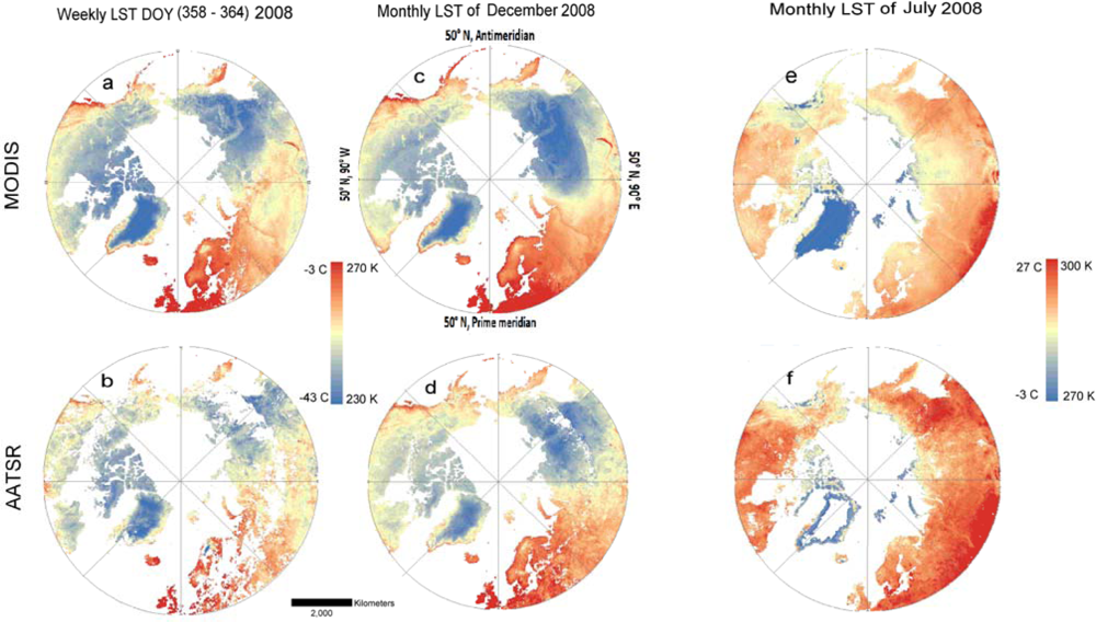
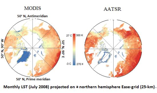
Examples of UW-L3 products are presented in Figure 2. Corresponding UW-L3 products of AATSR and MODIS were found to follow similar LST patterns. Yet, LST products of MODIS were more spatially and temporally complete than those of AATSR (Figure 2) because the number of L2 MODIS observations is approximately 10-fold that of AATSR. MODIS sensors have the advantages of being onboard of two satellite platforms, Aqua and Terra, in addition to having a larger swath than AATSR. Although at the moment the density of AATSR is low, in the future, the SLSTR (Sea and Land Surface Temperature Radiometer), which is a successor of AATSR, is to be included on the payload of the twin Sentinel-3 satellites. The satellite pair will enable a short revisit time of less than one day, which will restore the ratio between MODIS and AATSR / SLSTR observations.
The maximum count of L2 MODIS observations was found in the April to October period. Unexpectedly, this period is known to have the highest cloud cover in the high and low Arctic [52]. The minimum count occurred during the period from October to March (Figure 3), which is characterized by the existence of snow on ground. Despite the high cloud fraction during the snow-free period (June–August), clouds can be easily detected during summer because of the large difference in reflectance between land and cloud. In contrast, snow-cover interferes with the cloud masks [53,54] and causes more L2 observations to be rejected, and therefore the total number of observations to drop.
AATSR observations were found to drop significantly during the snow-free period, suggesting that AATSR cloud mask tends to reject more observations in summer (Figure 3). The total number of L2 AATSR observations increased during the year 2006 compared to the average number of L2 observation found between years 2005–2009. The most likely cause of the “false” clear-sky observations was the development of a thin coating film on the visible channel calibration. This thin film caused a drift and poor performance of the sensor and higher probability of cloud contamination during that year [55].
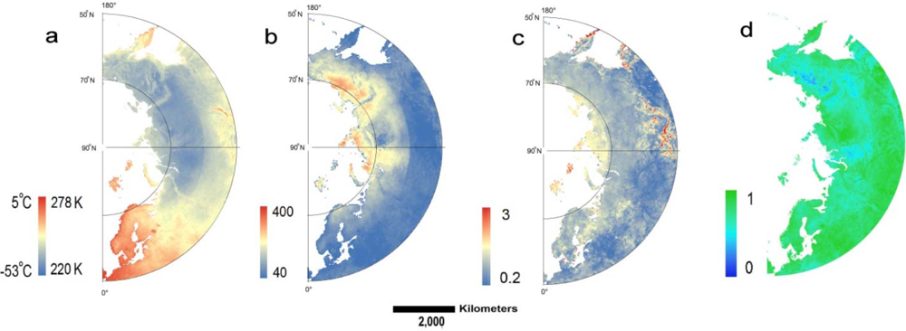
A sudden drop in LST was identified around 60°N in Eurasia and North America during the cold months, particularly evident during the months of December and January (Figure 4). The drop in LST was found to correspond to a significant loss of available L2 MODIS observations [56]. This problem has been traced back to the input L2 cloud mask (MOD35 product) resulting likely from use of latitude dependent algorithm paths to retrieve the cloud mask [57]. The issue is currently being addressed in preparation for the release of Collection 6 data expected in summer 2013 [58].

5.2. Temporal Structure of the Bias

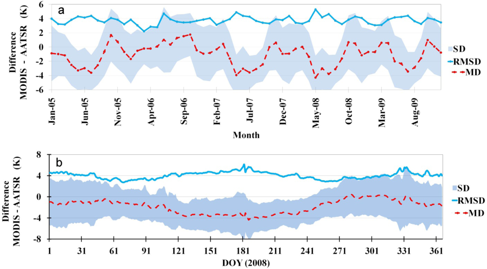
Comparison between weekly UW-L3 products of MODIS and AATSR of year 2008 indicated an annual average MD of −1.8 K (Min: −4.4 K, Max: 0.4 K) and an annual average RMSD of 4 K (Min: 2.7 K to Max: 6.1 K). Comparison of monthly products for the period 2000 to 2010 (Figure 5(a)) indicated a similar bias range of an average MD of −1.1 K (Min: −4.3 K, Max: 1.8 K) and an average RMSD of 3.8 K (Min: 2.2 K, Max: 5.3 K). Day-time averages were found to be more different (MD: −0.1 K, RMSD: 5.1 K) than night-time averages (MD: −2 K, RMSD: 3.2 K). Comparing annual products of both sensors over the 2005–2009 period showed the lowest difference with an average MD of −1.1 K (Min: −1.8 K, Max: 0.1 K) and an average RMSD of 2.1 K (Min: 1.6 K, Max: 2.8 K). The reported bias between the two sensors (AATSR and MODIS) can be attributed to differences in retrieval algorithms and density of observations (Figure 5(b)).
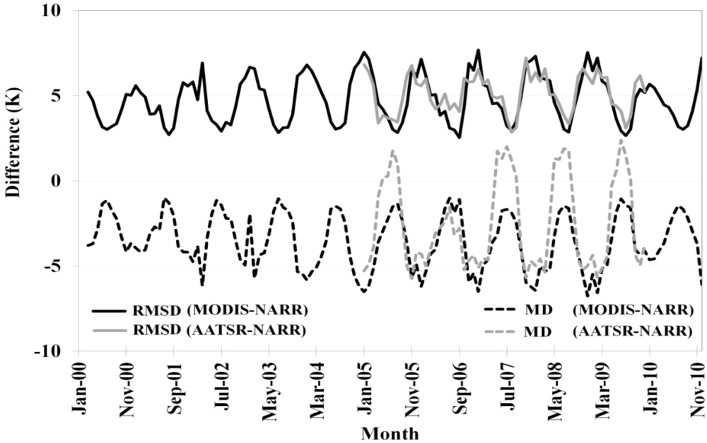
Differences between monthly UW-L3 of MODIS and NARR LST (all-sky) show an average MD of −3.6 K (Min: −6.8 K, Max: −1.0 K) and an average RMSD of 4.8 K (Min: 2.5 K, Max: 7.7 K). The results of comparing mean annual LST products estimated from MODIS and NARR over North America indicated similar bias range with a MD of −3.6 K (Min: −4.2 K, Max: −3.1 K) and a RMSD of 4.2 K (Min: 3.7 K, Max: 4.6 K). The average bias between MODIS and NARR is entirely negative. In contrast, the observed bias between monthly UW-L3 of AATSR products and NARR had positive and negative magnitudes with a MD of −2.5 K (Min: −5.8 K, Max: 2.4 K) and a RMSD of 5.1 K (Min: 2.9, Max: 7.2 K). The positive difference during summer (AATSR warmer) could be traced to overestimating LST by L2 AATSR observations [38].
The bias between monthly UW-L3 of MODIS and AATSR products and NARR (all-sky), depicted in Figure 6, is systematic during the period 2000–2010 with a maximum difference around mid-winter and a minimum around July/August of every year. However, the maximum cloud coverage during the warm period (June–August) corresponds to the minimum difference. Remarkably, the systematic bias pattern is opposite to the interannual variation of cloud cover at high latitudes (see Figure 3). The observed negative difference during the cold months (snow on ground season) suggests that the admixing of top-of-the-cloud temperatures influences the winter LST estimates more than the summer. The reported bias is not absolute. The accuracy of LST (NARR) is influenced by how accurate the land surface scheme utilized in NARR captures energy partition in higher latitudes. In addition, the number of assimilated weather stations in higher latitudes is smaller than in mid latitudes. For example, it has been reported that NARR data tend to be warmer than LST derived from SSM/I data [49].

5.3. The Bias towards Clear-Sky Observations

Different sources of bias could influence UWL3 products. We will discuss two major types of errors: the bias towards clear-sky average and the erroneous observations of undetected clouds. The bias towards clear-sky days will result in a warmer (colder) LST average during winter (summer) than the average LST for all-sky conditions (true LST mean). The cloud cover increases LST during winter by re-emitting long-wave radiation to the earth’s surface, while decreasing LST during summer by blocking direct solar radiation (increasing reflection back to space). In contrast, the bias introduced by erroneous observations of undetected clouds will always result in a negative offset of average LST because top-of-the-cloud temperatures are much colder than that of the land surface regardless of the season.
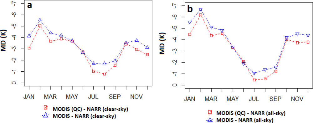
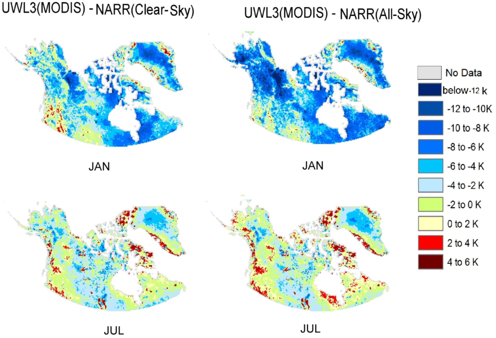
The results (Figure 7) clearly show that contamination with top-of-the-cloud temperatures (as indicated by applying a conservative quality control filter) is reduced in monthly LST averages, but it is not the main source of bias. Using a less restrictive quality control filter resulted in a negative bias between 0.5 and 1 K (relative to NARR). The bias towards clear-sky days contributed much more to the overall error, as can be seen by comparing the left and right panels of Figure 7. Adding to that, the summer bias between MODIS and NARR all-sky (Figure 7(b)) was found to be less than the summer bias between MODIS and NARR clear-sky (Figure 7(a)), likely because the positive summer bias (toward warm clear-sky days) countered the apparent negative bias during the warm months. Remarkably, the sinusoidal bias structure dominates the bias curves in both left and right figures indicating that the source of that oscillating bias is independent from errors resulting from the top-of-the-cloud admixing and from the bias towards clear-sky days. With regard to the spatial structure of error, the patterns of bias between MODIS and NARR (clear-sky vs. all-sky) during the month of July are not different; however, the difference in the severity of the bias is clear during the month of January (Figure 8).

5.4. Spatial Structure of the Bias

5.4.1. Bias between Sensors

Spatial structure of bias between UWL3 products of the two sensors (MODIS and AATSR) is different in summer compared to winter (Figure 9). The bias is more structured during the winter time. For example, regions with relatively warmer temperature and high humidity (i.e., North American west coast or Western Europe) were found to be dominated by a positive bias (MODIS warmer), while colder and dry regions were dominated by negative bias (AATSR warmer). In addition, the artifact identified in MODIS products was apparent in the winter bias map (Figure 9(a)). Bias patterns in summer (Figure 9(b)) were found to be more random, reflecting the natural heterogeneity of land cover types and lacking the contrasted patterns found during the winter. The increase in bias during summer can be attributed to: the difference in spatial resolution of land cover used to assign surface emissivity and to retrieve LST from sensor brightness temperature. The fewer AATSR observations available to calculate UW-L3 monthly means could also contributed to overestimation of LST in L2 AATSR products [38].

5.4.2. Bias between Different Datasets

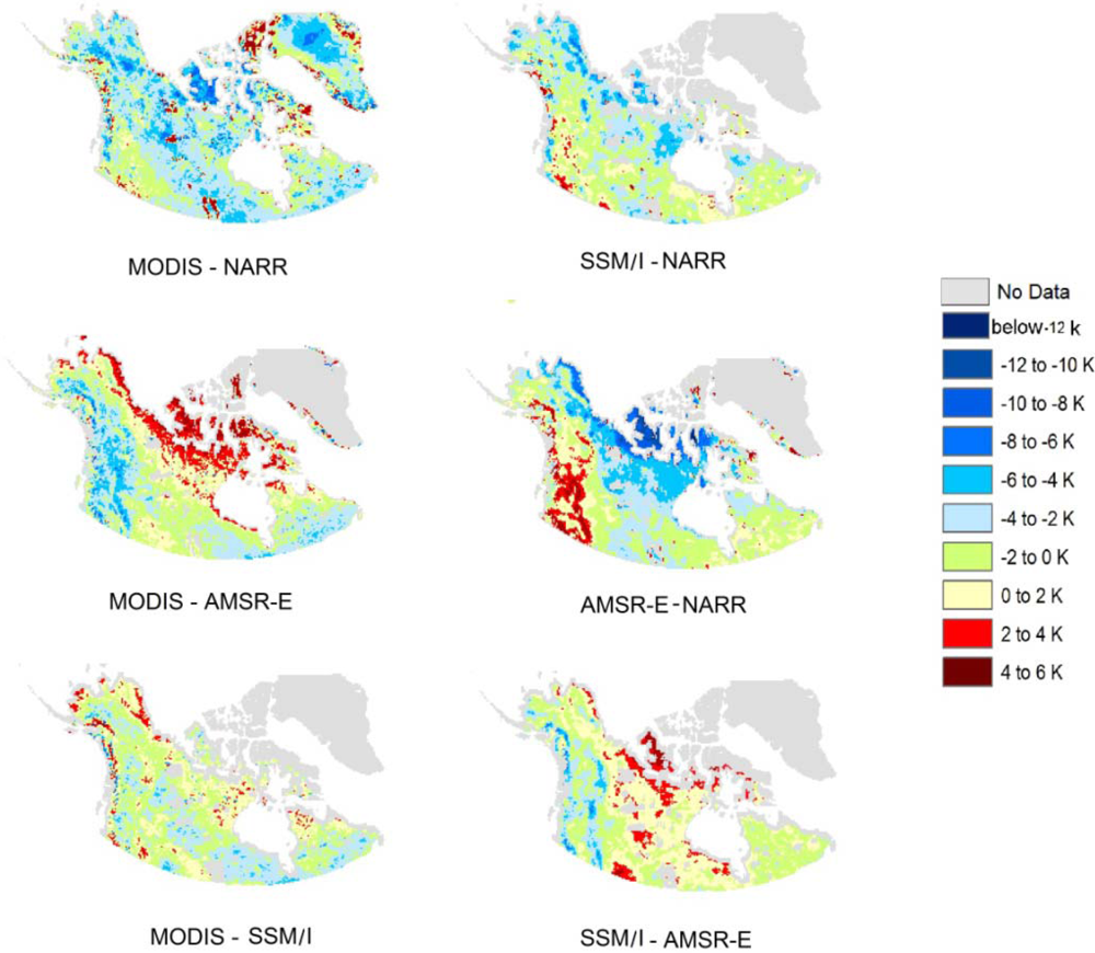
Bias patterns between monthly (clear-sky) products of different datasets during the month of July 2007 are presented in Figure 10. MODIS and SSM/I show the highest agreement of all the datasets analyzed, followed by the bias patterns between LST of SSM/I and NARR. However, the close resemblance between the SSM/I and NARR products is expected given the fact that diurnal temperature cycle of hourly NARR data was used to normalize the SSM/I measurements, see details in Royer and Poirier [49]. The bias (MD) patterns between UW-L3 of MODIS LST and NARR indicate that MODIS is colder by −2 to −4 K. Apart from that, comparing monthly near-surface air temperature of AMSR-E Ta with NARR shows a significant positive bias in mountainous regions. The high-altitude bias can be attributed to the coarse resolution of passive microwave, which does not resolve areas with complex topography. A negative bias (monthly AMSR-E Ta is colder than NARR) was observed at north latitudes. This negative bias was limited to the month of July and did not show up in the month of August (data is not presented). Melting of snow and ice, which still continues to happen at high latitudes between July and August, could interfere with passive microwave signals [59].
Spatially averaged bias (RMSD) between satellite LST products (UW-L3, SSM/I and AMSR-E) during mid-summer (July and August 2007) were found to be less than RMSD between the satellite products (SSM/I, AMSR-E and MODIS) and NARR, indicating a higher agreement between satellite products than the reanalysis (Table 4). Comparing spatially averaged bias between MODIS and clear-sky/all-sky monthly-averaged datasets during summer time indicates a background MD of −1.3 K and a RMSD of 2.9 K for comparison with clear-sky products and a MD of −1 K and a RMSD of 2.7 K for comparison with all-sky products. The background error indicates that overrepresentation of clear-sky days, did not add much bias to the summer UW-L3 estimates.
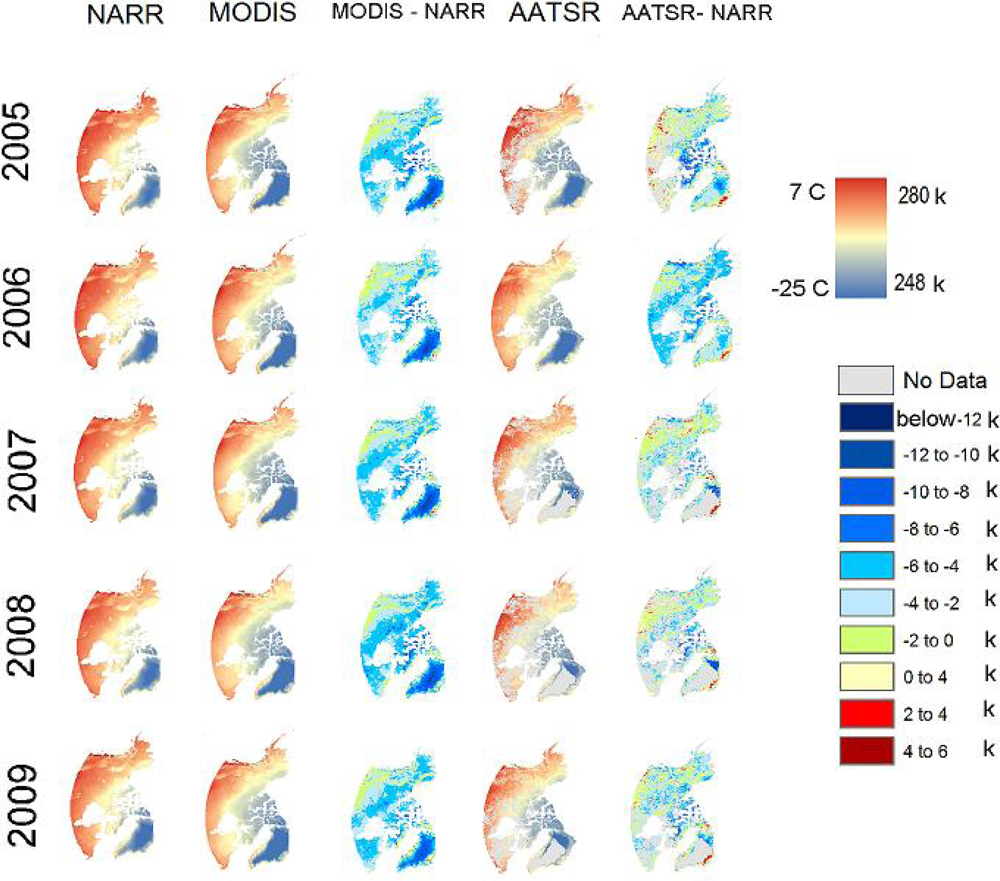
Mean annual surface temperature (MAST) is an important variable in studying different cryospheric systems such as permafrost. We derived uncertainty maps over North America showing that a RMSD of 4 K exist between UW-L3 of MODIS and NARR, while UW-L3 of AATSR differed from NARR by a RMSD of 3.5 K between, which is higher than the bias between the MAST of both sensors, 2.1 K for the period 2005–2009 (Table 5).
The distribution of bias in MAST (MODIS/AATSR-NARR) indicates an association with cold temperature, dry climate and snow-covered conditions (Figure 11). Warm regions with relatively high atmospheric humidity and temperature on average (i.e., Western North America) were found to deviate by 0 to −2 K on annual basis, with NARR being warmer. Regions which experience colder and dryer atmosphere during the Arctic winter had a negative bias reaching between −4 to −6 K (see medium blue in Figure 11). Regions, which maintain dry and cold atmosphere year around (i.e., high Canadian Arctic and central Greenland), were found to deviate the most from NARR, with bias that could reach below −6 K.
Knowing the exact atmospheric column properties (i.e., water vapor concentration and air temperature) is crucial to estimate the empirical regression coefficients (used in the split window algorithms) that relate LST to brightness temperature recorded by the TIR sensor. However, the number of Arctic radiosonde profiles available for the regression analysis in MODIS and AATSR retrieval libraries are relatively low. In addition, studies on SST retrieval have shown that split window algorithms, sometimes, perform poorly in high latitudes. During winter, ice fog and ice clouds, which are difficult to detect, interfere with IR absorption and emission [60]. Therefore, we speculate that misestimating Arctic atmosphere properties (by using atmospheric profiles from lower latitudes with relatively higher temperature and water vapor concentration) could result in the high negative bias observed during the winter. This hypothesis is consistent with the minimum bias observed during the Arctic summer because the atmosphere starts to get warmer and the water vapor reaches a higher level compared to the winter. However, a careful testing of this hypothesis is beyond the scope and focus of this paper.

6. Conclusions

Novel pan-Arctic Land Surface Temperature (LST) products were aggregated from Level 2 (L2) unprojected observations of AATSR and MODIS, separately. The new products (UW-L3) were binned on a 25 km Ease-grid at weekly, monthly and annual intervals, thereby meeting the requirements of the permafrost and the regional climate modeling communities. An intercomparison was conducted between UW-L3 products and skin temperature derived from passive microwave data (AMSR-E and SSM/I) and derived from the North American Regional Reanalysis (NARR) to assess products uncertainty. Results indicate that UW-L3 products are closely related to all datasets during the summer months with a Mean Difference (MD) of −1 K and a Root Mean Square Difference (RMSD) of 2.7 K, averaged over all geographic locations above 50 degrees north. Since other datasets represent land temperature under all weather conditions, the observed difference is partially caused by biases in original datasets and by interpolation and aggregation of UW-L3.
A systematic winter difference was found between UW-L3 of MODIS/AATSR and monthly average skin temperature derived from NARR. The bias increased gradually from summer to winter months and reached a maximum RMSD value in the middle of the Arctic winter (7.7 K for MODIS and 7.2 K and for AATSR products). One should not consider reported bias as absolute. It is recognized that NARR performance in the Arctic is influenced by the number of assimilated weather stations, which is relatively small at high latitudes. Nevertheless, the winter bias was attributed to the inclination of UW-L3 of MODIS towards clear-sky observations and admixing with top-of-the-cloud temperatures. Furthermore, we speculate that the difference between winter and summer bias range could be caused by a reduction in the efficiency of the split window algorithm (of both AATSR and MODIS) at high latitudes during Arctic winter. A careful test of this hypothesis is beyond the scope of this study. Finally, we present the following four topics, based on our reported results here that merit further investigation to improve the quality of LST products from AATSR and MODIS over the Arctic:
  • The impact of the improvement in the upcoming MODIS Collection 6 LST products in relation to the identified artifact at 60 degrees North need to be quantified and compared to current products from Collection 5.
  • The bias between UW-L3 LST products at 1-km and ground-based station measurements of both near-surface air temperature and radiometric LST measurements is unknown. Further studies are needed to quantify the magnitude and various sources of uncertainty of the 1-km products.
  • The quality of cloud masks used in L2 MODIS and AATSR LST products is a topic that merits further investigation. The influence of polar darkness and snow cover on the quality of the operational cloud mask needs to be studied and more robust algorithms need to be developed.
  • Further studies are needed to assess the performance of operational split window algorithms for both AATSR and MODIS at high latitudes during the Arctic winter.

Acknowledgments

This work was funded through ESA’s Data User Element Permafrost project (contract ESA ESRIN 22185/09/I-OL). We are indebted to Alain Royer, CARTEL, Université de Sherbrooke, Canada, for providing the SSM/I LST dataset used in this study. We also wish to thank the anonymous reviewers for their constructive comments.

References

  1. Coll, C.; Hook, S.J.; Galve, J.M. Land surface temperature from the Advanced Along-Track Scanning Radiometer: Validation over inland waters and vegetated surfaces. IEEE Trans. Geosci. Remote Sens 2009, 47, 350–360. [Google Scholar]
  2. Neteler, M. Estimating daily land surface temperatures in mountainous environments by reconstructed MODIS LST data. Remote Sens 2010, 2, 333–351. [Google Scholar]
  3. Prata, A.J. Land Surface Temperature Measurement from Space: Global Surface Temperature Simulations for the AATSR; ESA-CSIRO Atmospheric Research: Aspendale, VIC, Australia, 2002. [Google Scholar]
  4. Sobrino, J.A.; Sòria, G.; Jiménez-Muñoz, J.C.; Franch, B.; Hidalgoand, V.; Noyes, E. AATSR Derived Land Surface Temperature over a Heterogeneous Region. Proceedings of ENVISAT Symposium 2007, Montreux, Switzerland, 23–27 April 2007. ESA SP-636(CD-ROM)..
  5. Duguay, C.; Hachem, S.; Soliman, A. The DUE Permafrost Project—Land Surface Temperature Products: Overview and Cross-Comparison between MODIS and AATSR. Proceedings of the ESA Living Planet Symposium, Bergen, Norway, 28 June–2 July 2010.
  6. Jin, M.L.; Dickinson, R.E. New observational evidence for global warming from satellite. Geophys. Res. Lett 2002, 29, 1400. [Google Scholar]
  7. Comiso, J.C. Warming trends in the Arctic from clear sky satellite observations. J. Climate 2003, 16, 3498–3510. [Google Scholar]
  8. Hinzman, L.D.; Bettez, N.D.; Bolton, W.R.; Chapin, F.S.; Dyurgerov, M.B.; Fastie, C.L.; Griffith, B.; Hollister, R.D.; Hope, A.; Huntington, H.P.; et al. Evidence and implications of recent climate change in Northern Alaska and other Arctic regions. Climatic Change 2005, 72, 251–298. [Google Scholar]
  9. IPCC Core Writing Team. Contribution of Working Groups I, II and III to the Fourth Assessment Report of the Intergovernmental Panel on Climate Change. In IPCC Fourth Assessment Report: Climate Change 2007 (AR4); Pachauri, RK, Reisinger, A, Eds.; IPCC; Geneva, Switzerland, 2007. [Google Scholar]
  10. Wan, Z.; Dozier, J.A. Generalized split-window algorithm for retrieving land-surface temperature from space. IEEE Trans. Geosci. Remote Sens 1996, 34, 892–905. [Google Scholar]
  11. Hachem, S.; Allard, M.; Duguay, C. Using the MODIS land surface temperature product for mapping permafrost: an application to northern Québec and Labrador, Canada. Permafrost Periglac 2009, 20, 407–416. [Google Scholar]
  12. Hachem, S.; Duguay, C.R.; Allard, M. Comparison of MODIS-derived land surface temperatures with ground surface and air temperature measurements in continuous permafrost terrain. Cryosphere 2012, 6, 51–69. [Google Scholar] [Green Version]
  13. Marchenko, S.; Hachem, S.; Romanovsky, V.; Duguay, C. Permafrost and active layer modeling in the Northern Eurasia using MODIS Land Surface Temperature as an input data. Geophys. Res. Abstr. 2009, 11, EGU2009–EGU11077. [Google Scholar]
  14. Edwards, J.M. Simulation of land surface temperatures: comparison of two climate models and satellite retrievals. Geosci. Model Dev 2009, 2, 123–136. [Google Scholar]
  15. Jiménez, M.A.; Mira, A.; Cuxart, J.; Luque, A.; Alonso, S.; Guijarro, J.A. Verification of a clear-sky mesoscale simulation using satellite-derived surface temperatures. Mon. Weather Rev 2008, 136, 5148–5161. [Google Scholar]
  16. New, M.; Hulme, M.; Jones, P.D. Representing twentieth century space–Time climate variability. Part 1: Development of a 1961–90 mean monthly terrestrial climatology. J. Clim 1999, 12, 829–856. [Google Scholar]
  17. EarthTemp Network. Available online: http://www.earthtemp.net (accessed on 9 July 2012).
  18. Bartsch, A.; Wiesmann, A.; Strozzi, T.; Schmullius, C.; Hese, S.; Duguay, C.; Heim, B.; Seiffert, F.M. Implementation of a Satellite Data Based Permafrost Information System—The DUE PERMAFROST Project. Proceedings of the ESA Living Planet Symposium, Bergen, Norway, 28 June–2 July 2010. SP-686(CD-ROM)..
  19. Duguay, C.R.; Zhang, T.; Leverington, D.W.; Romanovsky, V.E. Remote Sensing of Permafrost and Seasonally Frozen Ground. Duguay, C.R., Pietroniro, A., Eds.; Washington, DC, USA, 2005; pp. 91–118. [Google Scholar]
  20. Heim, B.; Opel, T.; Bartsch, A. European Space Agency (ESA) Data User Element (DUE) Permafrost Documentation-Requirements Baseline Document; ESA: Vienna, Austria, 2009. [Google Scholar]
  21. Sòria, G.; Sobrino, J.A. ENVISAT/AATSR derived Land Surface Temperature over a heterogeneous region. Remote Sens. Environ 2007, 111, 409–422. [Google Scholar]
  22. Noyes, E.J.; Sòria, G.; Sobrino, J.A.; Remedios, J.J.; Llewellyn-Jones, D.T.; Corlett, G.K. AATSR land surface temperature product algorithm verification over a WATERMED site. Adv. Space Res 2007, 39, 171–178. [Google Scholar]
  23. Coll, C.; Caselles, V.; Galve, J.M.; Valor, E.; Niclòs, R.; Sánchez, J.M.; Rivas, Raul. Ground measurements for the validation of land surface temperatures derived from AATSR and MODIS data. Remote Sens. Environ 2005, 97, 288–300. [Google Scholar]
  24. Langer, M.; Westermann, S.; Boike, J. Spatial and temporal variations of summer surface temperatures of wet polygonal tundra in Siberia—Implications for MODIS LST based permafrost monitoring. Remote Sens. Environ 2010, 114, 2059–2069. [Google Scholar]
  25. Westermann, S.; Langer, M.; Boike, J. Spatial and temporal variations of summer surface temperatures of high-Arctic tundra on Svalbard—Implications for MODIS LST based permafrost monitoring. Remote Sens. Environ 2011, 115, 908–922. [Google Scholar]
  26. Westermann, S.; Langer, M.; Boike, J. Systematic bias of average winter-time land surface temperatures inferred from MODIS at a site on Svalbard, Norway. Remote Sens. Environ 2012, 118, 162–167. [Google Scholar] [Green Version]
  27. Duguay, C.; Soliman, A.; Hachem, S.; Saunders, W. Circumpolar and Regional Land Surface Temperature (LST) with Links to Geotiff Images and NetCDF Files; University of Waterloo: Waterloo, ON, Canada, 2012. [Google Scholar] [CrossRef]
  28. Wan, Z.; Zhang, Y.; Zhang, Q.; Li, Z.-L. Quality assessment and validation of the MODIS global land surface temperature. Int. J. Remote Sens 2004, 25, 261–274. [Google Scholar]
  29. Wan, Z.; Zhang, Y.; Zhang, Q.; Li, Z.-L. Validation of the land-surface temperature products retrieved from Terra Moderate Resolution Imaging Spectroradiometer data. Remote Sens. Environ 2002, 83, 163–180. [Google Scholar]
  30. Snyder, W.; Wan, Z. BRDF models to predict spectral reflectance and emissivity in the thermal infrared. IEEE Trans. Geosci. Remote Sens 1998, 36, 214–225. [Google Scholar]
  31. Wan, Z. Collection-5 MODIS Land Surface Temperature Products Users’ Guide. ICESS; University of California, Santa Barbara: Santa Barbara, CA, USA, 2007. [Google Scholar]
  32. Wan, Z. New refinements and validation of the MODIS land-surface temperature/emissivity products. Remote Sens. Environ 2008, 112, 59–74. [Google Scholar]
  33. Wan, Z.; Li, Z.-L. Radiance-based validation of the V5 MODIS land-surface temperature product. Int. J. Remote Sens 2008, 29, 5373–5395. [Google Scholar]
  34. Coll, C.; Wan, Z.; Galve, J.M. Temperature-based and radiance-based validations of the V5 MODIS land surface temperature product. J. Geophys. Res 2009, 114, D20102. [Google Scholar]
  35. European Space Agency. AATSR Product Handbook. Issue 2.2, Chapter 1. Available online: http://envisat.esa.int/handbooks/aatsr/ (accessed on 9 July 2012).
  36. Dorman, J.L.; Sellers, P.J. A global climatology of albedo, roughness length and stomatal resistance for atmospheric general circulation models as represented by the Simple Biosphere model (SiB). J. Appl. Meteorol 1989, 28, 833–855. [Google Scholar]
  37. Zeller, O.; Prata, F.; Remedios, J. Significant Improvements in the AATSR Land Surface Temperature Algorithm. Proceedings of ESA Living Planet Symposium, Bergen, Norway, 28 June–2 July 2010.
  38. Noyes, E.; Corlett, G.; Remedios, J.; Kong, X.; Llewellyn-Jones, D. An accuracy assessment of AATSR LST data using empirical and theoretical methods. Proceedings of the ENVISAT Symposium 2007, Montreux, Switzerland, 23–27 April 2007. ESA SP-636.
  39. Coll, C.; Valor, E.; Galve, J.M.; Mira, M.; Bisquert, M.; García-Santos, V.; Caselles, E.; Caselles, V. Long-term accuracy assessment of land surface temperatures derived from the Advanced Along-Track Scanning Radiometer. Remote Sens. Environ 2012, 116, 211–225. [Google Scholar]
  40. European Space Agency. MERCI Catalogue and Inventory, ENVISAT MERIS Reduced Resolution Archive. Available online: http://ats-merci-uk.eo.esa.int:8080/merci/welcome.do (accessed on 9 July 2012).
  41. Land Processes Distributed Active Archive, Data Pool; Available online: https://lpdaac.usgs.gov/lpdaac/get_data/data_pool (accessed on 9 July 2012).
  42. Luojus, K.; Pulliainen, J.; Takala, M.; Derksen, C.; Rott, H.; Nagler, T.; Solberg, R.; Wiesmann, A.; Metsamaki, S.; Malnes, E.; et al. Investigating the Feasibility of the GlobSnow Snow Water Equivalent Data for Climate Research Purposes. Proceedings of 2010 Geoscience and Remote Sensing Symposium (IGARSS), Honolulu, HI, USA, 25–30 July 2010; pp. 4851–4853.
  43. National Snow and Ice Data Center. Ease Grid Data. Available online: http://nsidc.org/data/ease/index.html (accessed on 9 July 2012).
  44. Bartsch, A. Production and Validation Report. In DUE Permafrost Project; European Space Agency: Paris, Cedex, France, 2011; Issue 1.1, Version 1. [Google Scholar]
  45. Jiménez, C.; Prigent, C.; Mueller, B.; Seneviratne, S.I.; McCabe, M.F.; Wood, E.F.; Rossow, W.B.; Balsamo, G.; Betts, A.K.; Dirmeyer, P.A.; et al. Global intercomparison of 12 land surface heat flux estimates. J. Geophys. Res 2011, 116, D02102. [Google Scholar]
  46. Mueller, B.; Seneviratne, S.; Jimenez, C.; Corti, T.; Hirschi, M.; Balsamo, G.; Ciais, P.; Dirmeyer, P.; Fisher, J.; Guo, Z.; et al. Evaluation of global observations based evapotranspiration datasets and IPCC AR4 simulations. Geophys. Res. Lett 2011, 38, L06402. [Google Scholar]
  47. Jones, L.A.; Ferguson, C.R.; Kimball, J.S.; Zhang, K.; Chan, S.K.; McDonald, K.C. Satellite microwave remote sensing of daily land surface air temperature minima and maxima from AMSR-E. IEEE-JSTARS 2010, 3, 111–123. [Google Scholar]
  48. Numerical Terradynamic Simulation Group. AMSR-E Land Parameters. Available online: http://ntsg.umt.edu/project/amsrelp#data-product (accessed on 9 July 2012).
  49. Royer, A.; Poirier, S. Surface temperature spatial and temporal variations in North America from homogenized satellite SMMR-SSM/I microwave measurements and reanalysis for 1979–2008. J. Geophys. Res 2010, 115, D08110. [Google Scholar]
  50. Mesinger, F.; DiMego, G.; Kalnay, E.; Mitchell, K.; Shafran, P.; Ebisuzaki, W.; Jović, D.; Woollen, J.; Rogers, E.; Berbery, E.H.; et al. North American regional reanalysis. Bull. Amer. Meteor. Soc 2006, 87, 343–360. [Google Scholar]
  51. Earth System Research Laboratory. NCEP North American Regional Reanalysis (NARR). Available online: http://www.esrl.noaa.gov/psd/data/gridded/data.narr.html (accessed on 9 July 2012).
  52. Eastman, R.; Warren, S. Interannual variations of arctic cloud types in relation to sea ice. J. Climate 2010, 23, 4216–4232. [Google Scholar]
  53. Istomina, L.; von Hoyningen-Huene, W.; Kokhanovsky, A.A.; Burrows, J.P. The detection of cloud free snow covered areas using AATSR measurements. Atmos. Meas. Tech 2010, 3, 1–13. [Google Scholar]
  54. Liu, Y.; Ackerman, S.A.; Maddux, B.C.; Key, J.R.; Frey, R.A. Errors in cloud detection over the Arctic using a satellite imager and implications for observing feedback mechanisms. J. Climate 2010, 23, 1894–1907. [Google Scholar]
  55. Kogler, C.; Pinnock, S.; Arino, O.; Casadio, S.; Corlett, G; Prata, F; Bras, T. Note on the quality of the (A)ATSR land surface temperature record from 1991 to 2009. Int. J. Remote Sens 2012, 33, 4178–4192. [Google Scholar]
  56. Detailed Description. Available online: http://landweb.nascom.nasa.gov/cgi-bin/QA_WWW/displayCase.cgi?esdt=MOD11&caseNum=SD_MOD11_10019&caseLocation=cases_data (accessed on 6 July 2012).
  57. Wan, Z. Personal Communication; June 2012. [Google Scholar]
  58. MODIS Land, MODIS C6 Processing Plans. Available online: http://modis-land.gsfc.nasa.gov/news.html (accessed on 6 July 2012).
  59. Pulliainen, J.T.; Grandell, J.; Hallikainen, M.T. Retrieval of surface temperature in boreal forest zone from SSM/I data. IEEE Trans. Geosci. Remote Sens 1997, 35, 1188–1200. [Google Scholar]
  60. Vincent, R.F.; Marsden, R.F.; Minnett, P.J.; Buckley, J.R. Arctic waters and marginal ice zones: 2 An investigation of Arctic atmospheric infrared absorption for advanced very high resolution radiometer sea surface temperature estimates. J. Geophys. Res 2008, 113, C08044. [Google Scholar]
Figure 1. Flow diagram of the processing chain used to produce pan-Arctic LST L3 products from original L2 un-projected LST 1-km products.
Remotesensing 04 03833f1
Figure 2. Examples of UW-L3 products: (a) and (b) weekly products of MODIS and AATSR using a sliding window (7-day average) start with DOY 358 (2008); and (cf) examples of monthly UW-L3 of MODIS and AATSR during the months of December and July 2008.
Remotesensing 04 03833f2
Figure 3. Inter-annual variability in cloud cover fraction extracted and modified from Eastman and Warren [52] (used with the permission of the American Meteorological Society) juxtaposed on average count per pixel for MODIS (a) and AATSR (b) and on bias (LST satellite-LST North American Regional Reanalysis (NARR)) for MODIS (c) and AATSR (d).
Remotesensing 04 03833f3aRemotesensing 04 03833f3b
Figure 4. Illustration of artifact found around 60 degrees N for Eurasia observed in UW-L3 products and originating from L2 MODIS LST due to problems with cloud mask (MOD35): (a) monthly LST mean of January 2006; (b) sum of day and night pixel count within January 2006; (c) the ratio of day to night observations count; and (d) cloud fraction during the month of January.
Remotesensing 04 03833f4
Figure 5. (a) Mean-difference (MD) and root-mean-square-difference (RMSD) between UW-L3 monthly LST of MODIS and AATSR data, outliers are not plotted for clarity; (b) bias (MD and RMSD) between UW-L3 weekly LST of MODIS and AATSR data during year 2008; outliers (DOY 35, 184 & 185) are excluded and replaced by interpolated values for clarity.
Remotesensing 04 03833f5
Figure 6. MD and RMSD between monthly UW-L3 of MODIS and AATSR against monthly 0-m height surface temperature of NARR (all-sky average) for the 2000–2010 period.
Remotesensing 04 03833f6
Figure 7. Monthly mean difference between quality controlled (QC) MODIS/all observations MODIS products relative to NARR during the year of 2009. Left panel (a) depicts comparison for clear-sky days, while the right side panel (b) shows the comparison for all-sky conditions.
Remotesensing 04 03833f7
Figure 8. Maps showing difference between UW-L3 of MODIS monthly LST and both clear-sky only and all-sky monthly 0-m height surface temperature from NARR (2009). Note that masking of cloudy days (i.e., clear-sky only) decreases the intensity of the bias in winter.
Remotesensing 04 03833f8
Figure 9. Maps showing difference between monthly UW-L3 (MODIS) and UW-L3 (AATSR) for the months of (a) January 2008 and (b) July 2008; The contrast between negative and positive bias patterns increases during the month of January due to differences in L2 observations density near the pole and the existence of the artifact in L2 MODIS LST at 60 degrees North. The negative bias spreads homogeneously during the month of July because of the different resolution of the emissivity maps of both products.
Remotesensing 04 03833f9
Figure 10. Bias maps derived from intercomparison between monthly UW-L3 of MODIS and clear-sky only monthly average of SSM/I, AMSR-E Ta and NARR temperature for the month of July 2007. SSM/I and MODIS were found to have the least contrasting bias zones when compared to reanalysis.
Remotesensing 04 03833f10
Figure 11. Mean annual surface temperature (MAST) calculated from monthly 0-m height surface temperature of NARR and MODIS/AATSR LST and difference between NAAR and MODIS/AATSR calculated MAST (2005–2009). For AATSR, any pixel found to have more than two missing months during one year was discarded from the calculation of MAST.
Remotesensing 04 03833f11
Table 1. Summary of accuracy assessment of L2 MODIS land surface temperature (LST) products (Collection 5) using the operational generalized split window algorithm.
MODIS ProductsLocationBias [K]Validation MethodSource
L2 TERRA & AQUACalifornia & Tibet PlateauME < 1
RMSE < 0.7
Radiative transfer model[33]
L2 TERRARice field, Valencia, SpainME = −0.29
SD = 0.06
RMSE = 0.67
Comparison with LST radiometer[34]
L2 TERRARice field, Valencia, SpainME = 0.24
SD = 0.58
RMSE = 0.63
Radiative transfer model[34]
L2 TERRA & AQUAMixed broad leaf forest, Hainich forest, GermanyME = −0.3
SD = 0.5
RMSE = 0.59
Radiative transfer model[34]
L2 TERRA & AQUAWet polygon tundra, Northern SiberiaME (weekly)
Min = −0.5
Max = +2
Comparison with thermal camera[24]
L2 TERRA & AQUAVariable moisture tundra, SvalbardME (weekly) = ±2Comparison with thermal camera[25]
L2 TERRA & AQUAVariable moisture tundra, SvalbardME = −3
Min = −6
Max = −1.5
Comparison with LST radiometer[26]
L3 TERRA & AQUAVarious land cover types, Northern Quebec and the North Slope of AlaskaCorrelation coefficient = 0.97
ME = 1.8
Comparison with 2-m height air temperature[12]
ME: mean error, SD: standard deviation, RMSE: root mean square error, Min: minimum error and Max: maximum error.
Table 2. Summary of accuracy assessment of L2 AATSR LST products using different retrieval algorithms.
LocationAlgorithmBias[K]Validation MethodSource
Homogenous rice field, Valencia, SpainOperational split window algorithmME = 3Comparison with LST radiometer[23]
Operational algorithm (vegetation fraction corrected)ME = −0.9
SD = 0.9
Comparison with LST radiometer
Emissivity dependent retrieval algorithmME = 0.3
SD = 0.9
Comparison with LST radiometer

Mixed land cover (bare soil, wheat crop)Operational algorithm daytimeME = −1
SD = 0.07
Radiative transfer model[22]
Marrakech, MoroccoOperational algorithm nighttimeME = −1.74
SD = 0.02
Radiative transfer model

Mixed land cover, Marrakech, MoroccoSplit window with nadir view1.1 ≤ RMSE ≤ 1.7Comparison with a reconstructed LST image*[21]
Split window with forward view1.6 ≤ RMSE ≤ 2.4Comparison with a reconstructed LST image
Dual angle algorithm channel 110.6 ≤ RMSE ≤ 1.3Comparison with a reconstructed LST image
Dual angle algorithm channel 120.9 ≤ RMSE ≤ 1.6Comparison with a reconstructed LST image

Homogenous rice field, Valencia, SpainOperational algorithmME = 3.5
SD = 0.6
Comparison with LST radiometer[34]
Operational algorithm (Land cover adjusted)ME = 0.16
SD = 0.51
Comparison with LST radiometer

Homogenous rice field, Valencia, SpainOperational split window algorithmOverestimated +2 to +5Long-term accuracy assessment[39]
Split window algorithm (land cover corrected)RMSE = ±0.5 to ±1.1Long-term accuracy assessment
Emissivity dependent SW algorithmRMSE = ±0.4 to ±0.6Long-term accuracy assessment
*Comparison with a reconstructed LST using a classified LANDSAT image and radiometric temperature for each class. ME: mean error, SD: standard deviation and RMSE: root mean square error.
Table 3. Summary of coarse resolution datasets.
SensorTypeProductPixel SizeTemporal ResolutionReported AccuracyAdvantagesSource
AMSRE
18.7/23.8 Ghz
H/V modes
Passive microwaveNear surface temperature (Ta)25 kmDaily during snow free period1 to 3.5 KMeasuring under clear and cloudy sky[47,48]
SSM/I 37 GHz
H/V modes
Passive microwaveLand surface temperature (LST)25 kmDaily during snow free period+0.05 °K ±1.85 °KMeasuring under clear and cloudy sky[49]
NARRAtmospheric reanalysis0 height air temperature (LST)32 kmDailyPositive bias +1 K [49]Continuous year around[50,51]
Table 4. Summary of bias statistics during the snow-free period (July and August 2007) between MODIS and other products for clear-sky and all-sky conditions.
MODIS-SSM/IMODIS-AMSR-EMODIS-NARRSSM/I-AMSR-ESSM/I-NARRAMSRE-NARR

MD [K]RMSD [±K]MD [K]RMSD [±K]MD [K]RMSD [±K]MD [K]RMSD [±K]MD [K]RMSD [±K]MD [K]RMSD [±K]
Clear-sky−0.892.56−1.062.55−2.163.38−0.192.38−1.652.98−1.653.46
All-sky−0.312.28−0.582.46−1.613.2−0.562.33−1.692.74−1.383.24
Table 5. Difference between mean annual surface temperature (MAST) estimated from monthly UW-L3 of MODIS and AATSR LST, and NARR 0-m surface temperature over North America.
Year(MODIS-NARR)(AATSR-NARR)(MODIS-AATSR)
MD [K] RMSD [K]MD [K] RMSD [K]MD [K] RMSD [K]
2005−3.844.41−2.333.56−1.82.78
2006−3.64.14−3.6140.11.63
2007−3.94.4−2.073.19−1.482.22
2008−4.164.61−2.243.41−1.462.22
2009−3.714.17−2.553.36−0.891.77