An Automated Cropland Classification Algorithm (ACCA) for Tajikistan by Combining Landsat, MODIS, and Secondary Data


Abstract
:
1. Introduction
2. Methods
2.1. Study Area
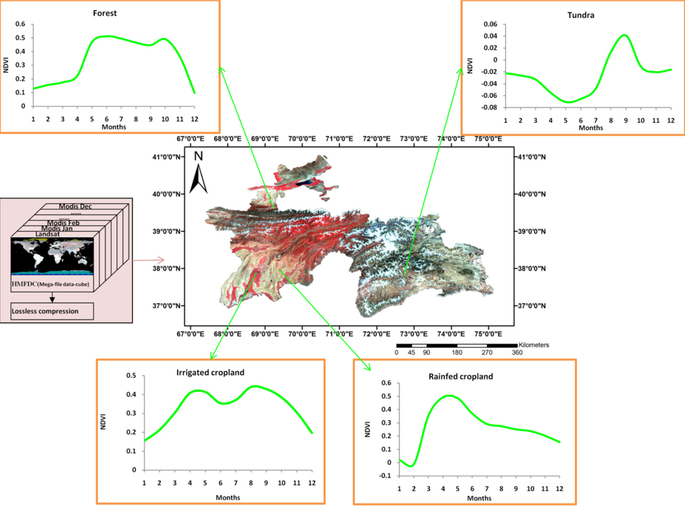
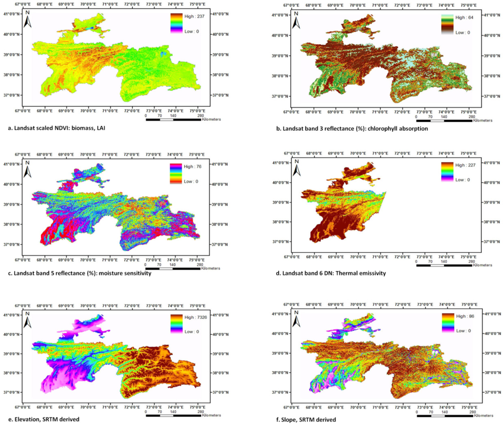
2.2. Data Fusion and Mega File Data Cubes (MFDC) Involving MODIS, Landsat, and Secondary Data
2.3. In situ Data
2.4. Algorithm Development Methods
- Generate/obtain truth/reference cropland layer (TCL): TCL can be obtained from secondary sources (e.g., from a reliable national institute such as the cropland data layer from United States Department of Agriculture). In absence of such a layer, TCL is generated using remote sensing data (see Section 2.4.1). In this study, TCLs for Tajikistan were produced for the year 2005 (TCL2005) as well as for the year 2010 (TCL2010) as described in detail in Section 2.4.1.
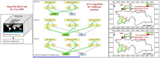
- ACCA rules and coding leading to ACCA derived cropland layer (ACL): ACCA rules are written for mega file data cube (MFDC, Section 2.2) in order to produce ACCA generated cropland layer (ACL) products that accurately replicate or come very close to replicating TCLs (within 20% quantity disagreement amongst ∼80% user’s and producer’s accuracies). The ACCA was developed for Tajikistan for the year 2005 using MFDC2005 and then applied for the year it was developed (year 2005) as well as for another independent year (year 2010). The ACCA coding process is described in detail in Section 2.4.2.
- Difference between the methods for generating TCL and ACL to demonstrate the advantage of ACL: The process of generating TCL is time consuming. For example, it involves image classification, class identification, and accuracy assessment and so on. Typical methods and approaches of generating TCLs are explained in Thenkabail and others [11]. TCLs can also be obtained from secondary sources, but they too go through time-consuming and resource-intensive processes [11]. In contrast, ACL only requires time and resource to develop the ACCA for the first year. After that the ACCA can be routinely applied for the area for which it is developed year after year to produce ACLs.
- Testing ACCA on independent data layers, comparing ACLs vs. TCLs: For Tajikistan, ACCA was developed (Section 2.4.2) using mega file data cube for year 2005 (MFDC2005). This resulted in ACCA generated cropland layer (ACL2005). ACCA is then applied to produce cropland data layers for the year for which it was developed, 2005, and for another independent year, 2010. This resulted in two ACCA generated cropland layers: ACL2005 and ACL2010. The ACLs were then tested for accuracies and errors against reference/truth cropland layers (TCLs) of corresponding years: TCL2005 and TCL2010. First for the year for which it was developed (year 2005) and then for another independent year (year 2010). This process is discussed in Section 2.4.3.
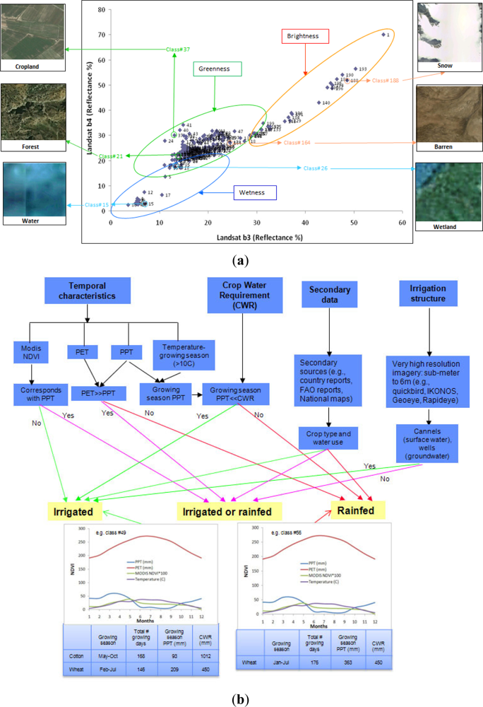
2.4.1. Producing Truth/Reference Cropland Layer (TCL)
- bispectral plots (e.g., Figure 3(a)),
- secondary data and decision trees (e.g., Figure 3(b)),
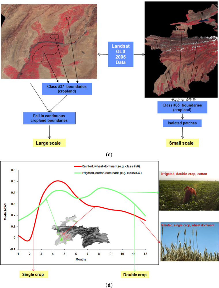
- textural characteristics (e.g., Figure 3(c)),
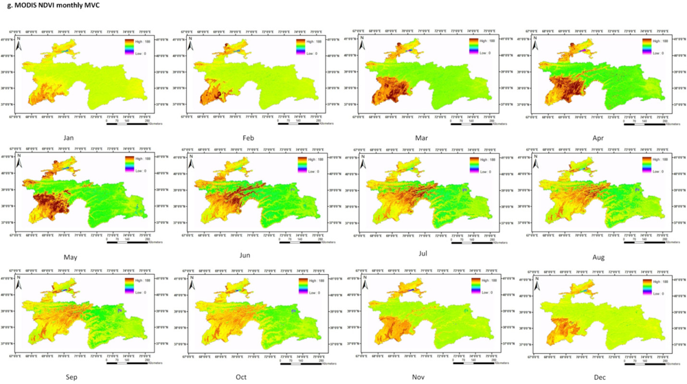
- spectro-temporal characteristics (e.g., Figure 3(d)), and
- field-plot data (e.g., Figure 3(d)) and very high resolution imagery (e.g., Figure 3(a)) involving a total of 1,770 points from precise locations (Section 2.3).
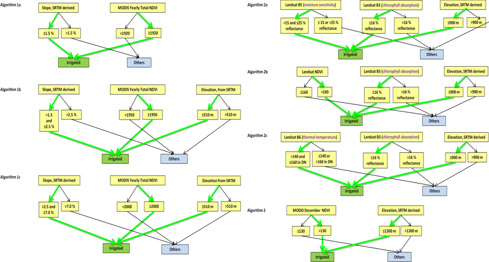
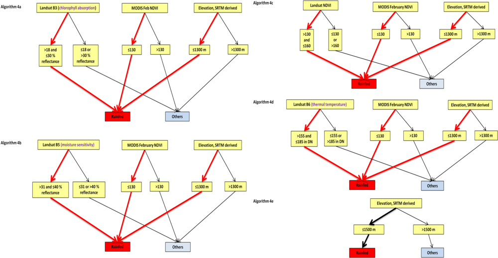
2.4.2. Automated Cropland Classification Algorithm (ACCA) Derived Cropland Layer (ACL)
2.4.3. Applying ACCA on Independent Years
3. Results and Discussions
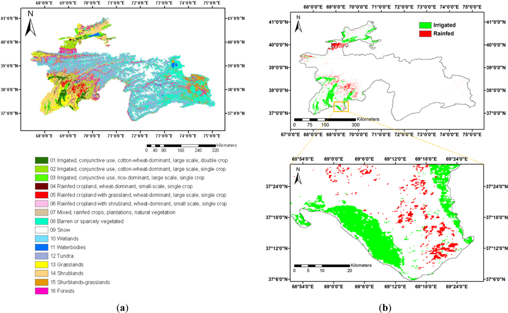
3.1. Truth/Reference Layer of Croplands for Tajikistan Based on Data for Year 2005
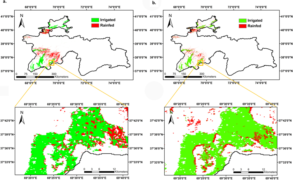
3.2. ACCA Generated Croplands (ACLs) for Tajikistan for the Same Year (2005) as That of the Truth Cropland Layer (TCL, Year 2005)
3.3. Truth/Reference Layer of Croplands for Tajikistan Based on Data for Year 2010
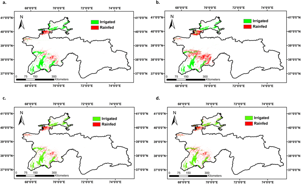
3.4. ACCA Generated Croplands for Tajikistan for the Independent Year of 2010
3.5. Accuracies and Errors
4. Uniqueness, Importance, Impact and Limitations of ACCA
4.1. The Uniqueness of ACCA Algorithm
4.2. Limitations of ACCA and the Way forward to Developing a Global ACCA
4.3. Implications and Applications of ACCA in Global Cropland Mapping
5. Conclusions and Way Forward
Acknowledgments
References
- Van den Bergh, F.; Wessles, K.J.; Miteff, S.; van Zyl, T.L.; Gazendam, A.D.; Bachoo, A.K. HiTempo: A platform for time-series analysis of remote-sensing satellite data in a high-performance computing environment. Int. J. Remote Sens 2012, 33, 4720–4740. [Google Scholar]
- Tilman, D.; Balzer, C.; Hill, J.; Befort, B.L. Global food demand and the sustainable intensification of agriculture. Proc. Natl. Acad. Sci. USA 2011, 108, 20260–20264. [Google Scholar]
- Thenkabail, P.S.; Hanjra, M.A.; Dheeravath, V.; Gumma, M. A holistic view of global croplands and their water use for ensuring global food security in the 21st century through advanced remote sensing and non-remote sensing approaches. Remote Sens 2010, 2, 211–261. [Google Scholar]
- Loveland, T.R.; Reed, B.C.; Brown, J.F.; Ohlen, D.O.; Zhu, Z.; Yang, L.; Merchant, J.W. Development of a global land cover characteristics database and IGBP DISCover from 1 km AVHRR data. Int. J. Remote Sens 2000, 21, 1303–1330. [Google Scholar]
- Friedl, M.A.; McIver, D.K.; Hodges, J.C.F.; Zhang, X.Y.; Muchoney, D.; Strahler, A.H.; Woodcock, C.E.; Gopal, S.; Schneider, A.; Cooper, A.; et al. Global land cover mapping from MODIS: Algorithms and early results. Remote Sens. Environ 2002, 83, 287–302. [Google Scholar]
- Hansen, M.C.; Defries, R.S.; Townshend, J.R.G.; Sohlberg, R.; Dimiceli, C.; Carroll, M. Towards an operational MODIS continuous field of percent tree cover algorithm: Examples using AVHRR and MODIS data. Remote Sens. Environ 2002, 83, 303–319. [Google Scholar]
- Ozdogan, M.; Woodcock, C.E. Resolution dependent errors in remote sensing of cultivated areas. Remote Sens. Environ 2006, 103, 203–217. [Google Scholar]
- Wardlow, B.D.; Kastens, J.H.; Egbert, S.L. Using USDA crop progress data for the evaluation of greenup onset date calculated from MODIS 250-meter data. Photogramm. Eng. Remote Sensing 2006, 72, 1225–1234. [Google Scholar]
- Wardlow, B.D.; Egbert, S.L.; Kastens, J.H. Analysis of time-series MODIS 250 m vegetation index data for crop classification in the US Central Great Plains. Remote Sens. Environ 2007, 108, 290–310. [Google Scholar]
- Wardlow, B.D.; Egbert, S.L. Large-area crop mapping using time-series MODIS 250 m NDVI data: An assessment for the US Central Great Plains. Remote Sens. Environ 2008, 112, 1096–1116. [Google Scholar]
- Thenkabail, P.S.; Lyon, G.J.; Turral, H.; Biradar, C.M. (Eds.) Remote Sensing of Global Croplands for Food Security; CRC Press: Boca Raton, FL, USA, 2009.
- Thenkabail, P.S.; Biradar, C.M.; Noojipady, P.; Dheeravath, V.; Li, Y.; Velpuri, M.; Gumma, M.; Gangalakunta, O.R.P.; Turral, H.; Cai, X.; et al. Global irrigated area map (GIAM), derived from remote sensing, for the end of the last millennium. Int. J. Remote Sens 2009, 30, 3679–3733. [Google Scholar]
- Xiao, X.; Boles, S.; Frolking, S.; Li, C.; Babu, J.Y.; Salas, W.; Moore, B., III. Mapping paddy rice agriculture in South and Southeast Asia using multi-temporal MODIS images. Remote Sens. Environ 2006, 100, 95–113. [Google Scholar]
- Gumma, M.K.; Nelson, A.; Thenkabail, P.S.; Singh, A.N. Mapping rice areas of South Asia using MODIS multitemporal data. J. Appl. Remote Sens 2011, 5, 053547–053547-26. [Google Scholar]
- Thenkabail, P.S.; Lyon, G.J.; Huete, A. (Eds.) Hyperspectral Remote Sensing of Vegetation; CRC Press: Boca Raton, FL, USA, 2011.
- EL-Magd, I.A.; Tanton, T.W. Improvements in land use mapping for irrigated agriculture from satellite sensor data using a multi-stage maximum likelihood classification. Int. J. Remote Sens 2003, 24, 4197–4206. [Google Scholar]
- De Fries, R.S.; Hansen, M.; Townshend, J.R.G.; Sohlberg, R. Global land cover classifications at 8 km spatial resolution: the use of training data derived from Landsat imagery in decision tree classifiers. Int. J. Remote Sens 1998, 19, 3141–3168. [Google Scholar]
- Pittman, K.; Hansen, M.C.; Becker-Reshef, I.; Potapov, P.V.; Justice, C.O. Estimating global cropland extent with multi-year MODIS data. Remote Sens 2010, 2, 1844–1863. [Google Scholar]
- Liu, J.; Shao, G.; Zhu, H.; Liu, S. A neural network approach for enhancing information extraction from multispectral image data. Can. J. Remote Sens 2005, 31, 432–438. [Google Scholar]
- Atzberger, C.; Rembold, F. Estimating Sub-Pixel to Regional Winter Crop Areas Using Neural Nets. Proceedings of ISPRS TC VII Symposium: 100 Years ISPRS–Advancing Remote Sensing Science, Vienna, Austria, 5–7 July 2010.
- Mathur, A.; Foody, G.M. Crop classification by support vector machine with intelligently selected training data for an operational application. Int. J. Remote Sens 2008, 29, 2227–2240. [Google Scholar]
- Lobell, D.B.; Asner, G.P. Cropland distributions from temporal unmixing of MODIS data. Remote Sens. Environ 2004, 93, 412–422. [Google Scholar]
- Yang, C.; Everitt, J.H.; Bradford, J.M. Airborne hyperspectral imagery and linear spectral unmixing for mapping variation in crop yield. Precis. Agric 2007, 8, 279–296. [Google Scholar]
- Chen, Z.; Li, S.; Ren, J.; Gong, P.; Zhang, M.; Wang, L.; Xiao, S.; Jiang, D. Agricultural Applications. In Advances in Land Remote Sensing: System, Modeling, Inversion and Application; Liang, S., Ed.; Springer: New York, NY, USA, 2008; pp. 397–421. [Google Scholar]
- Crist, E.P.; Cicone, R.C. Application of the tasseled cap concept to simulated thematic mapper data. Photogramm. Eng. Remote Sensing 1984, 50, 343–352. [Google Scholar]
- Cohen, W.; Goward, S. Landsat’s role in ecological applications of remote sensing. Bioscience 2004, 54, 535–545. [Google Scholar]
- Thenkabail, P.S.; Schull, M.; Turral, H. Ganges and Indus river basin land use/land cover (LULC) and irrigated area mapping using continuous streams of MODIS data. Remote Sens. Environ 2005, 95, 317–341. [Google Scholar]
- Masek, J.G.; Huang, C.; Wolfe, R.; Cohen, W.; Hall, F.; Kutler, J.; Nelson, P. North American forest disturbance mapped from a decadal Landsat record. Remote Sens. Environ 2008, 112, 2914–2926. [Google Scholar]
- Ozdogan, M.; Gutmanm, G. A new methodology to map irrigated areas using multi-temporal MODIS and ancillary data: An application example in the continental US. Remote Sens. Environ 2008, 112, 3520–3537. [Google Scholar]
- Thenkaball, P.S.; GangadharaRao, P.; Biggs, T.W.; Krishna, M.; Turral, H. Spectral matching techniques to determine historical Land-use/Land-cover (LULC) and irrigated areas using time-series 0.1-degree AVHRR pathfinder datasets. Photogramm. Eng. Remote Sensing 2007, 73, 1029–1040. [Google Scholar]
- Chan, J.C.; Paelinckx, D. Evaluation of random forest and adaboost tree-based ensemble classification and spectral band selection for ecotope mapping using airborne hyperspectral imagery. Remote Sens. Environ 2008, 112, 2999–3011. [Google Scholar]
- Goel, P.K.; Prasher, S.O.; Patel, R.M.; Landry, J.A.; Bonnell, R.B.; Viau, A.A. Classification of hyperspectral data by decision trees and artificial neural networks to identify weed stress and nitrogen status of corn. Comput. Electron. Agric 2003, 39, 67–93. [Google Scholar]
- Zheng, H.; Chen, L.; Han, X.; Zhao, X.; Ma, Y. Classification and regression tree (CART) for analysis of soybean yield variability among fields in Northeast China: The importance of phosphorus application rates under drought conditions. Agr. Ecosyst. Environ 2009, 132, 98–105. [Google Scholar]
- Thenkabail, P.S. Inter-sensor relationships between IKONOS and Landsat-7 ETM+ NDVI data in three ecoregions of Africa. Int. J. Remote Sens 2004, 25, 389–408. [Google Scholar]
- Chander, G.; Markham, B.L.; Helder, D.L. Summary of current radiometric calibration coefficients for Landsat MSS, TM, ETM+ and EO-1 ALI sensors. Remote Sens. Environ 2009, 113, 893–903. [Google Scholar]
- State Statistical Committee of the Republic of Tajikistan. Agriculture in Tajikistan. In Statistical Yearbook; Statistical Agency under President of the Republic of Tajikistan: Dushanbe, Tajikistan, 2007. [Google Scholar]
- Pontius, R.G., Jr.; Millones, M. Death to Kappa: Birth of quantity disagreement and allocation disagreement for accuracy assessment. Int. J. Remote Sens 2011, 32, 4407–4429. [Google Scholar]
- Watts, J.D.; Powell, S.L.; Lawrence, R.L.; Hilker, T. Improved classification of conservation tillage adoption using high temporal and synthetic satellite imagery. Remote Sens. Environ 2011, 115, 66–75. [Google Scholar]
- Biggs, T.W.; Thenkabail, P.S.; Gumma, M.K.; Scott, C.A.; Parthasaradhi, G.R.; Turral, H.N. Irrigated area mapping in heterogeneous landscapes with MODIS time series, ground truth and census data; Krishna Basin, India. Int. J. Remote Sens 2006, 27, 4245–4266. [Google Scholar]
- Simonneaux, V.; Duchemin, B.; Helson, D.; Er-Raki, S.; Olioso, A.; Chehbouni, A.G. The use of high-resolution image time series for crop classification and evapotranspiration estimate over an irrigated area in central Morocco. Int. J. Remote Sens 2008, 29, 95–116. [Google Scholar]
- Dheeravath, V.; Thenkabail, P.S.; Chandrakantha, G.; Noojipady, P.; Reddy, G.P.O.; Biradar, C.M.; Gumma, M.K.; Velpuri, M. Irrigated areas of India derived using MODIS 500 m time series for the years 2001–2003. ISPRS J. Photogramm 2010, 65, 42–59. [Google Scholar]
- Lv, T.; Liu, C. Study on extraction of crop information using time-series MODIS data in the Chao Phraya Basin of Thailand. Adv. Space Res 2010, 45, 775–784. [Google Scholar]
- Shao, Y.; Lunetta, R.S.; Ediriwickrema, J.; Liames, J. Mapping cropland and major crop types across the Great Lakes Basin using MODIS-NDVI Data. Photogramm. Eng. Remote Sensing 2010, 76, 73–84. [Google Scholar]
- Serra, P.; Pons, X. Monitoring farmers’ decisions on Mediterranean irrigated crops using satellite image time series. Int. J. Remote Sens 2008, 29, 2293–2316. [Google Scholar]
- Ozdogan, M. The spatial distribution of crop types from MODIS data: Temporal unmixing using Independent Component Analysis. Remote Sens. Environ 2010, 114, 1190–1204. [Google Scholar]
- Bagan, H.; Yamagata, Y. Improved Subspace classification method for multispectral remote sensing image classification. Photogramm. Eng. Remote Sensing 2010, 76, 1239–1251. [Google Scholar]
- Ramankutty, N.; Evan, A.T.; Monfreda, C.; Foley, J.A. Farming the planet: 1. Geographic distribution of global agricultural lands in the year 2000. Glob. Biogeochem. Cy 2008. [Google Scholar] [CrossRef]
- Siebert, S.; Hoogeveen, J.; Frenken, K. Irrigation in Africa; Europe and Latin America—Update of the Digital Global Map of Irrigation Areas to Version 4. Frankfurt Hydrology Paper 05; University of Frankfurt: Frankfurt am Main, Germany, 2006. [Google Scholar]
- Biradar, C.M.; Thenkabial, P.S.; Islam, M.A.; Anputhas, M.; Tharme, R.; Vithanage, J.; Alankara, R.; Gunasinghe, S. Establishing the best spectral bands and timing of imagery for land use-land cover (LULC) class separability using Landsat ETM+ and Terra MODIS data. Can. J. Remote Sens 2007, 33, 431–444. [Google Scholar]
- Wu, Z.; Thenkabail, P.S. An automated cropland classification algorithm (ACCA) by combining MODIS, Landsat, and Secondary Data for the State of California. Photogramm. Eng. Remote Sensing 2012. in review.. [Google Scholar]
- Congalton, R.; Green, K. (Eds.) Assessing the Accuracy of Remotely Sensed Data: Principles and Practices, 2nd ed.; CRC/Taylor & Francis: Boca Raton, FL, USA, 2009; p. 183.


| Satellite | Sensor | Year of Image | Spatial | Spectral | Radiometric | Band Range | Band Widths | Irradiance | Data Points | Frequency of Revisit | Usage |
|---|---|---|---|---|---|---|---|---|---|---|---|
| no unit | no unit | no unit | m | # | bit | μm | μm | W·m−2·sr−1·μm−1 | # per hectares | days | no unit |
| Landsat | ETM+ | GLS2005 | 30 | 8 | 8 | 0.45–0.52 | 0.07 | 1,970 | 11.1 | 16 | In MFDC2005 |
| 0.52–0.60 | 0.08 | 1,843 | |||||||||
| 0.63–0.69 | 0.06 | 1,555 | |||||||||
| 0.75–0.90 | 0.15 | 1,047 | |||||||||
| 1.55–1.75 | 0.2 | 227 | |||||||||
| 10.4–12.5 | 2.1 | 0 | |||||||||
| MODIS | Terra | 2005 | 250 | 36 | 12 | 0.62–0.67 | 0.05 | 1,528 | 0.16 | 1 | In MFDC2005 |
| Landsat | ETM+ | 2010 | 30 | 8 | 8 | Same as GLS2005 | Same as GLS2005 | Same as GLS2005 | 11.1 | 16 | In MFDC2010 |
| MODIS | Terra | 2010 | 250 | 36 | 12 | Same as MODIS2005 | Same as MODIS2005 | Same as MODIS2005 | 0.16 | 1 | In MFDC2010 |
| Class # | Class Name | Area | % Total Area | Landsat NDVI | MODIS NDVI Profile | |||||||||||
|---|---|---|---|---|---|---|---|---|---|---|---|---|---|---|---|---|
| 1 | 2 | 3 | 4 | 5 | 6 | 7 | 8 | 9 | 10 | 11 | 12 | |||||
| ha | no units | no units | no units | no units | no units | no units | no units | no units | no units | no units | no units | no units | no units | no units | ||
| 1 | 01 Irrigated, conjunctive use, cotton-wheat-rice-dominant, large scale, double crop | 710,166 | 5 | 0.36 | 0.09 | 0.19 | 0.28 | 0.36 | 0.37 | 0.33 | 0.36 | 0.41 | 0.39 | 0.35 | 0.28 | 0.15 |
| 2 | 02 Rainfed, wheat-barley-dominant, large scale, single crop | 273,188 | 1.9 | 0.18 | 0.05 | 0.00 | 0.31 | 0.42 | 0.47 | 0.33 | 0.26 | 0.24 | 0.22 | 0.20 | 0.18 | 0.03 |
| 3 | 03 Shrub/rangeland dominate with rainfed croplands | 470,037 | 3.3 | 0.20 | 0.01 | −0.01 | 0.22 | 0.38 | 0.39 | 0.37 | 0.29 | 0.26 | 0.23 | 0.21 | 0.09 | 0.01 |
| 4 | 04 Shrublands-grasslands | 3,384,129 | 23.6 | 0.16 | 0.02 | 0.03 | 0.12 | 0.24 | 0.24 | 0.24 | 0.21 | 0.20 | 0.18 | 0.16 | 0.07 | 0.03 |
| 5 | 05 Mixed, shrublands, grasslands, urban built-up | 70,554 | 0.5 | 0.21 | 0.01 | 0.02 | 0.20 | 0.33 | 0.34 | 0.34 | 0.29 | 0.26 | 0.24 | 0.22 | 0.16 | 0.09 |
| 6 | 06 Forest | 835,732 | 5.8 | 0.20 | 0.00 | −0.01 | 0.02 | 0.12 | 0.16 | 0.28 | 0.28 | 0.25 | 0.22 | 0.18 | 0.02 | −0.01 |
| 7 | 07 Tundra | 3,596,562 | 25.1 | 0.20 | −0.02 | −0.03 | −0.04 | −0.05 | −0.05 | 0.01 | 0.14 | 0.20 | 0.17 | 0.09 | −0.02 | −0.02 |
| 8 | 08 Wetlands | 116,386 | 0.8 | 0.21 | 0.01 | 0.02 | 0.02 | −0.05 | 0.02 | 0.15 | 0.26 | 0.25 | 0.23 | 0.20 | 0.12 | 0.00 |
| 9 | 09 Barren or sparcely vegetated | 3,380,265 | 23.6 | 0.11 | −0.01 | −0.03 | −0.02 | −0.01 | −0.02 | 0.02 | 0.08 | 0.10 | 0.09 | 0.05 | −0.01 | −0.01 |
| 10 | 10 Snow | 1,381,150 | 9.7 | 0.05 | −0.03 | −0.03 | −0.04 | −0.14 | −0.25 | −0.08 | −0.08 | −0.05 | −0.04 | −0.03 | −0.03 | −0.03 |
| 11 | 11 Waterbodies | 91,831 | 0.6 | −0.11 | −0.15 | −0.17 | −0.18 | −0.23 | −0.11 | −0.06 | −0.05 | −0.07 | −0.12 | −0.13 | −0.23 | −0.17 |
| Total | 14,218,169 | 100 | ||||||||||||||
| a. | ACCA Algorithm Derived Data for Year 2005 | ||||||
|---|---|---|---|---|---|---|---|
| TRUTH LAYER YR 2005 | Irrigated areas | Rainfed areas | All other LCLU classes | Row total | Producer’s accuracy | Errors of Omissions | |
| Irrigated areas | 7,398,009 | 152,082 | 30,326 | 7,580,417 | 97.6 | 2.4 | |
| Rainfed areas | 143,585 | 2,519,546 | 252,914 | 2,916,045 | 86.4 | 13.6 | |
| All other LCLU classes | 24,215 | 20,577 | 142,205,696 | 142,250,488 | 99.97 | 0.03 | |
| Column total | 7,565,809 | 2,692,205 | 142,488,936 | 152,123,251 | |||
| User’s accuracy | 97.8 | 93.6 | 99.8 | 152,746,950 | |||
| Errors of Commission | 2.2 | 6.4 | 0.2 | ||||
| Overall accuracy | 99.6 | ||||||
| Khat | 0.97 | ||||||
| b. | ACCA Algorithm Derived Data for Year 2010 (Landsat ETM+ 2010 and MODIS 2010) | ||||||
|---|---|---|---|---|---|---|---|
| TRUTH LAYER YR 2010 | Irrigated areas | Rainfed areas | All other LCLU classes | Row total | Producer’s accuracy | Errors of Omissions | |
| Irrigated areas | 7,258,443 | 412,788 | 325,116 | 7,996,347 | 90.8 | 9.2 | |
| Rainfed areas | 882,856 | 2719,506 | 3,917,696 | 7,520,058 | 36.2 | 63.8 | |
| All other LCLU classes | 618,103 | 1,255,142 | 178,375,106 | 180,248,351 | 99.0 | 1.0 | |
| Column total | 8,759,402 | 4,387,436 | 182,617,918 | 188,353,055 | |||
| User’s accuracy | 82.9 | 62.0 | 97.7 | 195,764,756 | |||
| Errors of Commission | 17.1 | 38.0 | 2.3 | ||||
| Overall accuracy | 96.2 | ||||||
| Khat | 0.96 | ||||||
Share and Cite
Thenkabail, P.S.; Wu, Z. An Automated Cropland Classification Algorithm (ACCA) for Tajikistan by Combining Landsat, MODIS, and Secondary Data. Remote Sens. 2012, 4, 2890-2918. https://doi.org/10.3390/rs4102890
Thenkabail PS, Wu Z. An Automated Cropland Classification Algorithm (ACCA) for Tajikistan by Combining Landsat, MODIS, and Secondary Data. Remote Sensing. 2012; 4(10):2890-2918. https://doi.org/10.3390/rs4102890
Chicago/Turabian StyleThenkabail, Prasad S., and Zhuoting Wu. 2012. "An Automated Cropland Classification Algorithm (ACCA) for Tajikistan by Combining Landsat, MODIS, and Secondary Data" Remote Sensing 4, no. 10: 2890-2918. https://doi.org/10.3390/rs4102890
APA StyleThenkabail, P. S., & Wu, Z. (2012). An Automated Cropland Classification Algorithm (ACCA) for Tajikistan by Combining Landsat, MODIS, and Secondary Data. Remote Sensing, 4(10), 2890-2918. https://doi.org/10.3390/rs4102890