Abstract
Quantitative real-time observations of a tsunami have been limited to deep-water, pressure-sensor observations of changes in the sea surface elevation and observations of sea level fluctuations at the coast, which are essentially point measurements. Constrained by these data, models have been used for predictions and warning of the arrival of a tsunami, but to date no detailed verification of flow patterns nor area measurements have been possible. Here we present unique HF-radar area observations of the tsunami signal seen in current velocities as the wave train approaches the coast. Networks of coastal HF-radars are now routinely observing surface currents in many countries and we report clear results from five HF radar sites spanning a distance of 8,200 km on two continents following the magnitude 9.0 earthquake off Sendai, Japan, on 11 March 2011. We confirm the tsunami signal with three different methodologies and compare the currents observed with coastal sea level fluctuations at tide gauges. The distance offshore at which the tsunami can be detected, and hence the warning time provided, depends on the bathymetry: the wider the shallow continental shelf, the greater this time. Data from these and other radars around the Pacific rim can be used to further develop radar as an important tool to aid in tsunami observation and warning as well as post-processing comparisons between observation and model predictions.
1. Introduction
The highly infrequent and transient nature of tsunamis and their lack of predictability make their approach to the shore difficult to study in detail. Generally, only point measurements of wave height and water column pressure are available. Barrick [1] elucidated the mechanism whereby coastal HF radars could observe a tsunami via its current flow pattern. Subsequent analysis refined this concept and a pattern-recognition algorithm was proposed [2] that could be employed using a single radar to detect a tsunami among the background currents. The HF radar technique has the advantage of providing details of the transient current flows over wide areas of the coastal ocean with varying water depths. Because a tsunami is a rare event, prior work was based on theory and simulations. As the number of HF radar worldwide grew and real time networks were developed, the probability of detection has risen significantly. Here we report observations made by five radars located in Japan and California during the 11 March 2011 tsunami in the Pacific. We show that the HF radar systems have indeed detected and measured tsunami current flows, representing the first such tsunami observation with any radar. Further study is ongoing using data from the many coastal radars on the shores of the North Pacific.
We examine data from radars [3] on the coastlines of Japan and California at sites indicated in Figure 1(a). The data sets were obtained at 4-minute intervals using three different radar transmit frequencies: 5 MHz, 13.5 MHz and 42 MHz. Three methods were employed in the data processing, the first based on direct observation of current velocities measured by a radar pair, the second based on analysis of the radial current components from a single radar, the third based on frequency shifts in the Doppler spectrum of the radar sea echo; the methods and results obtained are described below. As expected, the measured current velocities oscillate with the period of the tsunami as derived from the surface height measurements. The tsunami was detected by the radars between 10 and 45 minutes prior to its arrival at neighboring tide gauges; possible reasons for the offset are proposed. We find that signals are detectable once the tsunami reaches the continental shelf, even after crossing the Pacific, a travel time of 9 hours. The oscillations are most coherent near the epicenter and we obtain clear and detailed current velocity maps from Hokkaido, at a range of 425 km from the epicenter of earthquake and out of the direct line of sight to it (Figure 1(b)). This is the closest known operating HF radar to the epicenter.
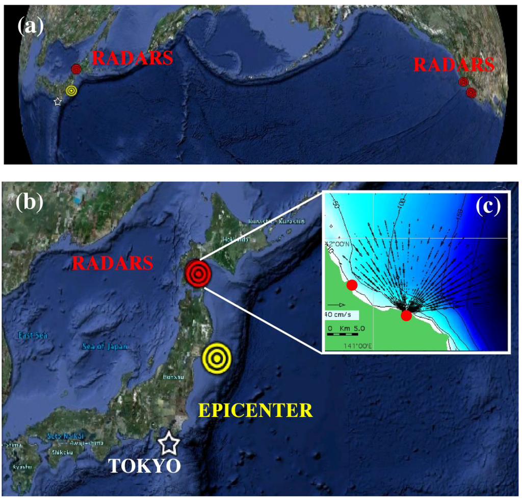
Figure 1.
(a) The North Pacific Ocean showing the location of the radars in Japan and California that provided data for this paper; (b) The location of the Japan earthquake and the radars in Hokkaido; (c) The bathymetry offshore from the radars and radial velocities measured by the Kinaoshi radar, 11 March 2011, 21:00 JST.

In addition to their primary operational purpose of observing real-time offshore circulation [4,5], the radars can also provide local quantitative tsunami information and warning as the actual wave approaches. There are over 80 HF radars operating on the US Pacific coast located 8,000–8,500 km from Japan; most are suitable for observing the tsunami signature, although they may not have been configured to record the appropriate data. This provides the opportunity to study variations of the tsunami signature by analyzing data from a number of sites. A more detailed analysis of their weaker signals will allow a unique view of the propagation of the tsunami and its interaction with the ocean floor for comparison with computer models. Here we report the general features of the data from three sites.
Because of the diversity in local bathymetry, there is considerable variation in the warning time available, primarily depending on the width of the adjoining continental shelf, varying from minutes on the US Pacific coast to hours for some areas of the Atlantic coast and South East Asia. As we relate the detection time to the water depth at the observation point, observations of the Japan tsunami allow us to obtain accurate estimates of the warning time for other bathymetry. The characteristics of the current fields can also be used to develop improved detection algorithms.
2. Tsunami Theory
A tsunami anywhere on the ocean is a shallow-water gravity wave; i.e., its wavelength is much greater than the water depth. It is the linear solution of the Laplace equation with kinematic boundary conditions at the surface, giving two equations of motion. Kinsman ([6] Section 3.5) shows that the height in water of depth is related to the height over the deep ocean basin (e.g., at ~4,000 m depth) through an inverse fourth-power relation:
This assumes the bottom is flat or is gently sloping when viewed over distances having scales equal to its wavelength λ or greater. The tsunami is forced by the refractive properties of the depth to propagate perpendicular to the large-scale bathymetry contours, traveling toward the shallower regions. The phase velocity of this wave in shallow water is independent of the wave period P, and its dispersion relation is given in terms of the acceleration of gravity g by:
Typical phase velocities for tsunamis on the open ocean are hundreds of kilometers per hour.
The velocity observed by an HF radar is not its phase speed given above, but the water particle (orbital) velocity vo. The latter is the velocity at which the Bragg-scattering waves are transported. For any ocean wave, deep or shallow, this is related to its height through the equations of motion. For deep water, the orbits are circles with radii equal to the wave height. For shallow water, they become flattened ellipses that collapse into horizontal back/forth trajectories in the very-shallow limit. This is the case for tsunamis. The horizontal orbital velocity then becomes:
This can also be expressed in terms of the deep-water height to illustrate how it changes with depth:
Equation (3) relates the tsunami height to its orbital velocity along the propagation direction and applies to a traveling wave. A coastal boundary condition modifies this traveling wave depiction as shore is approached, where Equation (3) is not expected to apply. The actual boundary condition depends on local details of the coast, but lies between two extremes [7]: (a) Perfect reflection, as from a vertical cliff. Here the normal velocity must be zero as a standing wave is created between the incident and reflected rays, while the height of this standing wave at the boundary is double that of the incoming traveling wave at that approximate depth; (b) A radiation condition, meaning the shoreward traveling wave produces no reflection. A gently sloping beach profile has this classic behavior. The height shows no appreciable change over its value for the solitary traveling wave, except for its inverse one-quarter law depth dependence. The boundary condition that actually applies at the coast is somewhere between (a) and (b).
We highlight two important points from the above equations: First from Equation (4), the velocity observed by the radar increases much more rapidly as depth decreases than the height: the latter has an inverse 1/4 power relation to depth while the velocity increases as the inverse 3/4 power. Although neither height nor orbital velocity may be appreciable in the deep ocean basin, as the tsunami moves onto the continental shelf the velocity increase that the radar observes grows more rapidly while the height increase is slower. Second from Equation (3), if the radar observes velocity at a point offshore in water depth , then the tsunami height can immediately be determined at that point. Furthermore, closer to the shore, the slowly increasing height can be roughly predicted via Equation (1) up to the point that the coastal boundary condition applies, as discussed on the preceding paragraph. This assumes linear wave theory will apply, and this holds up to depths of a couple meters [2], beyond which nonlinear runup and breaking determine final coastal impact. Thus the offshore radar-observed tsunami velocity can yield useful warning information on the expected impacts, for rapid dissemination to nearby coastal areas.
3. Detection of the Tsunami Signal in HF Radar Data
The surface current velocities seen by HF radars are derived from radar echo from ocean waves with wavelengths that are half the radar wavelength (i.e., Bragg scatter). Typically these waves have periods between 1.5 and 4.5 seconds. On the other hand, a tsunami is characterized as a shallow-water ocean wave with a period between 25 and 50 minutes. It is usually visualized [1] as a series of crests and troughs with open-ocean wavelengths of 400–800 km corresponding to their long temporal periods. These waves are accompanied by “orbital” velocities, as described above. These tsunami orbital velocities appear as large area back-and-forth flows at the surface and impart additional velocities to the short Bragg waves that are seen by the radar. In deep water, these tsunami-induced velocities fall below a detectable threshold for HF radars, but as the depth of the continental shelf decreases to about 200 m or less, they increase and can be observed by coastal HF radars.
3.1. Analysis of Measured Current Velocities
Here we examine the current velocity patterns as measured by the radars. Each radar maps the components of the current velocity radial to the radar site over the field of view [8]. With two or more nearby radar sites, these components can be combined to give an estimate of the total velocity vector [8].
3.1.1. Observations of Total Velocity Current Maps
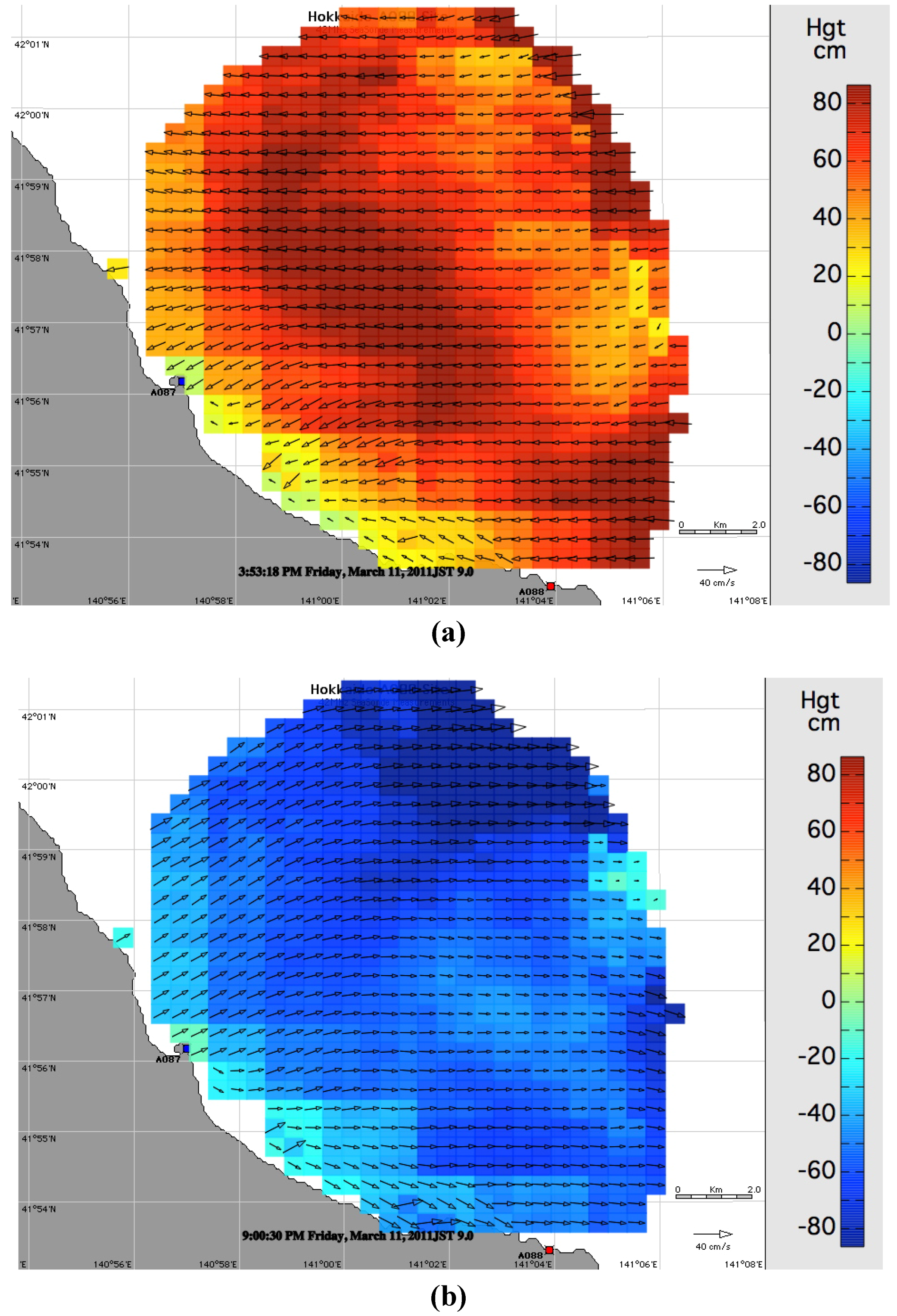
As our first example, we analyzed data from two radars located near Usujiri and Kinaoshi, Hokkaido, Japan, Figure 1(b,c). The radars have a transmit frequency of 42 MHz and a range increment of 0.5 km with a total range of 15 km. The water depth over the total radar coverage area is less than 200 m. Figure 1(c) shows an example of radial current velocities measured at Kinaoshi. The current flow from 11 March, 14:06 JST to 12 March, 13:54 JST is shown in a video clip (see supplementary media file); the earthquake occurred on 11 March 14:46 JST. The direction and strength of the flow was measured at approximate 4-minute intervals with a cell resolution of 0.5 km × 0.5 km. The maps, which display the tsunami current superimposed on the normal background flow, show the tsunami sweeping in and out of Uchiura Bay. Equation (3) relates the tsunami height and current velocity. In general, to obtain the tsunami height from Equation (3), the long-term trends need to be subtracted from the velocities to reduce the effects of the normal background flow. We chose two times for which the tsunami current appears to dominate the background flow, the first signals the tsunami arrival with inward flow, the second with strong outward flow. Figure 2 shows the tsunami height superimposed on the total current velocity field at these two times. As noted in Section 2, the height estimates from Equation (3) are not expected to be accurate very close to the shore.

Figure 2.
The tsunami height superimposed on the total current velocity field measured by radars at Usujiri (blue dot) and Kinaoshi (red dot): (a) 11 March 2011, 15:53 JST; (b) 11 March 2011, 21:00 JST.
Figure 2.
The tsunami height superimposed on the total current velocity field measured by radars at Usujiri (blue dot) and Kinaoshi (red dot): (a) 11 March 2011, 15:53 JST; (b) 11 March 2011, 21:00 JST.
3.1.2. Observations of Radial Velocity Components
The tsunami signal is also visible in the radar return from a single radar site. We use a simplified model to demonstrate the basic behavior. Assuming that the water depth over the radar coverage area can be adequately represented by parallel depth contours, a tsunami will move perpendicular to these contours. To detect the approach, the radial velocity component was resolved perpendicular to the depth contours, as described by Lipa et al. [2], averaged over bands parallel to the depth contours and plotted vs. time from the earthquake for Japan sites, or from a time just prior to arrival for US sites. These velocities were compared with tide gauge measurements of water level.
This method was applied to data from the radar at Kinaoshi, Figure 3 shows the location of the radar and tide gauge and the offshore bathymetry. Figure 4(a,b) shows the averaged radial velocity component for Kinaoshi, for six 2-km bands ranging from 2 km to 14 km from the shore. Tidal effects are also evident in the resulting velocity components: the arrival of the tsunami causes marked oscillations, which are superimposed on the normal tidal background. Figure 4(c) shows the water levels measured by a tide gauge at Hakodate, about 35 km southwest of the radar site; these data were provided by the Japan Meteorological Agency. The details of the radar and tide gauge plots differ, which is to be expected as height and current are not in phase with each other, but are determined by boundary conditions at the coast. In particular, the velocity oscillations begin about 43 minutes before the measured water level oscillations. Reasons for this effect are discussed in Section 3.3.
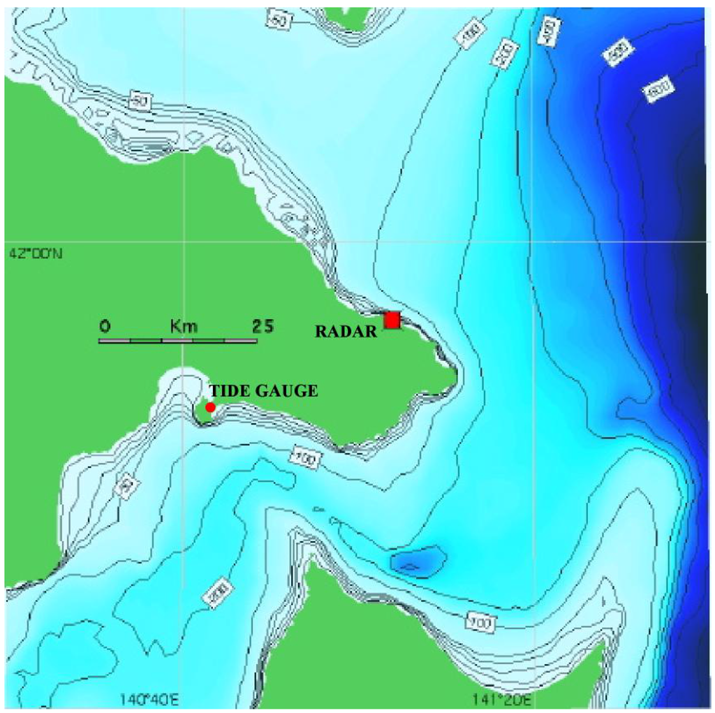
Figure 3.
The bathymetry offshore from the radar at Kinaoshi and the tide gauge at Hakodate.
Figure 3.
The bathymetry offshore from the radar at Kinaoshi and the tide gauge at Hakodate.

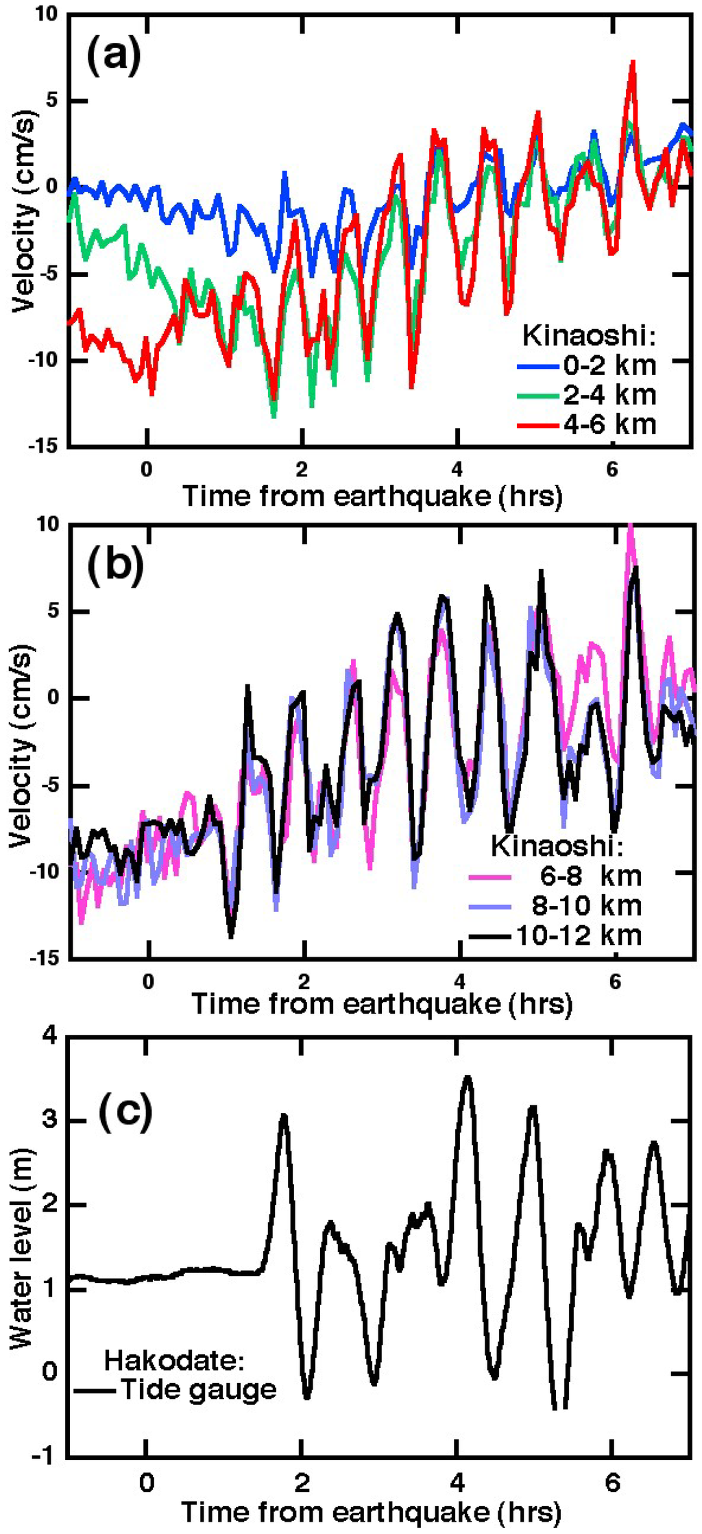
Figure 4.
Time series of velocity components from the Kinaoshi radar (42 MHz transmitter frequency) and simultaneous water level observations from the Hakodate tide gauge. Radial velocity was resolved perpendicular to the shore, and averaged over bands 2 km wide parallel to the depth contours.
Figure 4.
Time series of velocity components from the Kinaoshi radar (42 MHz transmitter frequency) and simultaneous water level observations from the Hakodate tide gauge. Radial velocity was resolved perpendicular to the shore, and averaged over bands 2 km wide parallel to the depth contours.
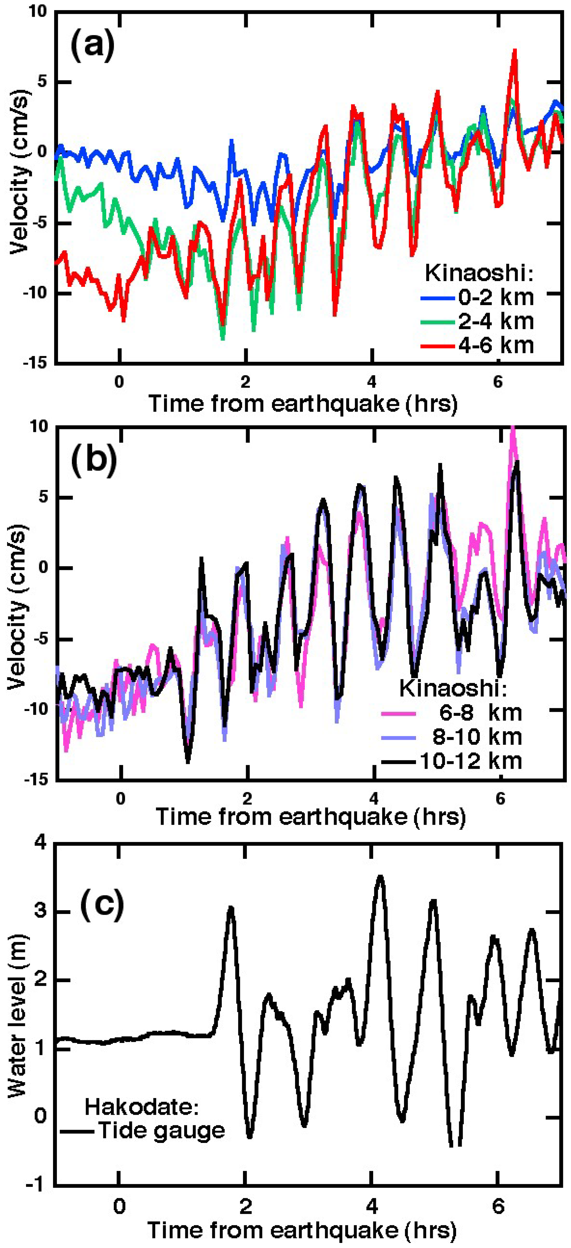
Tidal current velocities normal to the depth contours are most evident before the arrival of the tsunami, and as expected increase roughly linearly with range with the weakest current velocities close to the shore, decreasing to zero at the shoreline. The arrival of the tsunami is indicated by the commencement of distinctive oscillations in velocity, which appear to be approximately coherent with a period of about 40 minutes.
We also examined the effect of the tsunami on radial velocities measured on the western US coast and compared the results with tide-gauge measurements of water level obtained by NOAA’s Center for Operational Oceanographic Products and Services (http://tidesandcurrents.noaa.gov/).
Figure 5 shows the location of the radar at Bodega Bay, California and the offshore bathymetry. A measured radial velocity map is shown, with a reverse flow generated by the tsunami in the inner range cells. The radar has 13 MHz transmit frequency and 2 km range increments.
Figure 6(a,b) shows the component of the radial velocity perpendicular to the shore averaged over four 2-km bands ranging from 0 to 8 km from shore. Figure 6(c) shows the water levels measured by a tide gauge at Pt. Reyes, about 40 km south of the radar site. The radar detects the tsunami about 12 minutes before the tide gauge, at approximately 16:00 UTC.
As a third example, we analyzed the data from the radar at Trinidad River, California. Figure 7 shows the location, offshore bathymetry and a measured radial velocity map. We again see the reverse flow generated by the tsunami in the inner range cells. This is a long-range radar with 5 MHz transmit frequency and 6-km range increments. Figure 8(a,b) shows component of the radial velocity perpendicular to the shore for four 4-km bands ranging from 0 to 16 km from shore. Figure 8(c) shows the water levels measured by a tide gauge at Crescent City, about 70 km north of the radar site. The radar detects the tsunami about 14 minutes before the tide gauge, at approximately 16:00 UTC, as at Bodega Bay.

Figure 5.
The location of the radar at the Bodega Marine Lab., California, the offshore bathymetry and a measured radial velocity map. Measured radial velocities are for 11 March 2011, 16:52 UTC, and show the reverse flow generated by the tsunami in the inner range calls.
Figure 5.
The location of the radar at the Bodega Marine Lab., California, the offshore bathymetry and a measured radial velocity map. Measured radial velocities are for 11 March 2011, 16:52 UTC, and show the reverse flow generated by the tsunami in the inner range calls.
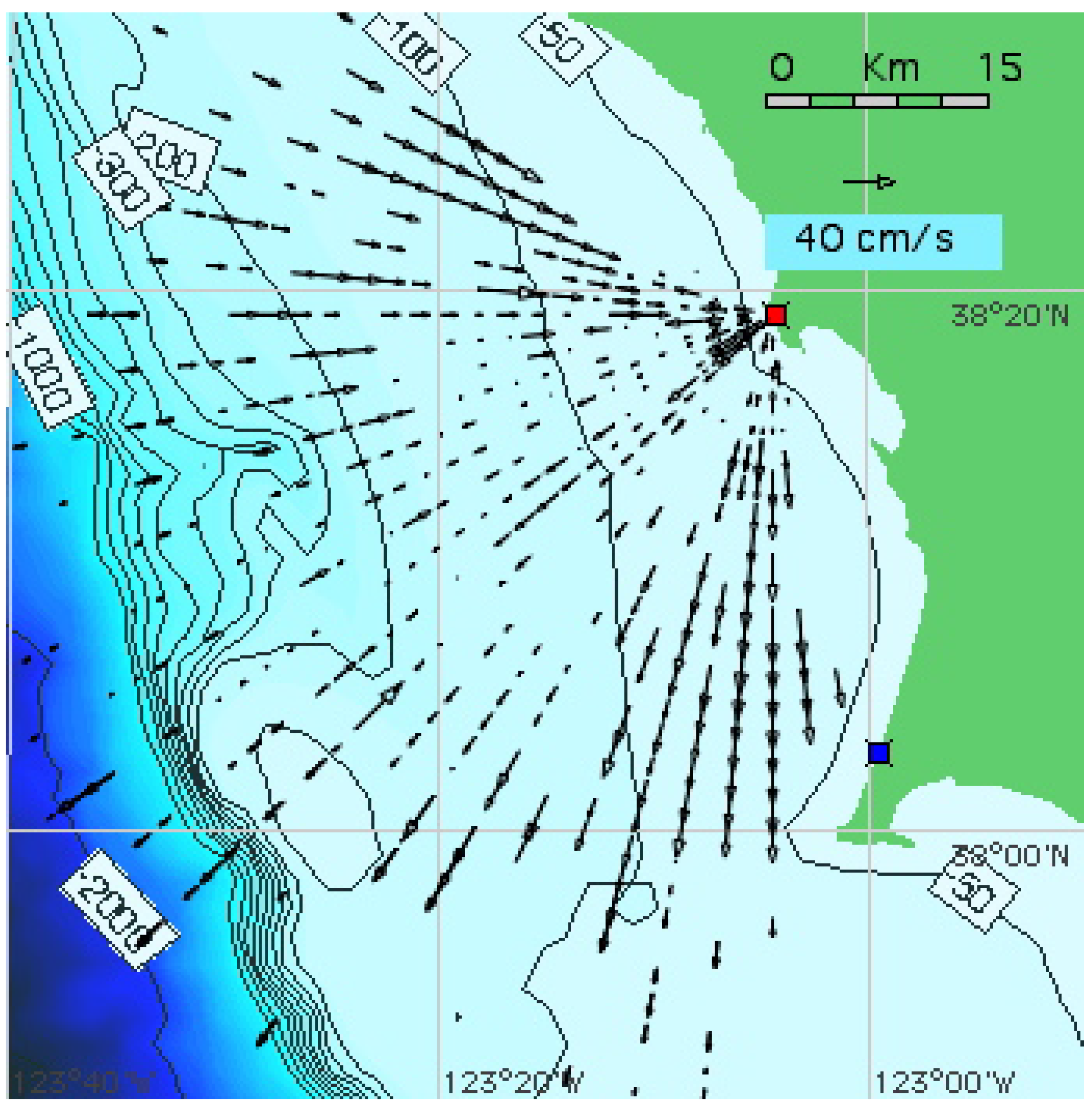
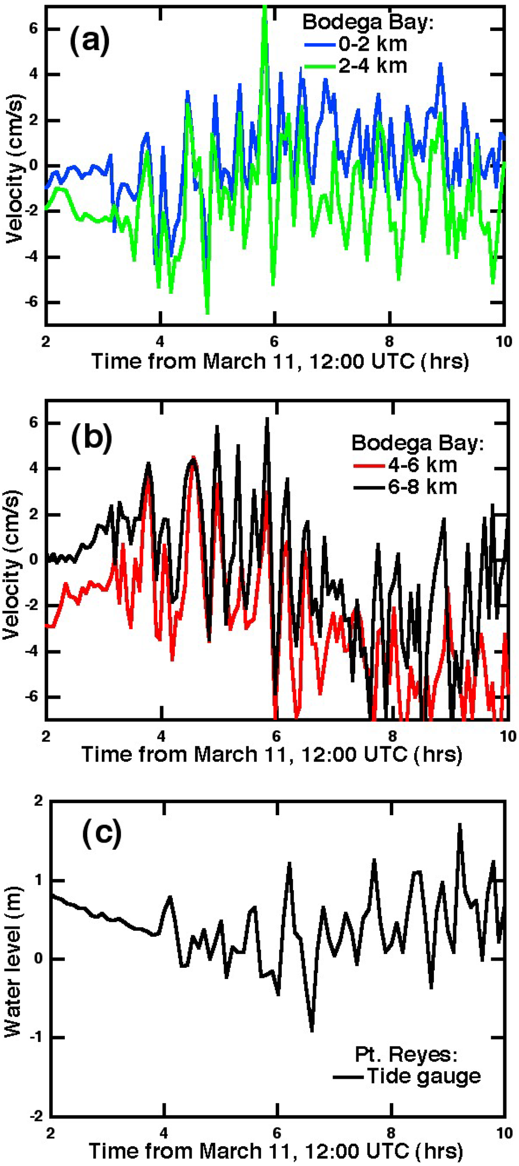
Figure 6.
Time series of velocity components from the radar at Bodega Bay and simultaneous water level observations from the Point Reyes tide gauge. Radial velocities were resolved perpendicular to the shore, and averaged over bands 2-km wide parallel to the shore.
Figure 6.
Time series of velocity components from the radar at Bodega Bay and simultaneous water level observations from the Point Reyes tide gauge. Radial velocities were resolved perpendicular to the shore, and averaged over bands 2-km wide parallel to the shore.

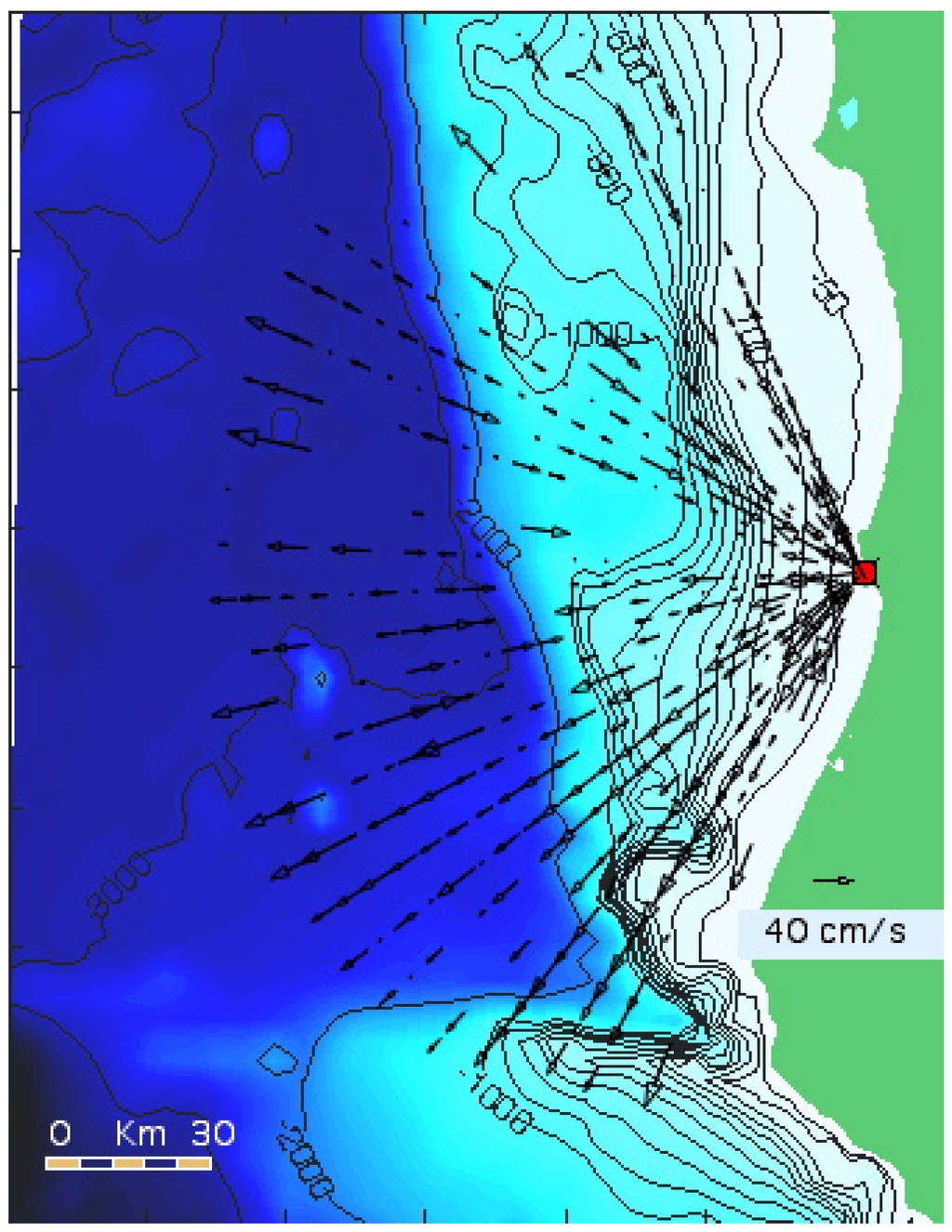
Figure 7.
The location of the radar at Trinidad River, California, the offshore bathymetry and a measured radial velocity map. Measured radial velocities are for 11 March 2011, 17:36 UTC, and show the reverse flow generated by the tsunami in the inner range calls.
Figure 7.
The location of the radar at Trinidad River, California, the offshore bathymetry and a measured radial velocity map. Measured radial velocities are for 11 March 2011, 17:36 UTC, and show the reverse flow generated by the tsunami in the inner range calls.

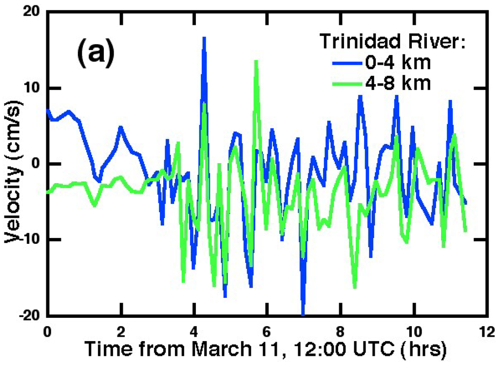
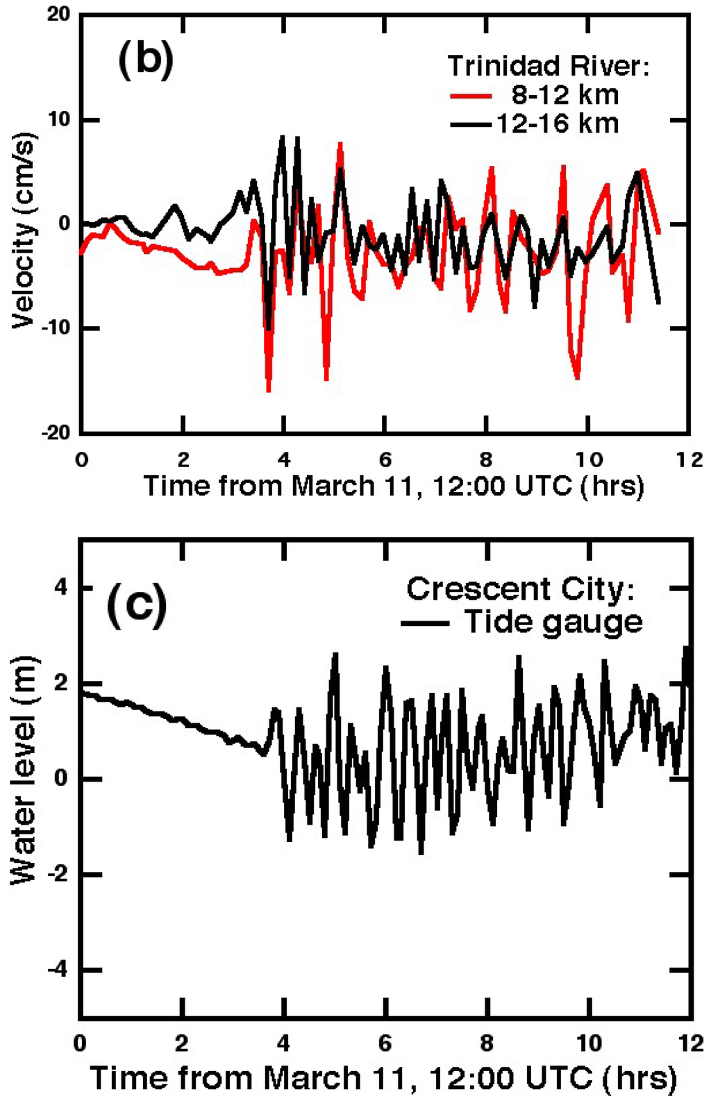
Figure 8.
Time-series of radial velocities measured by the long-range radar at Trinidad River and simultaneous water level observations from the Crescent City tide gauge. Radial velocities were resolved perpendicular to the shore, and averaged over bands 4-km wide parallel to the shore.
Figure 8.
Time-series of radial velocities measured by the long-range radar at Trinidad River and simultaneous water level observations from the Crescent City tide gauge. Radial velocities were resolved perpendicular to the shore, and averaged over bands 4-km wide parallel to the shore.


3.2. Analysis of the Radar Frequency Spectrum
It is also possible to extract tsunami information directly from the Doppler frequency spectrum of the radar echo before the compilation of current velocity maps. We examined the shift in the centroid frequency of the Bragg-echo spectral peak from the ideal Bragg frequency to give an estimate of the radial velocity over a radar range cell, which is a circular annulus of constant range and width. Figure 9 shows the location of the radar near Bolinas, California and the offshore bathymetry. The radar has 13 MHz transmit frequency and 3-km range increments.
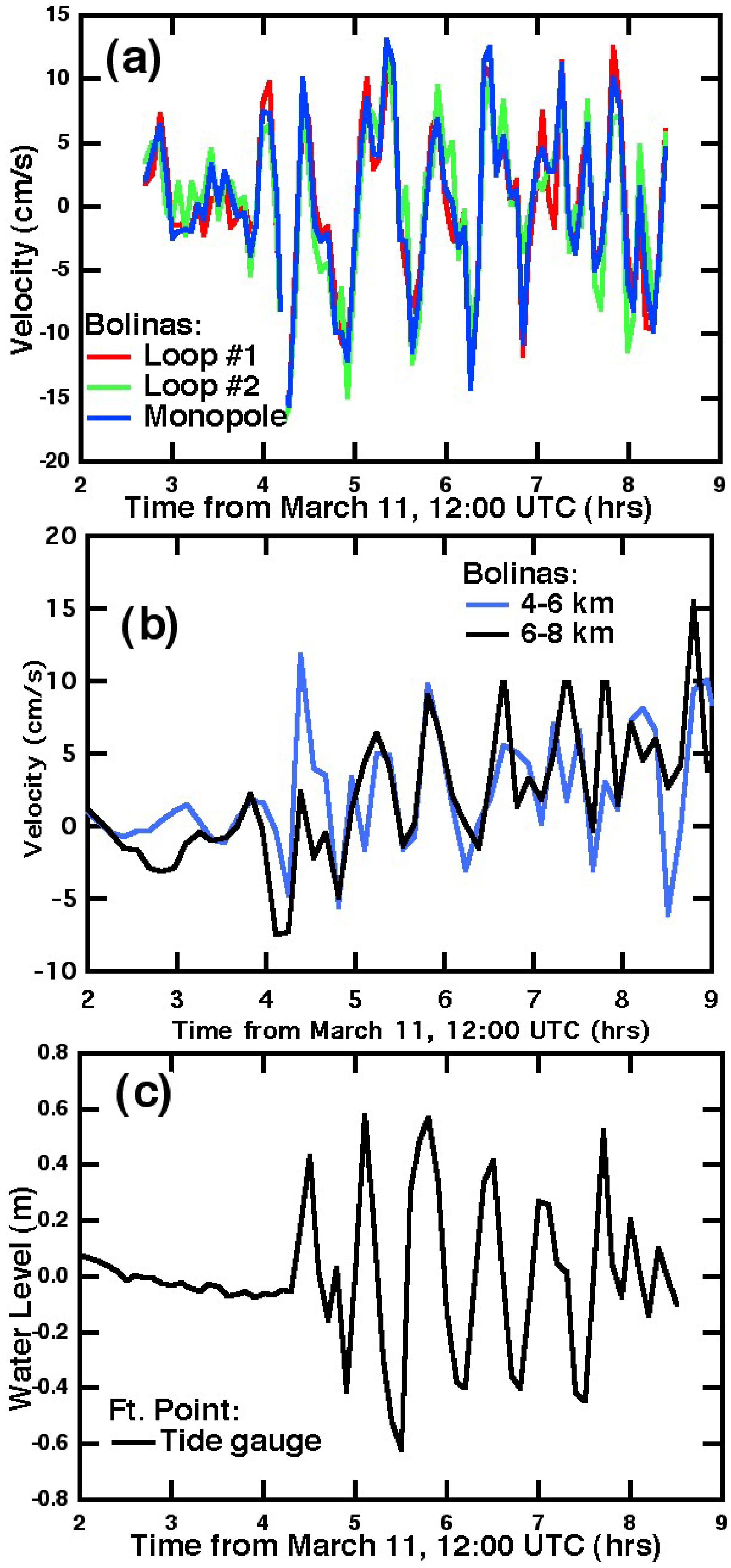
Figure 10(a) shows a plot of estimated centroid velocity for the three radar antenna signals [8] (two co-located crossed loops and a monopole) from 14:00 to 20:30 UTC, 11 March. Radar echoes came from a range cell 3 km wide and 9 km offshore with water depths ranging from 20 to 50 m. The figure shows the onset of the velocity variations due to the tsunami beginning about 16:00 UTC with oscillations up to 25 cm/s. Figure 10(b) shows the component of the radial velocity perpendicular to the shore averaged over two 2-km bands ranging from 4 to 8 km from shore, showing similar oscillations as Figure 10(a) and indicating the same arrival time. Details differ between Figure 10(a) and 10(b) due to differences between the analysis methods used and the area covered. Figure 10(c) shows the water height measured by the tide-gauge at Fort Point, California, 25 km from the radar; both show variations with periods between 15 and 45 minutes. The radar detects the tsunami about 30 minutes before the tide gauge; reasons for this are discussed in the next section. In Figure 10(a,c), tidal effects and other longer-term trends have been removed, to make the tsunami-induced current velocities more evident.
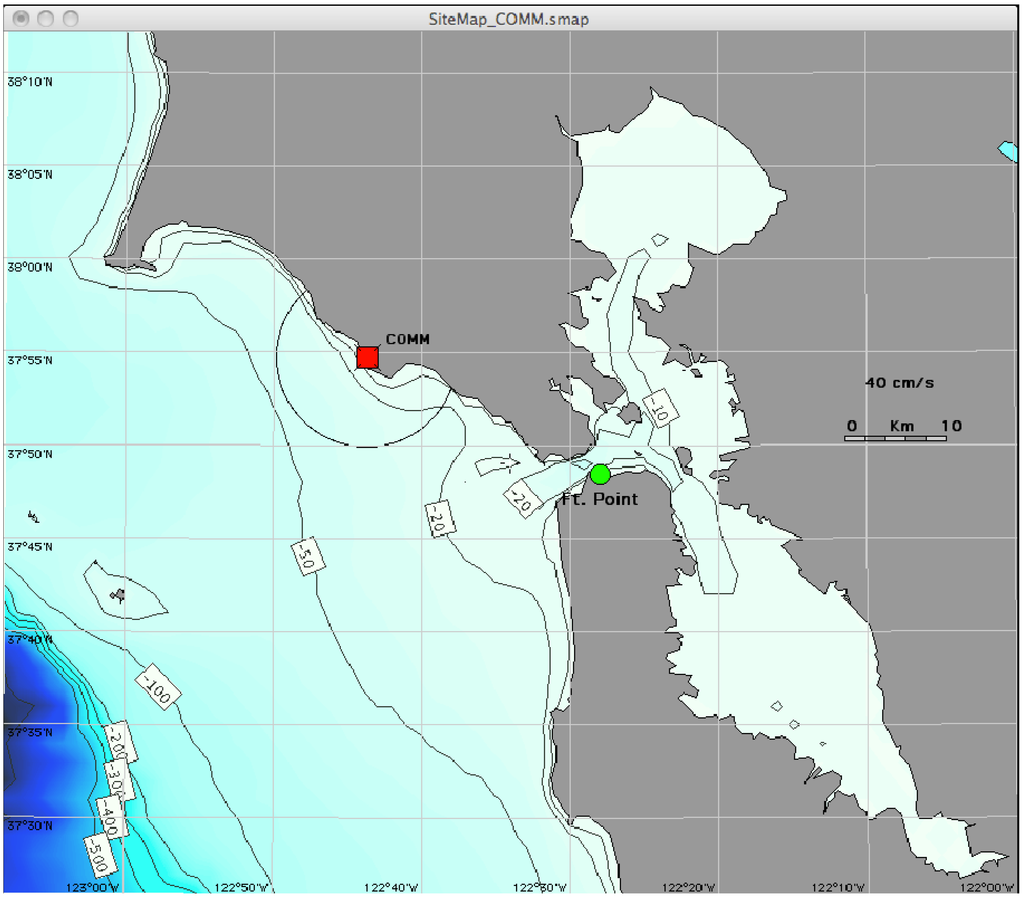
Figure 9.
The location of the radar near Bolinas, California, the tide gauge at Fort Point and the offshore bathymetry. Also marked is a circular radar range cell used in the centroid frequency analysis.
Figure 9.
The location of the radar near Bolinas, California, the tide gauge at Fort Point and the offshore bathymetry. Also marked is a circular radar range cell used in the centroid frequency analysis.

3.3. Tsunami Arrival Times as Seen by Radar and Tide Gauge
On the open ocean away from the coasts, the tsunami is a traveling shallow-water wave. The orbital velocity is a maximum at the wave crest; i.e., height and velocity are in phase. As the first crest approaches the coast, its velocity transports a volume of water shoreward like a breaking wave. At the beginning of this process, velocity may be high, but height only begins to increase. So height lags velocity. The wave runs up the shore until the velocity falls to zero and the height reaches a maximum; kinetic energy has been converted to potential energy at the boundary. Then the velocity reverses, causing a reflected wave motion to develop. Water is transported offshore and the water level at the shore decreases. If the tsunami wave were a pure sinusoid over time, height and velocity would be in quadrature at the coast, with the height lagging the velocity by a quarter cycle. Further offshore, the reflected and incoming waves combine to give local phase shifts and interference effects, with the details depending on the relative strengths of the incident and reflected waves.

Figure 10.
(a) Radial current velocity estimates with long-term trends removed, obtained from the frequency shift of the Bragg peak centroid frequency from the ideal Bragg frequency for three co-located radar antennas near Bolinas, California, (13 MHz transmitter frequency) plotted vs. time; (b) Time series of velocity components from the radar near Bolinas Radial velocities were resolved perpendicular to the shore, and averaged over bands 2 km wide parallel to the shore; (c) Simultaneous tide gauge water level measurements at Fort Point, at the mouth of San Francisco Bay, with long-term trends removed.
The arrival of the tsunami is signaled by the commencement of distinctive oscillations in the radar current velocity and in the tide gauge water level. Our data shows that the start of oscillations in velocity precedes that in water level. The delays have the following approximate values (a) 43 minutes: tide gauge at Hakodate vs. radar at Kinaoshi (Figure 4); (b) 12 minutes: tide-gauge at Pt. Reyes vs. radar at Bodega Marine Lab. (Figure 6); (c) 14 minutes: tide gauge at Crescent City vs. radar at Trinidad River (Figure 8); (d) 30 minutes: tide gauge at Ft. Point vs. radar near Bolinas (Figure 10). The delays can be explained as follows:
- (1).
- As for tidal flow, the velocity and height at the coast are typically in quadrature, implying a quarter cycle delay in the latter; i.e., 10 minutes delay for a 40-minute tsunami period. The coastal water level only begins to rise as the velocity increases to near its maximum, and does not reach its peak until some time later.
- (2).
- For cases (b) and (d), the tide gauge is further than the radar along the great circle path of the tsunami from Northern Japan; the resulting delay depends primarily on the details of the propagation through the shallow coastal waters.
- (3).
- The tsunami slows down markedly as it enters shallow water [1]. The tide gauges are on the shoreline, the radar measurements are in deeper water. For example, consider the bathymetry surrounding the Hokkaido radar and tide gauge shown in Figure 3. Tracing the tsunami path perpendicular to the depth contours, it can be seen that there is a more tortuous path for it to get to the tide gauge than to the radar. The tsunami is moving slowly as the water is very shallow over much of the path
4. Conclusions
We have described the first observations of a tsunami with coastal HF radars, using three different analysis methods to observe the tsunami signal, revealing its presence at different stages of the signal processing chain and demonstrating the expected current flows and velocity oscillations due to the tsunami: Method 1: Based on maps of total current velocity and water level as described in Section 3.1.1. This may be the most useful method for the study of computer modeling. It does require the tsunami to be observable in the common coverage area of at least two radars and thus requires extended shallow water as at Hokkaido (not the case for the California sites adjacent to a narrow continental shelf). Method 2: Based on analysis of radial current velocities from a single radar site averaged over bands approximately parallel to the depth contours as described in Section 3.1.2. This is the first step in observing the tsunami in localized offshore locations, the next being to use the actual bathymetry and the motion of the tsunami perpendicular to the depth contours. This may be the most useful method to provide warning of a tsunami approach, based on observation of velocity oscillations at distant ranges. Method 3: Based on estimating velocity from variations in the centroid frequency of the first-order Bragg spectral peak as described in Section 3.2. The resulting characteristic oscillations indicate that a tsunami is observable at the radar spectral level, before analysis to give radial and total current velocity vectors. The centroid velocity depends on both the current and wave field over the circular annulus of a radar range cell and thus has limited spatial resolution as the range increases.
While there is no doubt that tsunami signals have been observed in the data from Hokkaido and California, they were visible only a short time before impact on the shore. This is due to the short range of the Hokkaido radars and the narrow continental shelf off the western US coast. Nevertheless the results show promise for improved offshore detection. Using similar methods in ongoing studies, we can now provide accurate estimates of the observation/warning times for other regions, e.g., the US east coast, South East Asia and the west coast of India, where shallow-water bathymetry extends well offshore. HF radar installations at such locations will provide vital capability for the detection and measurement of the local intensity of deadly approaching tsunamis as well as detailed comparisons between observation and model predictions.
Further examination of the broad area data including comparisons with models is now possible and should lead to refinements of our understanding of tsunamis in coastal waters. These more in-depth studies of the complex tsunami phenomena occurring very close to the shore are left for the future, as are many others based on radar observations of tsunamis.
Acknowledgments
We are grateful to Bruce Nyden for collecting and processing radar and tide data, preparing the figures and providing editorial comments, and to James Isaacson for preparing the bathymetric displays. We thank Max Hubbard for his support with data collection and analysis, Kazuhiko Suguro and Yoshinori Namiki for providing data and coordinating with co-authors, Deedee Shideler and Marcel Losekoot for operating Bodega Marine Laboratory systems and for data management. We thank engineers at Aero Asahi Corporation for supporting system setup and data management in Japan. We also appreciate Japan Meteorological Agency for providing tide gauge data observed at Hakodate. This research was supported in part by the National Science Foundation, grant #ATM 0619139 to UC Davis and the WEST program, the State of California’s Coastal Conservancy, California Ocean Current Monitoring Program (http://www.cocmp.org/), the Sonoma County Water Agency, the NOAA IOOS Office, and the UC Davis Bodega Marine Laboratory.
References
- Barrick, D.E. A coastal radar system for tsunami warning. Remote Sens. Environ. 1979, 8, 353–358. [Google Scholar] [CrossRef]
- Lipa, B.J.; Barrick, D.E.; Bourg, J.; Nyden, B.L. HF radar detection of tsunamis. J. Oceanogr. 2006, 2, 705–716. [Google Scholar] [CrossRef]
- SeaSonde; Codar Ocean Sensors. Available online: http://www.codar.com/SeaSonde.shtml (accessed on 9 June 2011).
- Kaplan, D.M.; Largier, J.L.; Botsford, L.W. HF radar observations of surface circulation off Bodega Bay northern California, USA. J. Geophys. Res. 2005, 110, C10020. [Google Scholar] [CrossRef]
- Kaplan, D.M.; Largier, J.L. HF-radar-derived origin and destination of surface waters off Bodega Bay. Deep Sea Res. II 2006, 53, 2906–2930. [Google Scholar] [CrossRef]
- Kinsman, B. Water Waves; Prentice Hall: Upper Saddle River, NJ, USA, 1965. [Google Scholar]
- Karim, M.F.; Roy, G.D.; Ismail, A.I.; Meah, M.A. A shallow water model for computing tsunami along the West coast of peninsular Malaysia and Thailand using boundary-fitted curvilinear grids. Int. J. Tsunami Soc. 2007, 26, 21–41. [Google Scholar]
- Lipa, B.J.; Barrick, D.E. Least-squares methods for the extraction of surface currents from CODAR crossed-loop data: Application at ARSLOE. IEEE J. Ocean. Eng. 1983, OE-8, 226–253. [Google Scholar] [CrossRef]
© 2011 by the authors; licensee MDPI, Basel, Switzerland. This article is an open access article distributed under the terms and conditions of the Creative Commons Attribution license (http://creativecommons.org/licenses/by/3.0/).