1. Introduction
The Agriculture Camera (AgCam) is a two-band imaging system developed by the University of North Dakota for deployment on the International Space Station (ISS). Looking through a high-quality optical window on the ISS, AgCam will take images in red and near-infrared (NIR) wavelengths, with a ground sample distance of about 9 m. These bandpasses were chosen to select for vegetation response, in particular to enable generation of a Normalized Difference Vegetation Index (NDVI) value [
1]. Sponsored by NASA’s Education Office, the launch of AgCam via Space Shuttle Endeavour on November 14, 2008 was the culmination of a series of successful projects undertaken by over 50 undergraduate and graduate students at the University. To keep costs low, for selected components AgCam used commercial-off-the-shelf (COTS) products, in particular those that were challenging to address within a student-led design team. Electro-optical components of AgCam include an f/2.8 Mimaya lens, a beam splitter, and two digital scan line cameras (Dalsa CL-P4-8192) each with a CCD array of 6,144 cells [
2]. AgCam is capable of pointing in a cross-track direction of up to ±30°, enabling multiple revisits of a target during a short time period. Despite its use of low cost COTS components, AgCam is intended to be used for scientific and practical applications in precision agriculture and natural resource management; therefore precise determination of its electronic, optical, spectral and radiometric characteristics is needed.
In collaboration with the Airborne Remote Sensing Laboratory at the NASA Ames Research Center, we fully characterized the electro-optical components of the AgCam, producing these primary measurement sets: (1) bandpass spectral responsivity; (2) raw output in digital number throughout the dynamic range of the sensor, corresponding to known radiometric input levels; and (3) digital number output response to a Lambertian illumination at different integration times.
These characterizations identified three major sources of artifacts affecting the electro-optical performance of the AgCam: vignette effect; non-uniform quantum efficiency among various CCD cells; and dark current. Vignette effect refers to the reduction of illumination from the center of an image towards the edge, which results from a combination of increasing path length and incident angle, and decreasing solid angle due to blockage by the aperture, as a ray moving from the center to the edges of a CCD array [
3]. Theoretically, for an optical lens system the vignette effect pattern follows cos
4α, where α is the angle between a ray and the camera optical axis. But for most imaging systems, the vignette effect is much more complex and is typically studied with raying tracing and modeled empirically using polynomial functions or hyperbolic cosine functions [
4,
5,
6,
7,
8,
9]. Because no two CCD detectors are the same, their differences in non-uniform quantum efficiency lead to differences in photo-electric responsivity. Dark current is associated with bias current or voltage that is inherent for the electronic components [
10] and is expected to vary with each detector.
Often both vignette effect and non-uniform quantum efficiency effects are corrected at the same time such that a flat field is reproduced under a uniform illumination [
11]. Seibert
et al. [
12] acquired multiple images of a uniform light field over a range of exposure times, and derived correction coefficients statistically from these images. The advantage of their method is that the random noises can be suppressed statistically. Because relatively high noise levels were expected from the COTS components from which AgCam was built, we will use Seibert
et al.’s method to derive the correction coefficient for vignette effect and quantum efficiency. Most applications of AgCam require the use of radiometric quantity instead of digital number, therefore we need to separate vignette effect and quantum efficiency from each other so that radiance can be derived for every CCD cells.
2. AgCam System
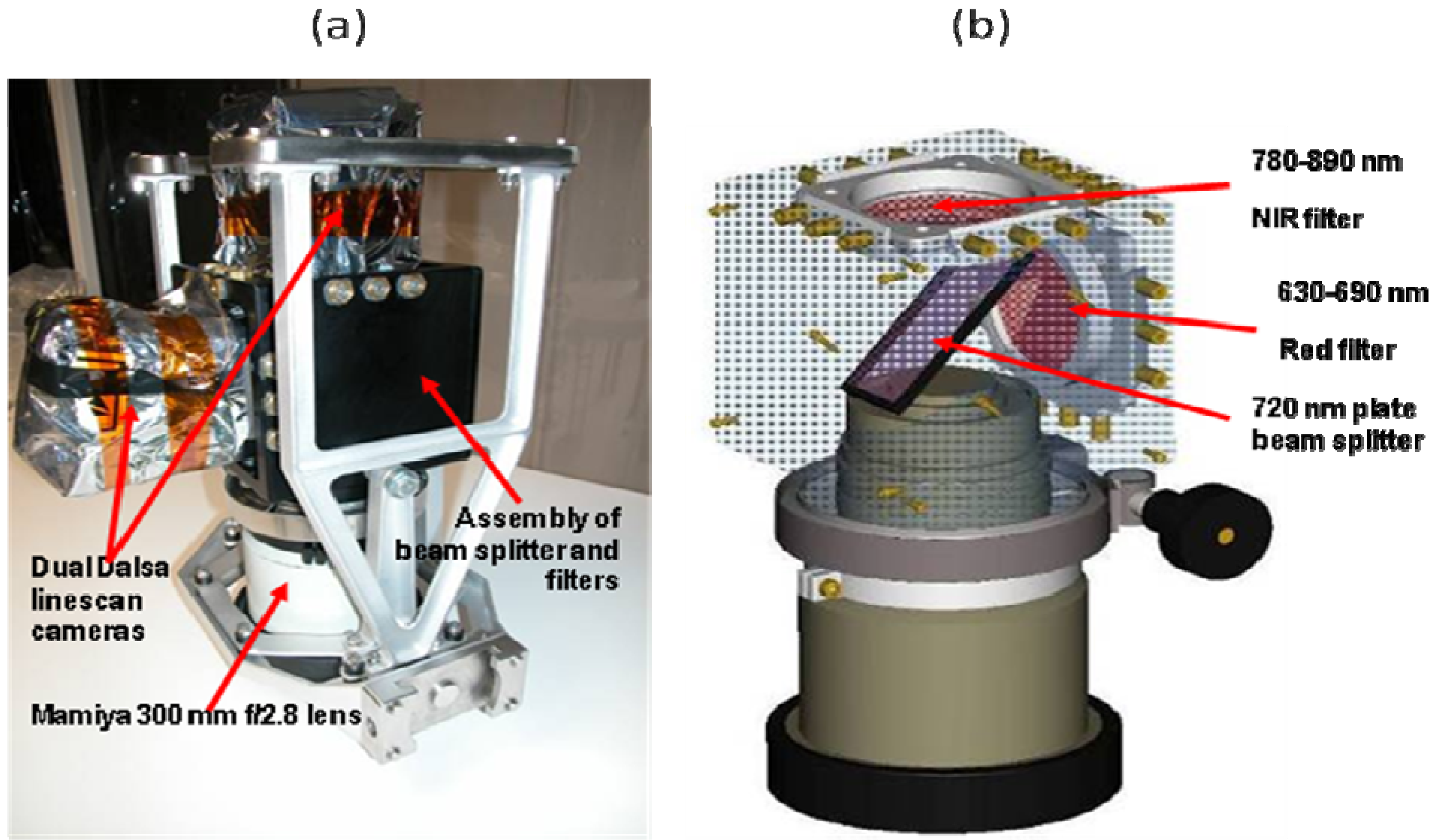
Figure 1 illustrates the AgCam sensor electro-optical components. An f/2.8 medium format lens with 300 mm focal length manufactured by Mamiya was modified to permanently set aperture at maximum and focus at infinity, and to remove structure such that an optical beam splitter could be situated within the back focal length distance of the final lens element. Coatings on the 2 mm glass plate beam splitter element separate the incoming radiation into a reflected beam with wavelengths <720 nm and a transmitted beam with wavelengths >720 nm. The two beams are further filtered with a red filter of bandpass 630–690 nm and a NIR filter of bandpass 780–890 nm, respectively, before reaching the cameras. To correct for astigmatic effects inherently produced by rays converging across the relatively thick inclined plate beam splitter, a cylindrical lens (not shown) was inserted between the beam splitter and the NIR filter. Lens modification, beam splitter and bandpass filter manufacture, and optical system integration was performed by Coastal Optical, Inc. (West Palm Beach, FL, USA).
Figure 1.
Electro-optical components of AgCam. (a) components integrated in vibration isolation and absorption frame, and (b) computer-aided-design model of internal optical beamsplitter and trim filters.
Figure 1.
Electro-optical components of AgCam. (a) components integrated in vibration isolation and absorption frame, and (b) computer-aided-design model of internal optical beamsplitter and trim filters.
The sensor on each Dalsa camera consists of 8,192 7 × 7 micron CCD detectors in a linear array, only the center 6,144 of which are read by the AgCam’s electronic system, producing linescan imagery when in motion. Gain settings are internally fixed, and imaging control is limited to user-specified integration time and line period. Preliminary tests and analysis indicated sensor dynamic range would be insufficient to capture the top-of-atmosphere radiance expected from typical vegetation targets while maintaining comparable integration times across both channels. Reducing internal gain settings in the NIR camera and increasing them in the Red camera compensated for dynamic range limitations, though this also resulted in increased noise in the red channel.
The ISS orbits at 51.6 degree inclination, with an altitude that varies between 350 and 420 km. Orbital speed varies accordingly; a nominal velocity of 7,220 m/s at 400 km altitude yields a line period of 1.293 ms. Integration time for a typical vegetation target is expected to be about 0.2 ms. Mounted inside the ISS, AgCam will observe Earth’s surface through the U.S. Laboratory Destiny Science Window [
13]. Pre-flight optical transmittance of the window was measured by NASA; transmittance in the red and NIR AgCam channels is estimated to be 98.0% and 93.4%, respectively, with negligible variation as a function of look angle obliqueness [
13].
3. Laboratory Calibration
In addition to performing specialized sensor development and operation, the Airborne Remote Sensing Laboratory (ARSL) at the NASA Ames Research Center maintains and operates a high quality laboratory for accurate sensor characterization and calibration. Three calibration instruments at the ARSL were used to characterize the AgCam sensor:
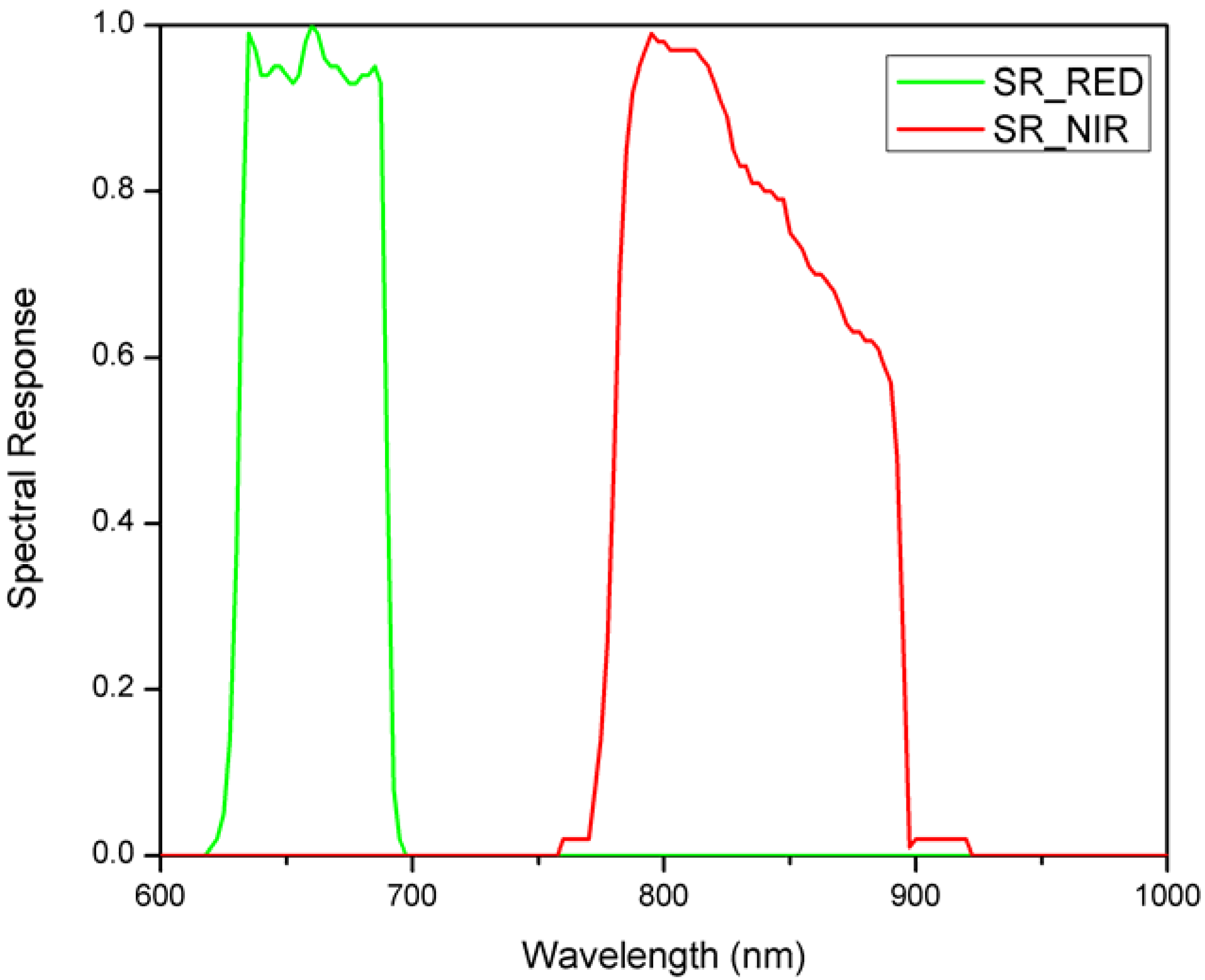
(1) Spectral characterization was performed using an Oriel 7345 tunable narrowband monochrometer, with associated changeable reciprocal linear dispersion gratings, off-axis parabolic mirror collimator, and turning mirror with a surface accuracy <λ/4, where λ is the wavelength. The FWHM for the collimated light is 1.5 nm. A full spectrum scan was first performed to validate the bandpass of the trim filters. Next, spectral response for each camera was determined every 3 nm, and repeated for 5 incident angles of −4, −2, 0, 2, and 4° to evaluate the angular variations within the field of view of AgCam (~8°). Before and after each measurement, reference spectra were recorded using a calibrated silicon photodiode to monitor the stability of the light source. The spectral response determined for the AgCam showed little angular variations and the nadir one is shown in
Figure 2.
Figure 2.
AgCam spectral response.
Figure 2.
AgCam spectral response.
(2) Radiometric characterization was performed using a 30 inch diameter Archi 12-bulb integrating sphere calibrated to an FEL lamp traceable to the U.S. National Institute of Standards and Technology (NIST) standard of spectral irradiance. During calibration, the integration time for both cameras was set at 100 µs. The light bulbs were turned on successively and the camera took images looking into the integrating sphere cavity at each level until saturation, which occurred at 6 bulb levels for the NIR channel and 5 for the red channel. The radiance at each bulb level was calculated by convolving AgCam spectral response (determined above) with the irradiance spectra of the light bulbs that were known
a priori [
14].
(3) Uniform target imagery was obtained from a flat-field uniform source, which uses diffuse glass emission plate with multiple reflective internal baffles between the output plate and an adjustable stable bulb source. The exiting light field is within 1% Lambertian for angles up to 30 degrees. Placement of the AgCam sensor within a few centimeters of the output diffuser further improved quality of the exiting light field, as near-field de-focus effects averaged any residual source variations from dust or other minor source defects. The light intensity is fixed during the experiment and five sets of images of 1-second duration were taken at integration time of 100, 200, 300, 400, and 500 μs, respectively; line period was set to 1,400 μs.
Images corresponding to the dark current were also obtained at each integration time by capping the camera’s lens.
4. The Modeled AgCam System
The signal recorded by a CCD detector,
DN(
i) (
i = 1–6,144), looking at a target with emitting radiance
L(
i), can be modeled as [
7,
15,
16,
17,
18,
19]:
where:
- -
DN(i) is the raw output as a digital number between 0~255 (8 bits digitization);
- -
DN0(i) is the digital number dark current offset of CCD cells, a threshold below which no output will be triggered even there is impinging light;
- -
VE(i) represents the vignette effect;
- -
QE(i) represents quantum efficiency coefficients, which determine the conversion of digital number values into radiant energy;
- -
t is the integration time (unit is µs) and L(i)t would be the total energy received by the CCD cell (i) during the acquisition of an image.
It is clear from Equation (1) that to derive the input radiance
L(
i), three sets of parameters of
DN0(
i),
VE(
i) and
QE(
i) for each CCD cell need to be determined. During the calibration, the incident light field is uniform, (denoted as
L0), and Equation 1 becomes:
Because of inter-CCD detector variations in DN0(i), VE(i) and QE(i), we expect the digital number values will vary for different CCD cells even under uniform illumination. The purpose of radiometric calibration that we have conducted was to derive parameters DN0(i), VE(i) and QE(i), so that an incident radiation field for an arbitrary operational image can be determined.
5. Calibration Analysis and Results
For the same CCD cell during one calibration procedure, we expect the response to be stable. After removal of known synchronous electronic noise effects, analysis of all the uniform target images in the NIR band showed that the response of any one CCD detector was relatively constant with a standard deviation less than 1 digital number. For the noisier red band, standard deviation was less than two digital numbers. Therefore, all the images were averaged along the direction of scan (or time), with each image reduced to a vector corresponding to the mean state of response of the CCD array. Because the analysis approach for the two bands is the same, and the relative degree of correction achieved for the two bands are comparable, we will present the results for the NIR band only unless indicated otherwise.
5.1. Dark Current Offset
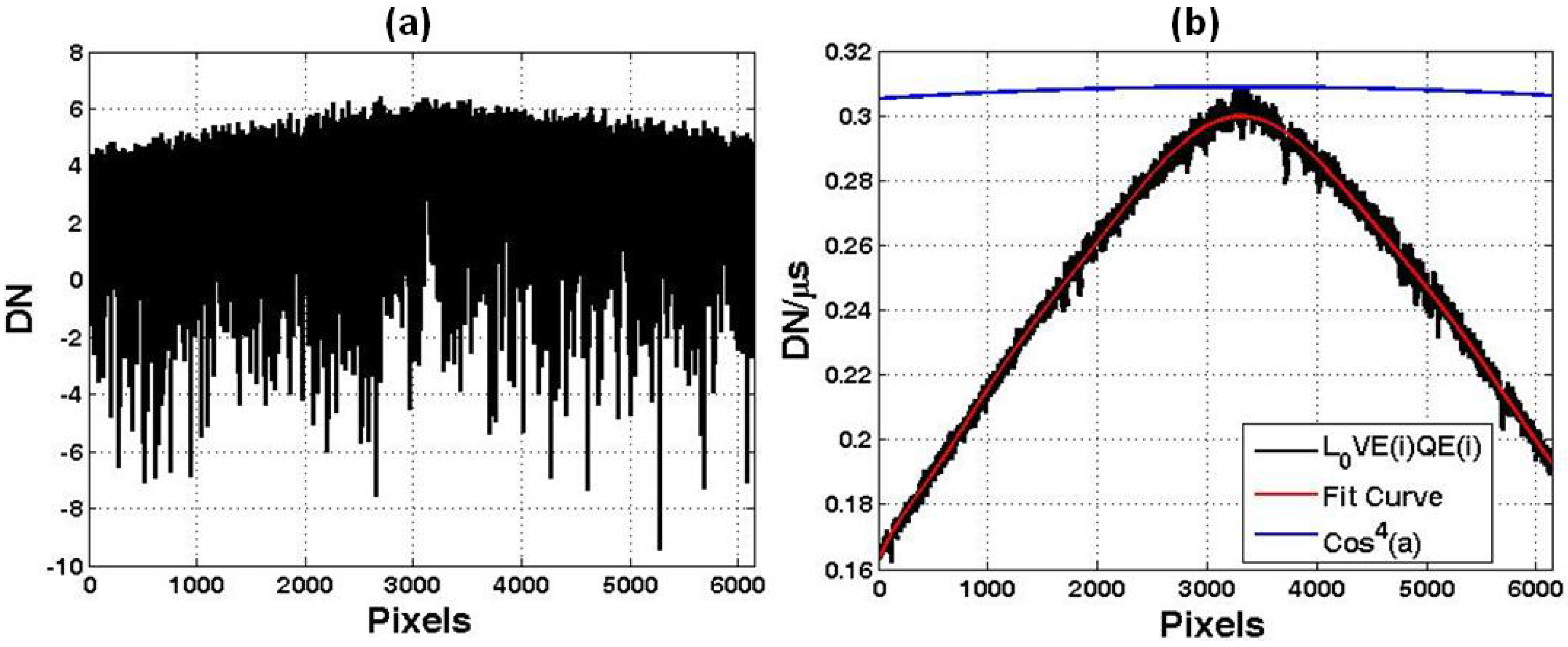
As described, five sets of images were taken of a uniform target at five integration times, specifically 100, 200, 300, 400, and 500 µs. This leads to five set of equations of Equation (2). The terms
DN0(
i) and
L0VE(
i)
QE(
i) can be derived by applying a least squares regression on these five images, and the results are shown in
Figure 3 [(a) for
DN0(
i) and (b) for
L0VE(
i)
QE(
i)]. For a perfect CCD detector, the
DN0 would be zero; no output would be generated when there is no incident light.
Figure 3 (a) shows that
DN0(
i) varies roughly between −9 and 7 digital counts. The mean of
DN0(
i) determined using this least-square method is about 3.5. The mean value of
DN0(
i) measured when the images were taken with the lens capped was also approximately 3.5, an independent validation.
Figure 3.
The terms of Equation 2 determined from the Least Square analysis of the 5 sets of images of a uniform target at different integration time, (a) DN0(i) and (b) L0VE(i) QE(i). The blue curve in (b) is cos4α and the red curve polynomial fit at 9th order.
Figure 3.
The terms of Equation 2 determined from the Least Square analysis of the 5 sets of images of a uniform target at different integration time, (a) DN0(i) and (b) L0VE(i) QE(i). The blue curve in (b) is cos4α and the red curve polynomial fit at 9th order.
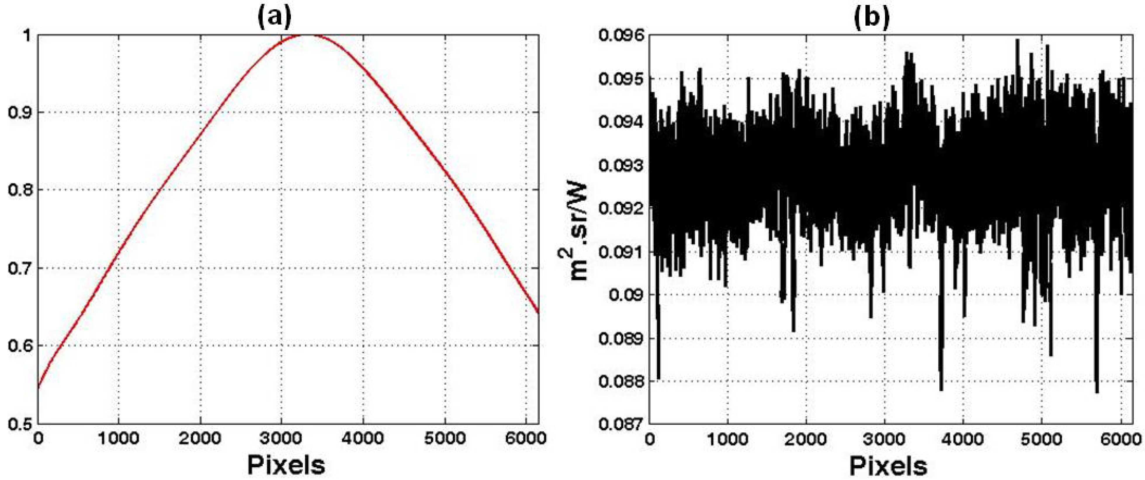
5.2. Vignetting Effect Correction
Shown in
Figure 3(b), the term
L0VE(
i)
QE(
i) of Equation (2) exhibits two notable features: a rapid dropping in values towards the edges presumably due to the vignette effect and a seemingly random variation overlaid on the vignette effect trend. The latter random variation is due to the non-uniform quantum efficiency among CCD detectors. The blue curve in
Figure 1(b) is the vignette effect modeled by the cos
4α law using the AgCam optical parameters. The large discrepancy between the actual and the modeled vignette effect, 55%
vs. 1.2% drop at the edges, suggests the AgCam optical system is more complex than the simple vignette model can predict. This complexity is certainly due to the optical components of the system in addition to the Mamiya lens, including the beam splitter, the filters, and the corrective cylindrical lens.
Figure 4.
(a) Vignette effect correction coefficients—VE(i). (b) Quantum efficiency calibration coefficient—QE(i).
Figure 4.
(a) Vignette effect correction coefficients—VE(i). (b) Quantum efficiency calibration coefficient—QE(i).
The vignette effect is expected to vary smoothly from the center to the edges because it is caused by optical components in the AgCam system, while the quantum efficiency factor may vary randomly among CCD cells due to inherent cell-to-cell variations introduced during the manufacturing process. To separate the two effects, we applied a polynomial fitting to
L0VE(
i)
QE(
i). After testing with different orders between two to 12, we chose the ones that gave the minimal residual variances: nine for the NIR and six for the Red. The polynomial curve is shown in
Figure 3(b) as a red curve. Assuming there is no vignette effect at the principal optical axis, namely,
VE(
i0) = 1, we derived the
VE(
i) [shown in
Figure 4(a)] by normalizing the red curve in
Figure 3(b) with its maximum, which is located at CCD cell No. 3304. The principal optical axis is thus not aligned at the center of the CCD array (
i.e., No. 3072). This misalignment, however, will not affect the calibration or the quality of imaging. The ratio of the two curves,
L0VE(
i)
QE(
i) [the black line in
Figure 3(b)] to that of
VE(
i) [the red line in
Figure 4 (a)], gives
L0QE(
i); this will be used later to derive
QE(
i).
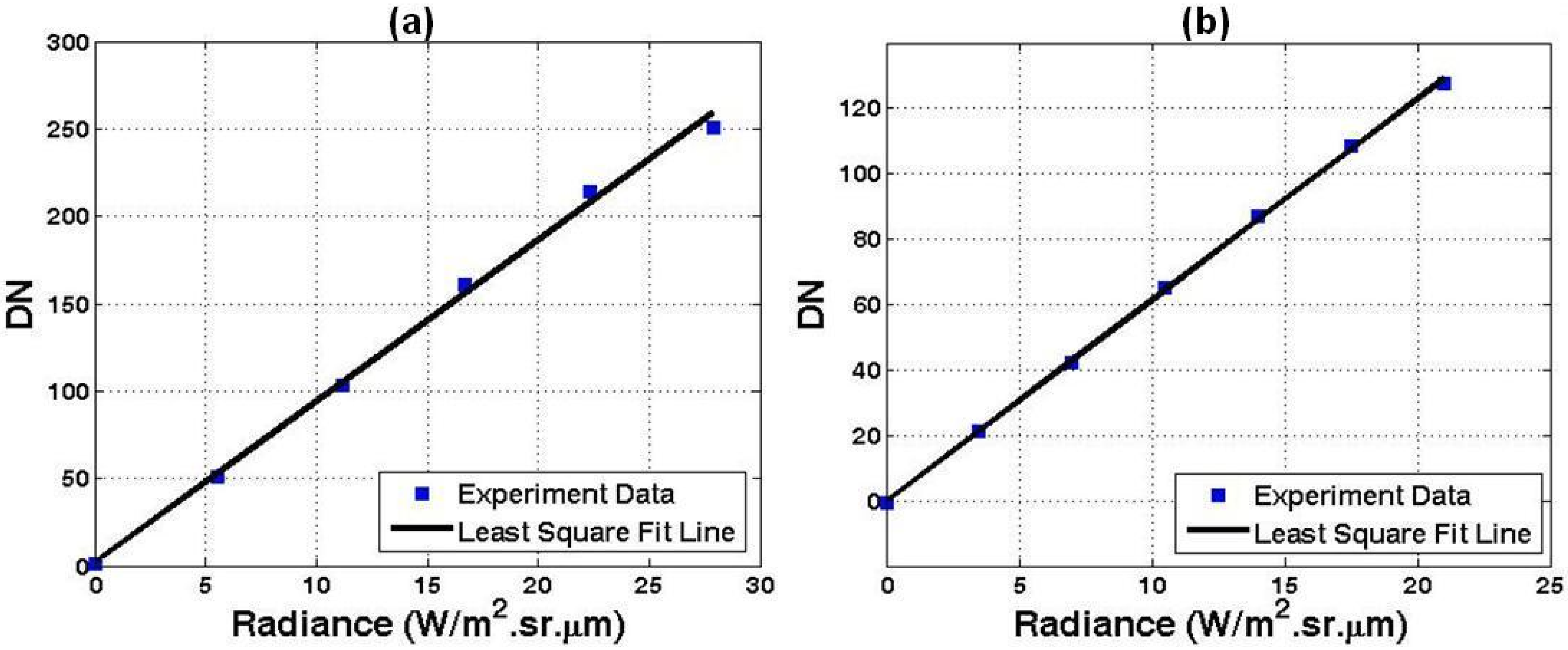
5.3. Quantum Efficiency Calibration
During the radiometric calibration, six images of the integrating sphere cavity were taken, with each corresponding to the number of light bulbs turned on. Correcting for digital number offset as described above and following Equation (1), the resultant digital number at the principal axis can be modeled as:
where
- -
i0 denotes the location of the principal optical axis. Also we have assumed VE(i0) = 1.
- -
the number of 100 in Equation (3) is the integration time which was fixed at 100 µs during the radiometric calibration.
The variations of digital number with
L are shown in
Figure 5(a) for the NIR band and (b) for the red band, respectively. The red band saturated at the 6th bulb level, so the value was not used. The slope of the calibration curve in
Figure 5(a) is the quantum efficiency coefficient [
QE(
i0)] at the principal axis. With this and the curves shown in
Figure 3(b) and
Figure 4(a), straightforward derivation produces
QE(
i) for the entire CCD array, shown in
Figure 4(b).
Figure 5.
AgCam Radiance Calibration Curve (100 μs). (a) NIR Band; (b) RED Band.
Figure 5.
AgCam Radiance Calibration Curve (100 μs). (a) NIR Band; (b) RED Band.
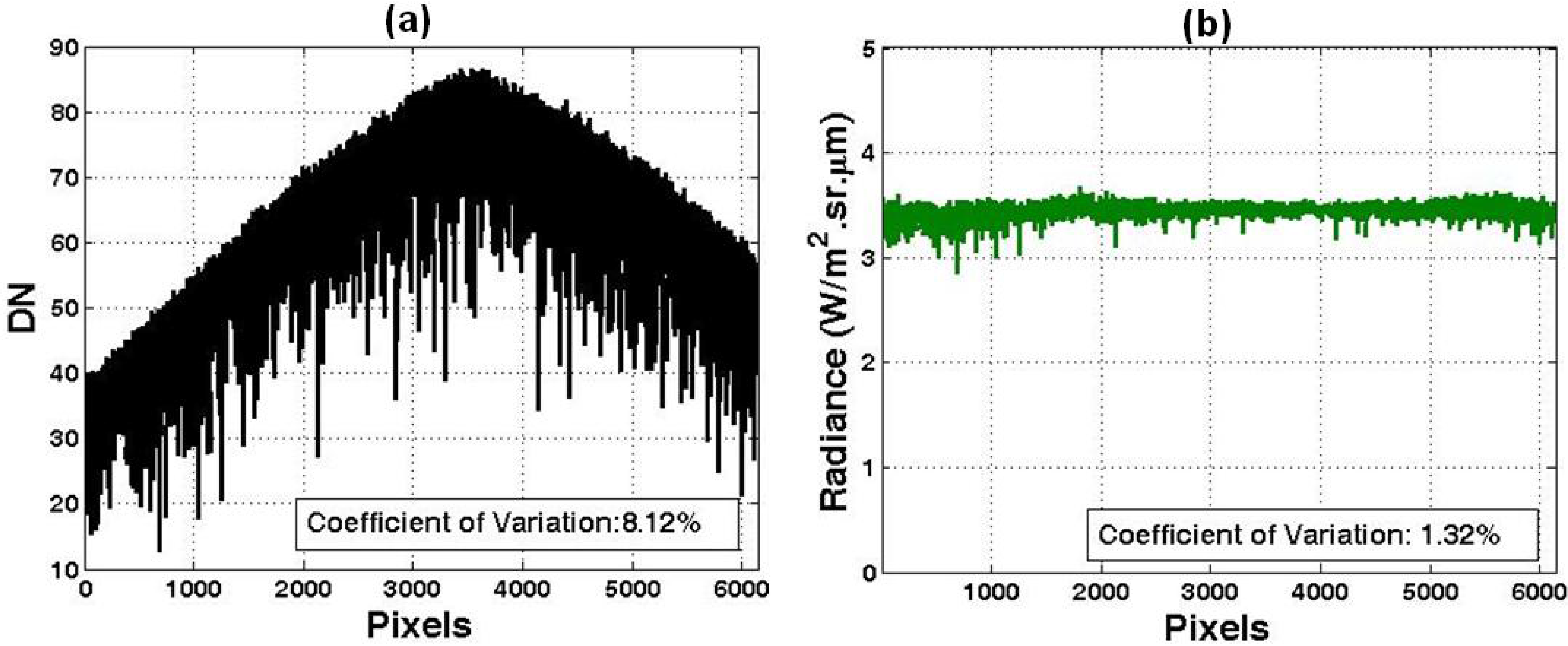
5.4. Calibration Results
Now we can correct AgCam images radiometrically with the parameters determined for
DN0(i),
VE(
i), and
QE(
i), respectively. The results for the NIR band at 200 μs and RED band at 300 μs. are shown in
Figure 6 and
Figure 7, respectively [(a) for uncorrected and (b) for corrected images].
For the NIR band, the correction has largely reproduced the known uniformity of the incident light field. The Red band (
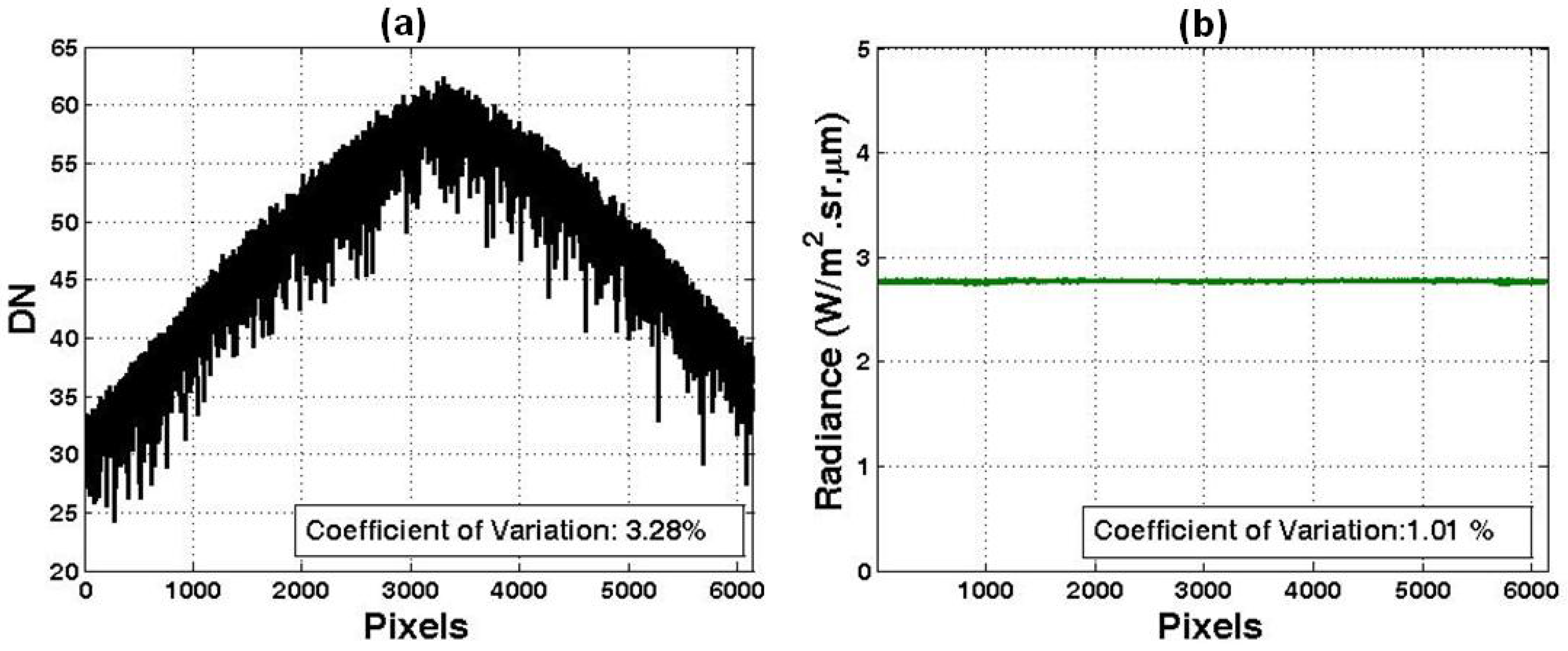
Figure 7) is also substantially corrected, though with more residual absolute variance than in the NIR channel. This is assumed to be due to the higher level of noise introduced by the higher gain setting of the red channel, as described in
Section 2. Application of the correction algorithm to the original uniform target images significantly reduced artifacts within each image. After removing the vignette effect, coefficient of variation due to random quantum efficiency effect was reduced from 3.28% to 1.01% for the NIR band, from 8.12% to 1.32% for the red band, improving 69.2% and 83.7%, respectively.
Figure 6.
Results of 200μs NIR. (a) Uncorrected data; (b) Radiance of calibrated data. The coefficient of variation for (a) was estimated after the vignette effect was corrected.
Figure 6.
Results of 200μs NIR. (a) Uncorrected data; (b) Radiance of calibrated data. The coefficient of variation for (a) was estimated after the vignette effect was corrected.
Figure 7.
Same as
Figure 6 but for the Red band with an integration time of 300 μs.
Figure 7.
Same as
Figure 6 but for the Red band with an integration time of 300 μs.
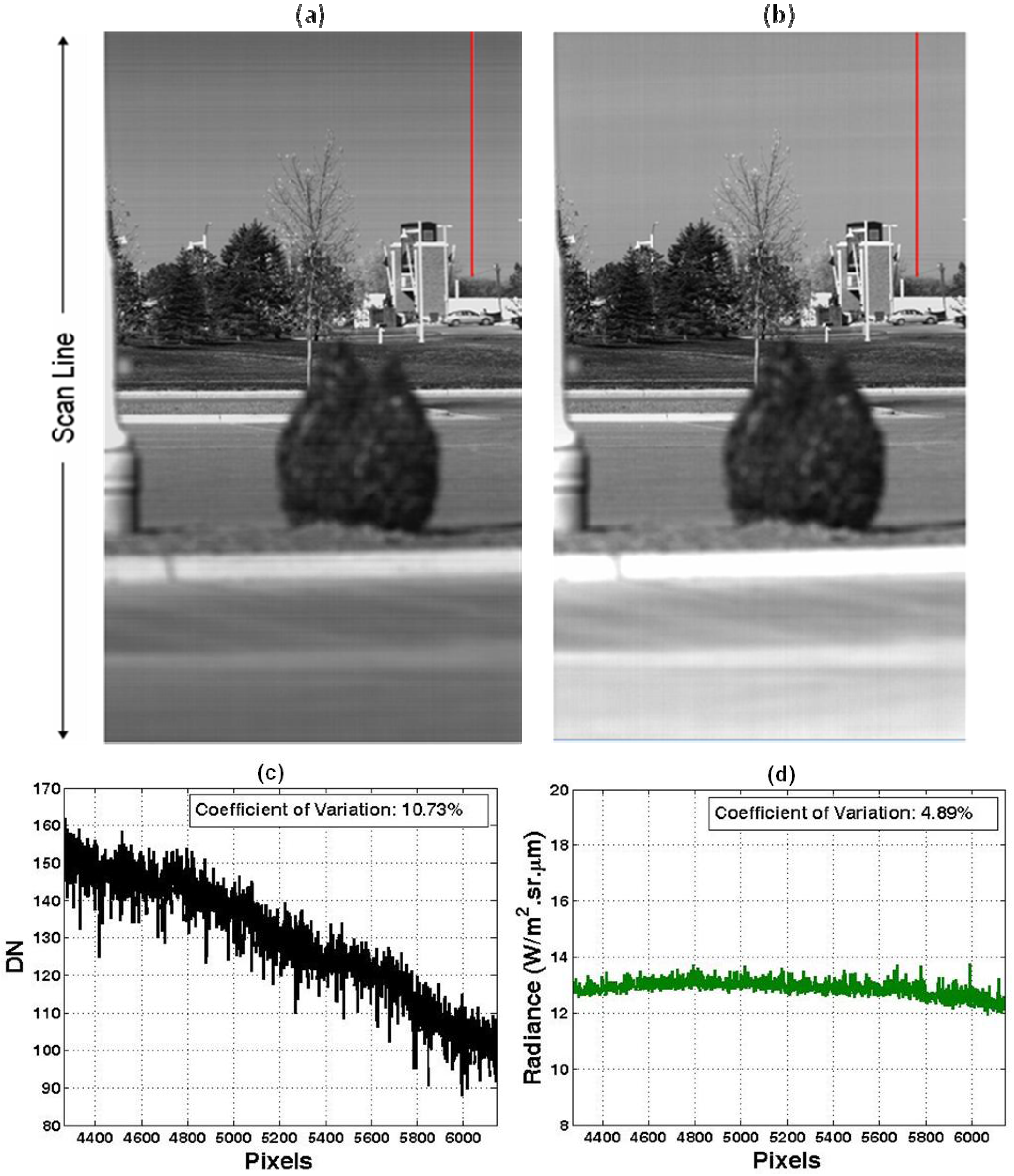
6. Applications to AgCam Imagery
The described calibration algorithms have been applied to test imagery collected using the AgCam sensor during ground-based testing. As a linescan imager, AgCam requires motion between sensor and target to generate images. An Ideal Aerosmith 1291BR Single Axis Positioning and Rate Table System was used to create relative motion comparable to that which will be observed on orbit. The AgCam sensor was placed on the rate table platform with its CCD array oriented vertically; then rotated clockwise horizontally, sweeping the CCD array from left to right across the landscape. Imagery examples are shown in
Figure 8 and
Figure 9; with the lens at infinity focus, near-field effects blur objects that are less than ~200 meters distant.
Figure 8(a) was acquired October 5, 2006 on the UND campus, with integration time at 200 µs;
Figure 9(a) was acquired August 1, 2006 at Coastal Optical Inc. (West Palm Beach, FL, USA) with integration time set at 300 µs.
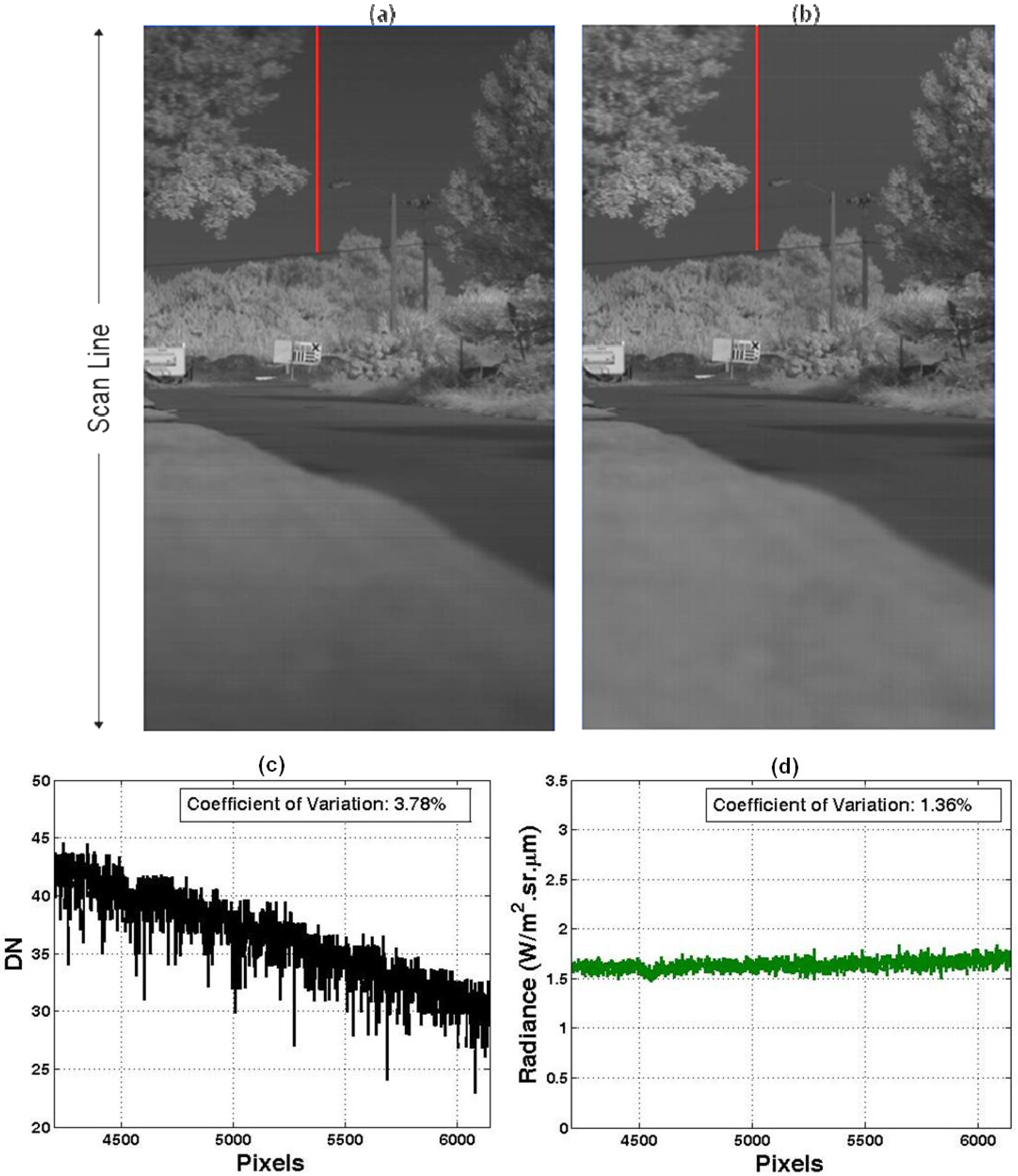
Figure 8.
Results of calibrated AgCam image (RED, 200 μs). Data was acquired October 5th, 2006 at Grand Forks, ND. (a) Uncorrected AgCam raw image; (b) Radiometrically corrected images; (c) A selected scan line from AgCam raw image (Red line in (a)); (d) The same scan line from radiometrically corrected images (Red line in (b)). The coefficient of variation for (c) was estimated after the vignette effect was corrected.
Figure 9.
Same as
Figure 8 but for AgCam image (NIR, 300 μs), acquired August 1st, 2006 at West Palm Beach, FL.
Figure 9.
Same as
Figure 8 but for AgCam image (NIR, 300 μs), acquired August 1st, 2006 at West Palm Beach, FL.
Calibration algorithms were applied to these two image sets. The radiometrically corrected images are shown in
Figure 8(b) and
Figure 9(b) respectively. For both of the experiments, a portion of sky with roughly the same illumination was captured. A sample of the sky light distribution along the red line is shown in
Figure 8(c) and
Figure 9(c) respectively. Both vignette and non-uniform quantum efficiency effects are apparent in the raw images, with digital number values decreasing towards the edge, and exhibiting large pixel-to-pixel variations. The radiometric correction applied significantly removed both effects, resulting a relatively uniform distribution of skylight as expected.
7. Conclusions
The AgCam sensor was designed in an academic environment using low-cost COTS components, and will collect remotely sensed imagery of the Earth in two spectral bands, red and near infrared. Because of its use of COTS products, the raw AgCam images exhibit significant artifacts due to vignetting and non-uniform quantum efficiency effects. By separating these effects and addressing them independently, each could be minimized. Precise radiometric calibration of the system enabled three calibration parameters to be derived; vignette effect, and quantum offset and efficiency for the CCD array. In the AgCam red channel, a higher fixed internal gain setting appears to result in a higher range of values for quantum offset and CCD efficiency, and subsequent greater uncertainty in calibration measurements. Nonetheless, application of the described calibration method resulted in a significant degree of correction for both bands, albeit with higher absolute residual errors in the red channel. While residual errors may be a limiting factor for some applications, applying the described calibration parameters will produce much higher quality operational images than would otherwise be available, with units of quantitative radiant field, thus enabling them to be used in a variety of scientific and applied applications.
