1. Introduction
The biggest advances in forest inventory technology in recent years have been in applications based on airborne laser scanning (ALS). The two main approaches in deriving forest information from small-footprint ALS data have been those based on laser canopy height distribution (area-based method, [
1]) and individual tree detection [
2]. ALS is as accurate as traditional ocular field measurements in estimating the stand mean volume (V) at plot level with area-based inventory methods (e.g., [
3,
4]) or via single-tree characteristics (e.g., [
5,
6,
7]). Area-based laser scanning is more cost-efficient, due to its sparser pulse density requirements. Furthermore, tree-level estimation is computationally heavier; thus in large-area inventories the area-based approach can, at least currently, be considered more feasible. ALS is carried out at relatively low altitudes, which consequently makes it relatively expensive per area unit. Other remotely sensed data will still be needed, especially when updated information is required e.g.,several times per year. Of special interest are inexpensive images with favourable temporal resolution that can be utilized in multiphase sampling and change detection in addition to the ALS measurements.
A major advantage of radar images, compared with optical region satellite images, has been their ready availability (temporal resolution) under all imaging conditions. This makes radar imaging, especially the Synthetic Aperture Radar (SAR) carried by satellites, an intriguing option in developing methods for operational inventory of forest resources.
Most commonly, the amplitude information of SAR backscattering is exploited in the estimation of forest parameters. For example, Le Toan
et al. [
8] used an airborne multifrequency SAR system for demonstrating the capability of SAR images in forest biomass retrieval and concluded that the cross-polarization channel of the long wavelengths (L and P bands) yielded the best sensitivities. Later, promising results (with presumably enhanced estimation accuracies) were achieved, using SRTM (Shuttle Radar Topographic Mission) SAR interferometry [
9], interferometric coherence [
10], polarimetric SAR interferometry [
11], and fusion of SAR with airborne laser scanning (ALS) [
12]. The range measurements of ALS provide very accurate geometric information on forests. The main advantage of SAR, especially in the satellite-borne system, is the very frequent imaging capability in comparison to optical satellite images, aerial imagery and ALS.
SAR measurements experienced a breakthrough similar to that in the ALS method, when in the early 2000s satellite radar imagery with spatial resolutions as high as 1–3 m (single-polarization imaging) were developed. In addition to the improved spatial resolution, the central improvements in the new SAR satellite images have been their ability to utilize interferometry and polarimetry. In combining data from several satellite types, information from different wavelength areas can be obtained. These factors should improve the estimation accuracies in forest applications, compared with previous instrument generations.
Rauste
et al. [
13] reported that the estimation of growing stock volume is slightly more accurate with the full-polarimetric, high-resolution Advanced Land Observing Satellite (ALOS) radar images than with the earlier Japanese Earth Resources Satellite 1 (JERS-1), but the estimates still saturate at 150 m
3/ha. An airborne sensor, the Experimental Synthetic Aperture Radar (E-SAR), owned by the German Aerospace Centre (DLR), has been used to simulate the results obtainable with the TerraSAR-X. Holopainen
et al. [
14] compared E-SAR, Landsat Enhanced Thematic Mapper (ETM) and aerial photographs in estimation of plot-level forest variables and reported relative root-mean-squared-errors (RMSEs) for E-SAR of 45%, 29%, 28% and 38% for Vol (m
3/ha), mean diameter (D
g; cm) , mean height (H
g; m) and basal area (BA; m
2/ha), respectively. In combining E-SAR with aerial photographs, the relative RMSEs for the same variables were 38%, 26%, 23% and 33%. Rauste
et al. [
15], studied ALOS and TerraSAR-X data for mapping biomass in boreal forest zone, Finland. According to their results ALOS data performed better than TerraSAR-X data in biomass estimation. The phase of the HH-VV cross-coherence produced the highest biomass correlations among the TerraSAR-X features.
Holopainen
et al. [
16] investigated the theoretical benefit of using tree species-specific inventory data instead of stand-level mean data in forest-planning simulations. The results showed that the use of tree species stratum data in forest-planning simulations is highly relevant from the viewpoint of both the development of stand characteristics and the timing of logging operations. The significance of the stratumwise input data culminated in the functioning of the specieswise growth models at different stages of stand development.
While ALS data with very accurate height readings and consequent three-dimensional (3D) profiles of the stand are a great improvement over the traditional optical area sensors used in forest remote-sensing applications, there have been problems in tree species recognition and thus also species-specific estimates. In respect to area-based ALS interpretation, species stratum level characteristics are estimated at a considerably lower accuracy level than stand level mean characteristics. The relative RMSE of stratum level characteristic interpretation has been reported to range from 25% to 80% [
17,
18,
19]. Estimation accuracies can typically be improved with a combination of data sources with complementary properties. In the case of ALS data, combination with aerial photograph-based features has improved the species-specific results [e.g.,
20].
The objective of the study was to compare the accuracy of low-pulse ALS, high-resolution noninterferometric TerraSAR-X radar data and their combined feature set in the estimation of forest variables at the plot level. Genetic algorithms (GAs) were used to reduce the dimensions of the large feature sets; however, the original feature sets were also used for benchmarking results. The estimation was carried out with the nonparametric k-nearest neigbour (k-NN) algorithm. The forest variables estimated included mean volume (Vol), basal area (BA), mean height (Hg), mean diameter (Dg) and tree species-specific mean volumes for Scots pine (VolP), Norway spruce (VolS) and deciduous tree species (VolD).
2. Methods
2.1. Study Area and Field Data
The study area is located in the vicinity of Espoo, Finland (24°30’E and 60°18’N). The research material consisted of 124 tree level measured fixed-radius (7.98 m) plots. Field measurement data from these plots were collected in 2007 and 2008. The plots were located with ALS-based tree maps and the Global Positioning System (GPS). The following variables were measured of trees having a diameter-at-breast height (dbh) of over 5 cm: location, tree species and dbh. Tree heights were measured from 46 plots and the height model was then formulated. The volumes were calculated with standard Finnish models [
21]. Plot-level data were obtained by summing the tree data. Stand characteristics according to the field measurements are presented in
Table 1.
Table 1.
Mean, range and standard deviation of the stand characteristics (n = 124).
Table 1.
Mean, range and standard deviation of the stand characteristics (n = 124).
| | Mean | Min | Max | Std |
|---|
| Volume (Vol) | 196.3 | 9.1 | 541.3 | 113.6 |
| Basal area (Ba) | 24.5 | 1.6 | 59.5 | 11.2 |
| Height (Hg) | 17.2 | 6.1 | 24.2 | 3.5 |
| Diameter (Dg) | 26.6 | 8.4 | 41.0 | 6.7 |
| Volume, pine (VolP) | 58.7 | 0.0 | 287.5 | 75.1 |
| Volume, spruce (VolS) | 83.5 | 0.0 | 450.1 | 106.5 |
| Volume, deciduous (VolD) | 54.1 | 0.0 | 488.4 | 76.5 |
2.2. Acquisition and Processing of ALS Data
The ALS data were acquired on 14 May 2006 with an Optech3100 laser scanner. The flying altitude was 1,000 m. The density of the returned pulses within the field plots was approximately 4 points/m2. The ALS data were first classified into ground and nonground points. A digital terrain model (DTM) was then developed, using classified ground points and laser heights above ground (normalized height or canopy height) were calculated by subtracting the ground elevation from the laser measurements. Canopy heights close to zero were considered as ground returns and those greater than 2 m as vegetation returns. The data intermediate between them were considered as returns from ground vegetation or bushes. Only vegetation returns were used for ALS feature extraction. Several features were extracted from vegetation returns for sample plots. They included the maximum laser hit of the plot, mean, standard deviation and coefficient of variation of the canopy heights, penetration as vegetation returns versus total returns, height percentiles of the distribution of canopy heights from 10% to 100% with intervals of 10%, canopy cover percentile as proportion of laser returns below a given percentage (from 10% to 100% with 10% intervals) of total height. The features were calculated from first and last returns separately.
2.3. Acquisition and Processing of TerraSAR-X Images
TerraSAR-X is a German polar-orbiting satellite equipped with a modern SAR system using the X band microwave radiation carrier frequency (wavelength of 3.1 cm). The satellite was launched on 15 June 2007 and is capable of acquiring very-high-resolution SAR images, at its best with a spatial resolution of about 1 m in the Spotlight imaging mode.
In this study, the Stripmap imaging mode was used. Stripmap images have an azimuth resolution of 6.6 meters and a ground range resolution of 2.0 and 2.7 meters for the incidence angles of 36° and 26°, respectively. Stripmap images have a coarser spatial resolution than Spotlight images, but on the contrary they allow imaging of larger areas. Altogether 8 dual-polarization Stripmap images were ordered from the test area. A list of images is presented in
Table 2. The image acquisition on 5 September 2008 was cancelled for an unknown reason. The weather conditions presented in
Table 2 are rough estimates based on visual observations and a thermometer located some 20 kilometers from the test area.
Table 2.
TerraSAR-X Stripmap images acquired from the test area.
Table 2.
TerraSAR-X Stripmap images acquired from the test area.
| Date | Orbit | Incidence angle (mid-range) | Polarization | Product | Weather |
|---|
| 4 September 2008 | Descending | 26° | VH+VV | Single-look complex | +13 °C, no snow, fair |
| 5 September 2008 | - | - | - | Acquisition cancelled | |
| 3 January 2009 | Descending | 26° | VH+VV | Multilook Ground Range | −12 °C, frost, fair |
| 8 January 2009 | Ascending | 36° | HH+HV | Multilook Ground Range | −13 °C, frost, fair |
| 12 April 2009 | Descending | 26° | VH+VV | Multilook Ground Range | −1 °C, cloudy |
| 17 April 2009 | Ascending | 36° | VH+VV | Multilook Ground Range | +0 °C, cloudy |
| 9 June 2009 | Descending | 26° | VH+VV | Multilook Ground Range | +15 °C, rain |
| 14 June 2009 | Ascending | 36° | VH+VV | Multilook Ground Range | +10 °C, fair |
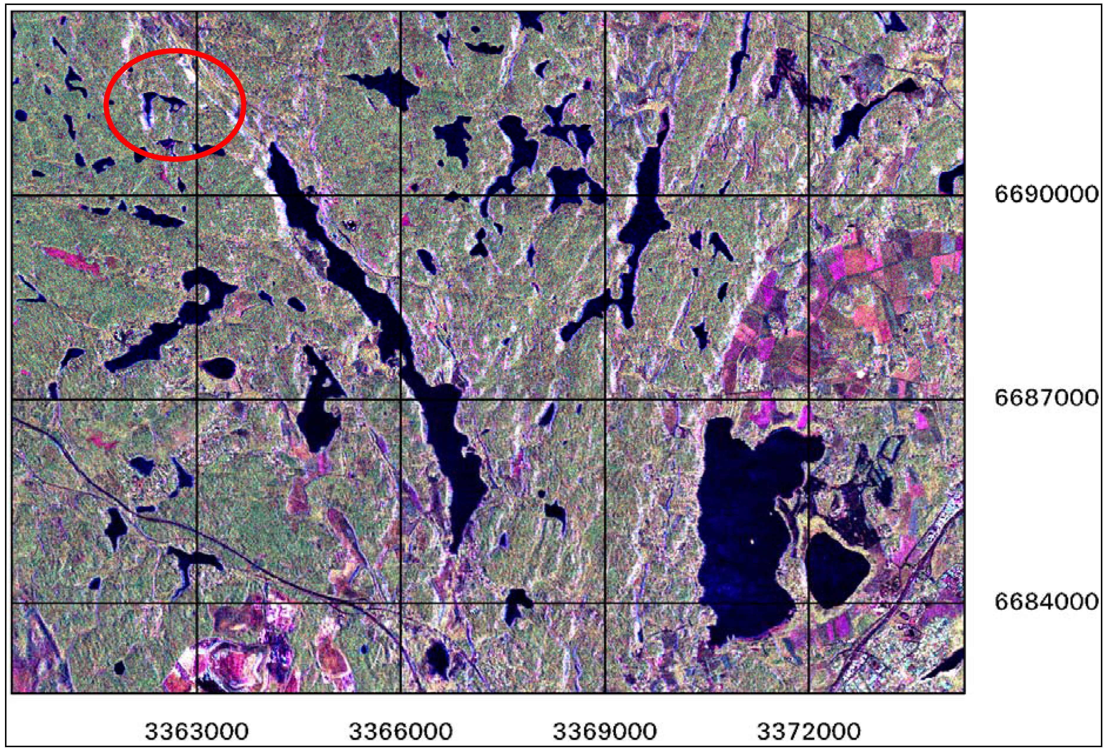
Processing of the TerraSAR-X images was carried out at the Finnish Geodetic Institute (FGI). First, all images were converted to intensity images (squared amplitude), because in this study only the amplitude information of the backscattering was used (interferometric processing can be applied only to images with same imaging geometries). In order to extract plot-level specific forest information, the images should be accurately registered with each other and with existing topographic maps. Because the side-looking imaging geometry of SAR causes image distortions, a Digital Elevation Model (DEM) and a proper geocoding model was used in the orthorectification process. In this study, the PCI Geomatica software (PCI Geomatics, Richmond Hill, Ontario, Canada) and the DEM of the National Land Survey of Finland with a ground sampling distance of 25 m were used. The resulting RMS errors using 26 ground control points were 4.5 meters in the easting direction and 3.8 meters in the northing direction. The ground control points were acquired from the digital maps of the National Land Survey of Finland. Finally, the orthorectified images were visually compared to the digital maps and a very good agreement was observed. Therefore, we can safely assume that the geometric accuracy should be good enough to extract plot level information. A false color fusion of all seven images is presented in
Figure 1. In this case, black and dark blue areas correspond to water bodies whereas bright white areas correspond to build-up environment, but also to areas of steep slopes, which are facing to the satellite. Green areas are covered by forest. The field plots are located in the north-west corner in
Figure 1.
Figure 1.
False color fusion of all used TerraSAR-X images (Red: average amplitude of co-polarized image channels, Green: average amplitude of cross-polarized image channels, and Blue: standard deviation of amplitude of all image channels). Map projection: Finnish Uniform Coordinate System. Original Data © 2008–2009, German Aerospace Center.
To collect SAR features, circles with radii of 20 m were formed using the centre points of the field plots. The SAR feature extraction unit was larger than the field plot (radius 7.98 m). However, the field plot stand characteristics were assumed to represent stand characteristics in the SAR feature extraction unit. The use of the 20-m radii ensured that enough TerraSAR-X pixels could be used to calculate the average backscattering intensity and its standard deviation for the test plots. After calculation of the average intensity, radiometric normalization was applied to the intensity values. In the radiometric normalization, the method based on the projection angle was used [
22]. The projection angle based method uses the local slope and aspect angles of the surface calculated from a DEM. Then, the TerraSAR-X features were converted back to the amplitude scale (square root of intensity). Therefore, the used set consisted of 28 TerraSAR-X features (average amplitude and standard deviation for seven images with two polarization channels) for each plot. Very high backscattering values can be expected for steep barren cliffs facing to the satellite. Therefore, all field plots having slope angles higher than 15°, which typically correspond to the barren cliffs, were excluded from the further studies. Finally, the TerraSAR-X features of the test plots were exported to feature selection and the plot-level forest variable estimation.
2.4. Genetic Algorithm and Feature Selection
Generally, adding more features in the estimation process improves the output accuracy, but with increasing dimensionality the distinctive capacity of the data may weaken, with increasing noise. Therefore, the dimensionality of large datasets must be reduced. The usefulness of any input variable can be studied by measuring the correlation between the image features and forest attributes, but this method does not reveal the combined behaviour of the features. Thus, filters that rank features based on correlation coefficients are not sufficient and subset selection algorithms or feature transformation is needed. In our earlier studies we have found genetic algorithms (GAs) suitable for this task [
23]. GAs are search algorithms that mimic natural selection and natural genetics [
24].
In model construction, it is important to base the feature selection on the researcher's knowledge of the phenomenon and the variables affecting it; thus the use of stepwise selection methods is generally discouraged. However, there are situations in which the superiority of variables A and B over C and D is not clear. The relationships of recorded radiation or returned laser pulses and forest variables are not too straightforward (the exception being the canopy surface generated from laser height readings) and there are numerous potentially useful statistical/textural variables that can be extracted from the data. Therefore, the use of automated selection methods is justified to a certain extent.
The following feature sets were created:
A: 28 TerraSAR-X features
B: 48 laser features
A + B (76 different features)
Features selected from set A using GA
Features selected from set B using GA
Features selected from set A+B using GA
Feature sets A, B and A+B were used for benchmarking the results obtained with feature selection by GA. Automatic feature selection was carried out using a simple GA presented by Goldberg [
24], implemented in the GAlib C++ library [
25]. The GA process starts by generating an initial population of strings (chromosomes or genomes) that consist of separate features (genes). The strings evolve during a user-defined number of iterations (generations). The evolution includes the following operations: selecting strings for mating, using a user-defined objective criterion, letting the strings in the mating pool swap parts (crossing over), causing random noise (mutations) in the offspring (children) and passing the resulting strings into the next generation.
In the present study, the starting population consisted of 300 random feature combinations (genomes). The length of the genomes corresponded to the total number of features in each step, and the genomes contained a 0 or 1 at position i, denoting the absence or presence of image feature i. The number of generations was 30. The objective variable was a weighted combination of relative RMSEs of Vol, Hg, Dg, VolP, VolS and VolD, with total volume having a weight of 50% and the rest 10% each. Genomes selected for mating swapped parts with each other with a probability of 80%, producing children. Occasional mutations (flipping 0 to 1 or vice versa) were added to the children (probability 1%). The strings were then passed to the next generation. The overall best genome of the current iteration was always passed to the next generation, as well.
Three consecutive steps were taken to reduce the number of features to a reasonable minimum. Since the algorithm starts from a random pool of genomes, the process was repeated three times at each step. Only features belonging to the best genome of the three repetitions in each step were included in the next step.
2.5. Estimation of Plot-Level Forest Variables
The
k-NN method was used in the forest variable estimation (e.g., [
26,
27], (Equation 1)). A central assumption is that field plots (or stands) that are similar in reality will be similar in the space defined by remotely sensed data features, as well. The forest variables of any image pixel can then be estimated with the help of reference field plots measured in the field by calculating the averages of the
k nearest neighbours. In the present study, similarity was determined by the Euclidean distances in the image feature space. Before calculation of Euclidean distances all features were standardized to a mean of 0 and std of 1. The nearest neighbours were weighted with inverse distances (Equation 2):
where:
ŷ = estimated value for variable y
yi = measured value for variable y at the i:th nearest field plot
w = weight of field plot i in the estimation
k = number of neighbours used in the estimation
An essential parameter affecting the results obtained with the k-NN method is the number of neighbours, k, for which a value of 5 was set in this study. Selecting the value for k is always a compromise: a small k increases the random error of the estimates, while a large k results in averaged estimates and reduces the variation available in the original dataset.
2.6. Evaluation of Estimation Accuracy
Evaluation of the estimation accuracy was carried out using leave-one-out cross-validation. In the process, each field plot at a time is left out of the reference dataset and the forest variable estimates are calculated using the remaining field plots. The estimates are then compared with the values observed in the field. The RMSE (Equation 3), BIAS (Equation 5), relative RMSE (Equation 4) and relative BIAS (Equation 6) were derived from the comparisons:
where:
n = number of plots
yi = observed value for plot i
= predicted value for plot i
= observed mean of the variable in question.
3. Results
The relative RMSEs and biases obtained, using the features selected with GA (reduced feature sets) are presented in
Table 3 and those obtained with the original, large feature sets in
Table 4. The results show that the ALS-based features performed far better than the TerraSAR-X -based features. The combined feature set improved the Vol, BA and Hg results slightly. Generally, Hg and Dg were estimated more accurately than Vol and BA. Both remote sensing materials resulted in somewhat biased results.
Table 3.
Relative RMSEs and relative biases (in parentheses), % of means, of the estimated stand characteristics using the reduced feature sets.
Table 3.
Relative RMSEs and relative biases (in parentheses), % of means, of the estimated stand characteristics using the reduced feature sets.
| | ALS | TerraSAR-X | Combined |
|---|
| Vol | 35.7 (−2.0) | 55.8 (0.6) | 34.7 (−1.5) |
| BA | 28.7 (−2.1) | 43.8 (0.0) | 28.1 (−1.4) |
| Hg | 14.7 (−0.1) | 20.8 (0.3) | 14.3 (−0.3) |
| Dg | 21.2 (−0.2) | 26.6 (−0.9) | 21.4 (0.2) |
| VolP | 98.5 (2.2) | 133.7 (2.8) | 99.9 (10.0) |
| VolS | 60.1 (−1.5) | 128.9 (−0.2) | 61.6 (−4.4) |
| VolD | 83.2 (−7.2) | 138.2 (−0.6) | 91.6 (−9.5) |
| Features used | 12 | 7 | 12 |
Table 4.
Relative RMSEs and relative biases (in parentheses), % of means, of the estimated stand characteristics using the original feature sets.
Table 4.
Relative RMSEs and relative biases (in parentheses), % of means, of the estimated stand characteristics using the original feature sets.
| | ALS | TerraSAR-X | Combined |
|---|
| Vol | 39.5 (−1.9) | 65.5 (3.2) | 39.2 (−1.9) |
| BA | 31.1 (−2.7) | 49.7 (2.1) | 31.7 (−2.4) |
| Hg | 14.4(1.0) | 21.5 (0.4) | 15.4 (−0.0) |
| Dg | 20.4 (1.3) | 26.2 (0.0) | 21.5 (0.5) |
| VolP | 106.9 (7.9) | 139.2 (9.6) | 119.8 (8.7) |
| VolS | 70.2 (1.6) | 142.0 (−2.3) | 78.3 (−0.7) |
| VolD | 95.7 (−17.8) | 151.6 (4.9) | 99.8 (−15.4) |
| Features used | 48 | 28 | 76 |
Reduced feature sets outperformed the original sets: the Vol RMSE percentages decreased by 4–8 percentage points during the GA selection process. The biases were mainly reduced as well. The number of features selected by GA for the final sets were 12, 7 and 12 for the ALS, TerraSAR-X and combined set, respectively. When both ALS and TerraSAR-X features were available, both types were included in the final set as well. However, the majority of the features selected were based on ALS height statistics (9 of 12).
Tree species-specific mean volumes were estimated with significantly larger errors than the combined mean volumes. Most accurate results were obtained for the tree species dominating in volume, Norway spruce, except in the case of the original TerraSAR-X feature set.
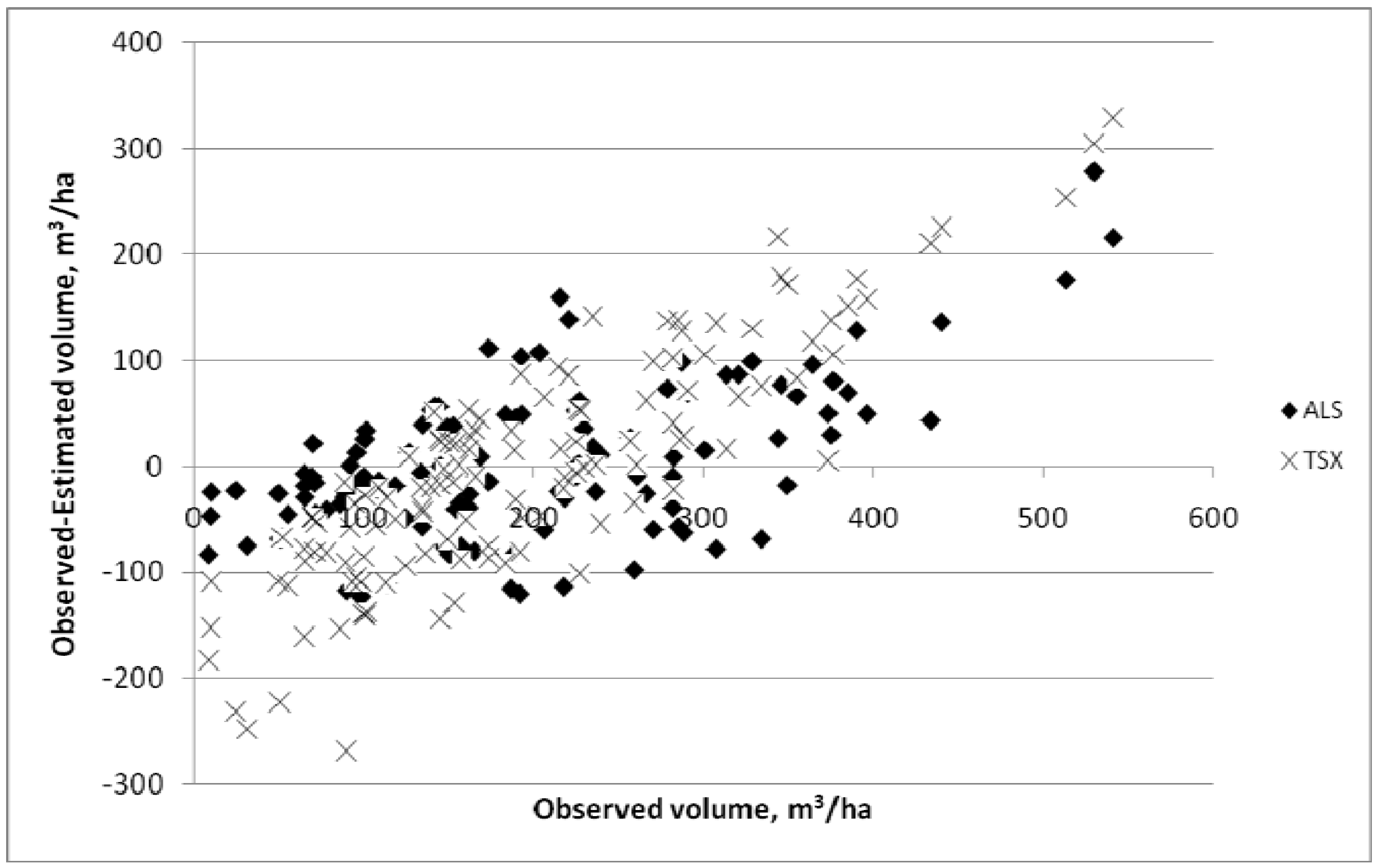
Plot-by-plot comparison of Vol estimation errors by means of TerraSAR-X features and ALS-based features is shown in
Figure 1. It can be seen that TerraSAR-X systematically overestimates the smallest volumes and underestimates the largest volumes. Laser-based features performed better at both ends of the volume range.
Figure 2.
Volume estimation errors (VolObs-VolEst) with best performing ALS and TerraSAR-X feature sets.
Figure 2.
Volume estimation errors (VolObs-VolEst) with best performing ALS and TerraSAR-X feature sets.
4. Conclusions
In the present study, important forest attributes were estimated for forest management planning using a combination of low-pulse ALS and TerraSAR-X data, GA feature selection and the nonparametric k-NN algorithm. The lowest RMSEs were obtained with relatively small subsets of the original features. Results obtained with large, original feature sets had higher RMSEs and biases than the final subsets. Improvements via the feature selection process were the greatest in the case of the TerraSAR-X feature set.
The RMSE obtained for stem volume was 34.7%. TerraSAR-X features, when used separately from ALS features, gave significantly higher errors, confirming that the ALS data were superior to the TerraSAR-X data. However, some TerraSAR-X features were selected into the combined feature set. ALS and TerraSAR-X RMSEs tended to be lower than with Landsat-type satellite images, which usually result in field plot-level RMSEs of 60% or greater [
14,
23,
28]. The ALS accuracies were in line with other Finnish studies operating with low-pulse density data (e.g., [
17,
20]), but with slightly poorer results. This was probably a result from the small number of study plots in
k-NN estimation and greater variation in the stand characteristics of the study area, compared with earlier studies.
As noticed in earlier studies (e.g., [
19,
29]) the tree species dominating in the area, Norway spruce, was estimated with the highest accuracy among the tree species. The relative RMSEs were largest for Scots pine, which had a mean volume similar to deciduous tree species, but much lower maximum volumes.
The mean errors of traditional ocular forest inventory used in operational forest management planning vary from 16% to 38% in Finland [
30,
31,
32]. This means that the approximately 30% error level reached with the combined dataset at the field plot level resembles that of ocular field inventory (the ALS and TerraSAR-X RMSEs are probably somewhat lower at the stand level).
It should be pointed out that because of small number of study plots, our findings can be seen as preliminary. It was not possible to split our study to training and testing datasets and we had to use leave-one-out cross-validation procedure.
A central task for future forest resource inventories will be detection of changes, i.e., updating the forest inventory data. In addition to the traditional forest variables, more interest will be placed on changes in biomass, bioenergy and carbon balance. Climate change will probably increase forest damage, creating a demand for monitoring methods as well.
When comparing our TerraSAR-X accuracy to the E-SAR accuracies achieved by Holopainen
et al. [
14], plot-level volume and BA estimations were poorer with TerraSAR-X. However, the Hg and Dg estimations were slightly better. Our results suggest that currently available non-interferometric SAR features cannot compete with ALS in large-scale precision forestry. The combined feature set only slightly outperformed ALS feature set in the case of general stand variables, but was poorer in the case of species-specific volumes. This is similar result to the results achieved by Nelson
et al. [
12], who concluded that ALS is a better choice over SAR in forest biomass estimation and SAR only slightly increased the overall accuracy when ALS and SAR were used jointly in the estimation.
The exploitation of SAR images is still challenging at the moment due to the high costs, somewhat troublesome processing and tricky imaging geometries. However, we believe that high-resolution satellite SAR images may play a significant future role in nationwide forest mapping applications, due to the higher temporal repeatability in comparison to ALS data acquisition. One promising alternative may be the use of SAR images for updating forest inventories performed with help of low-pulse ALS data. A very promising technique in forestry seems to be Single-pass SAR interferometry in X band (TerraSAR-X/TanDEM-X), which may provide useful information of the stand height. Moreover, the combination of polarimetric and interferometric information is expected to increase the accuracy of forest parameter estimation when compared to use of backscattering intensity only.


 ,
, 