DEM Development from Ground-Based LiDAR Data: A Method to Remove Non-Surface Objects


Abstract
:1. Introduction
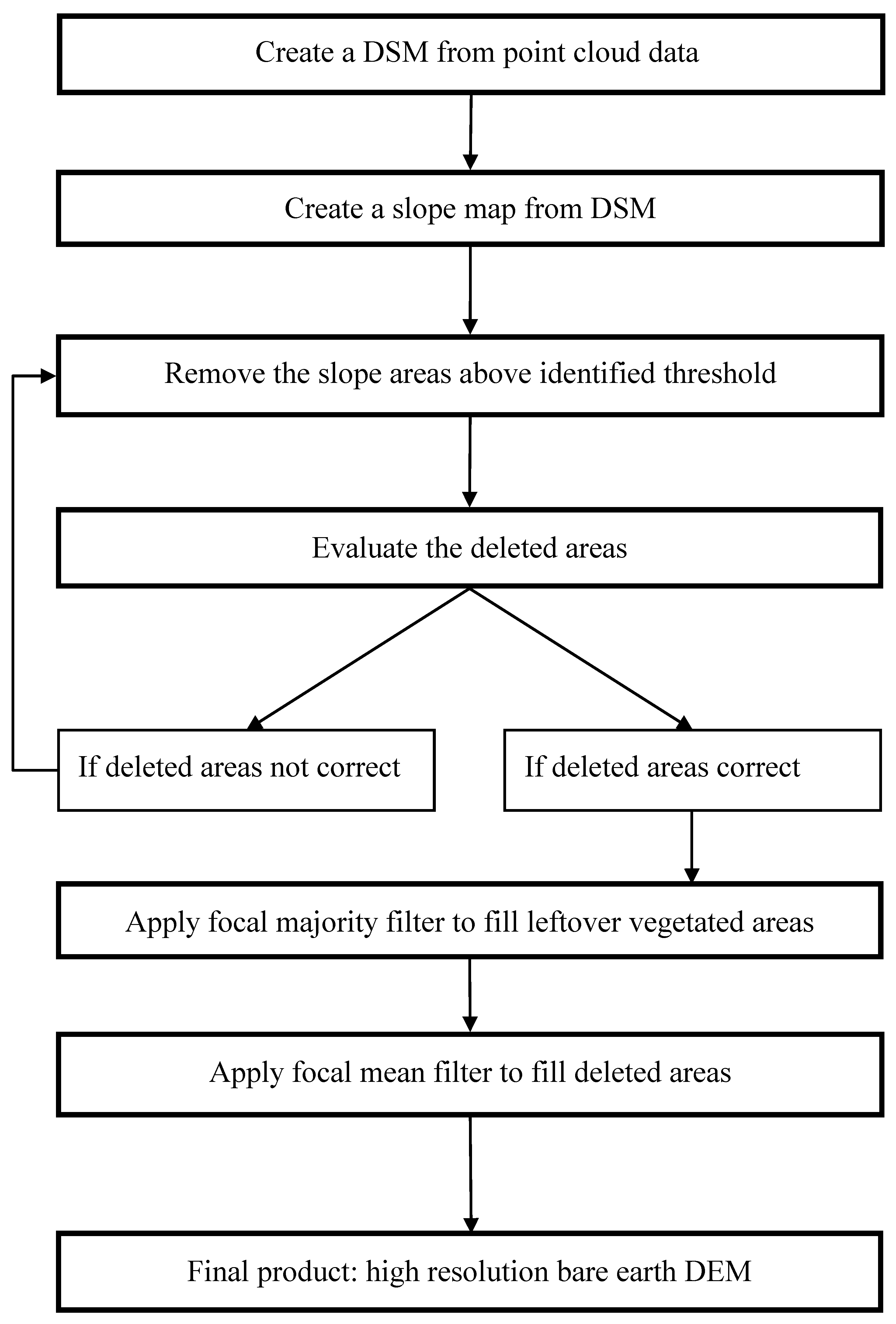
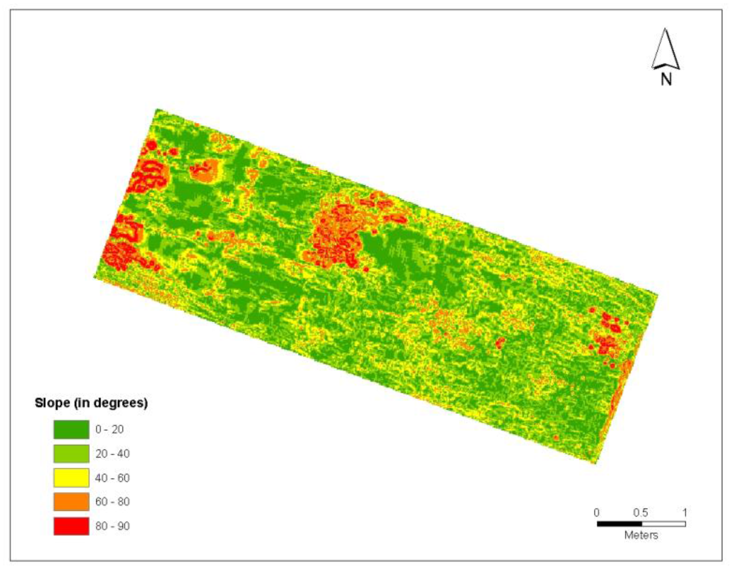
2. Methods
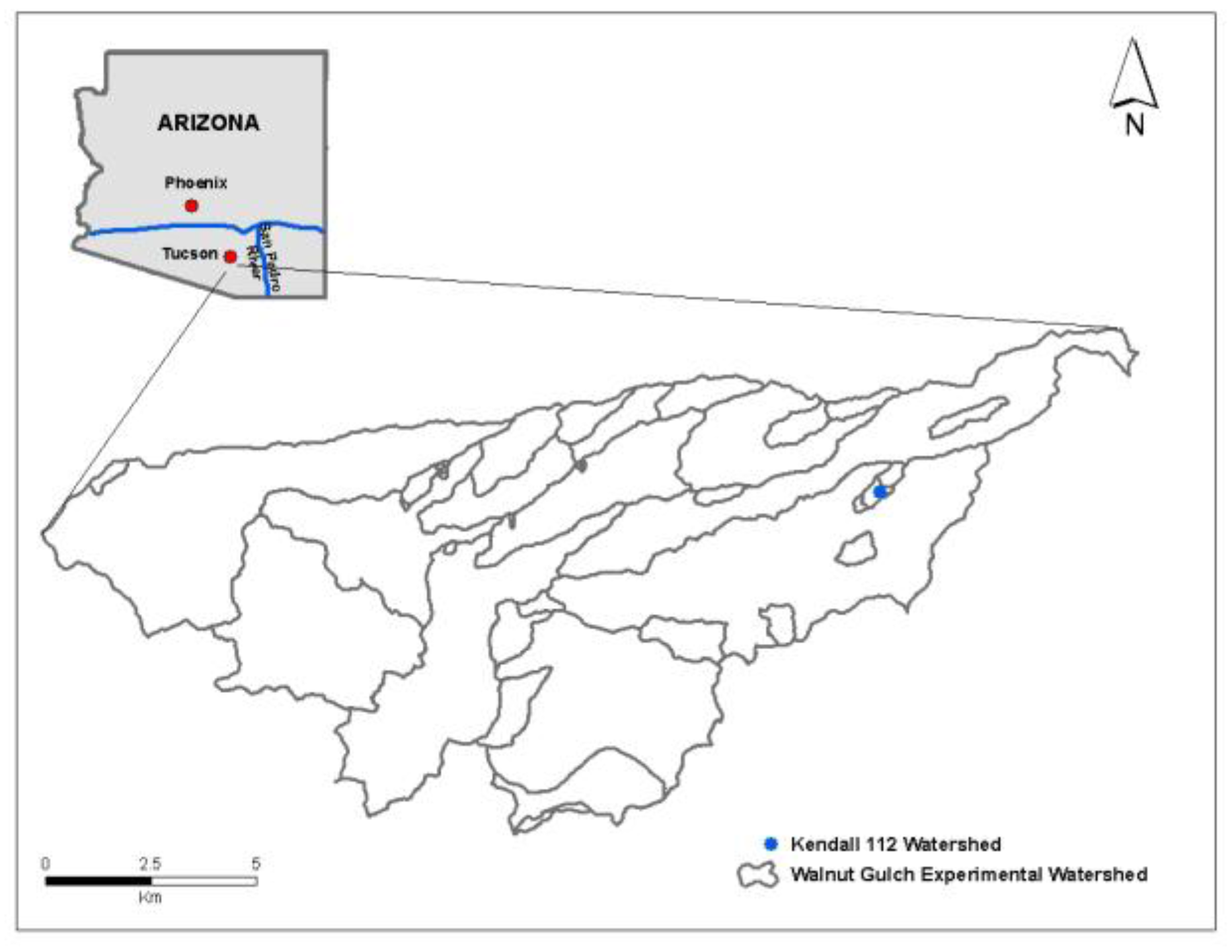
2.1. Study Area
2.2. Ground-Based LiDAR Unit and Data Acquisition
2.3. Validation

3. Results and Discussion
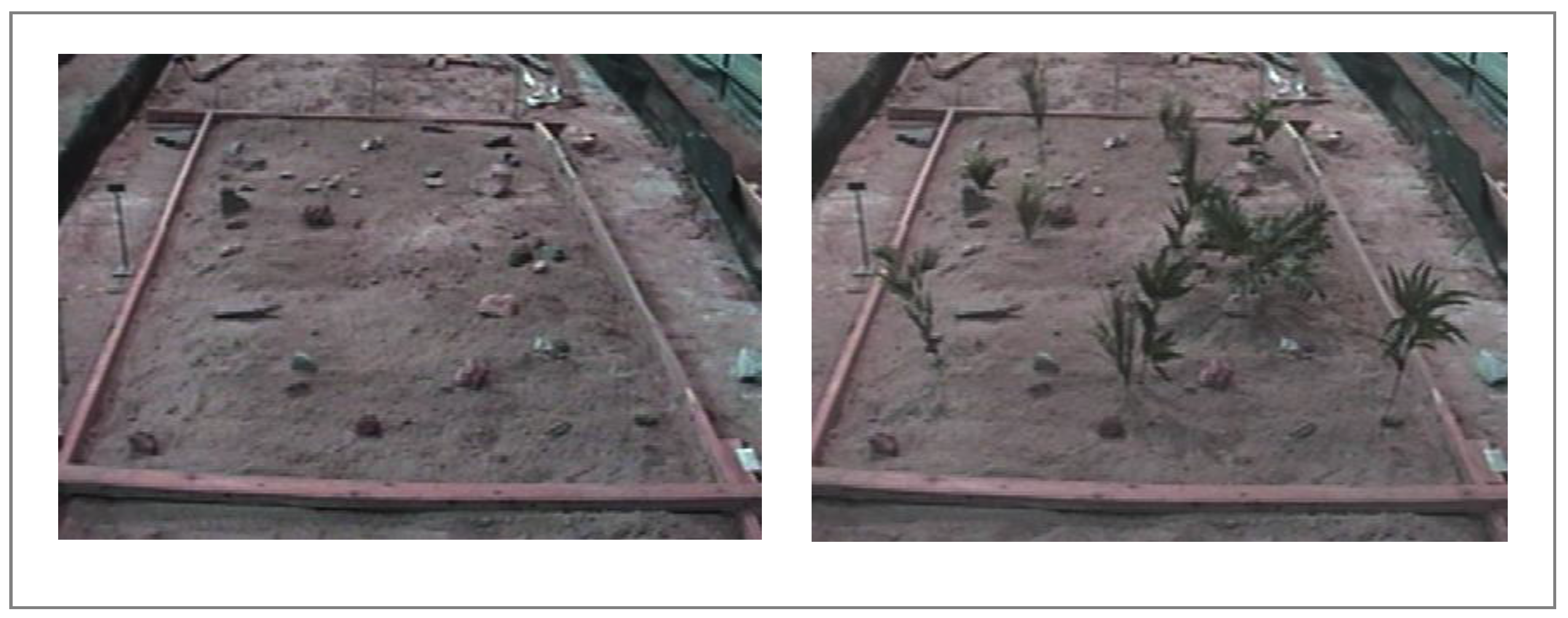
3.1. Field Plots


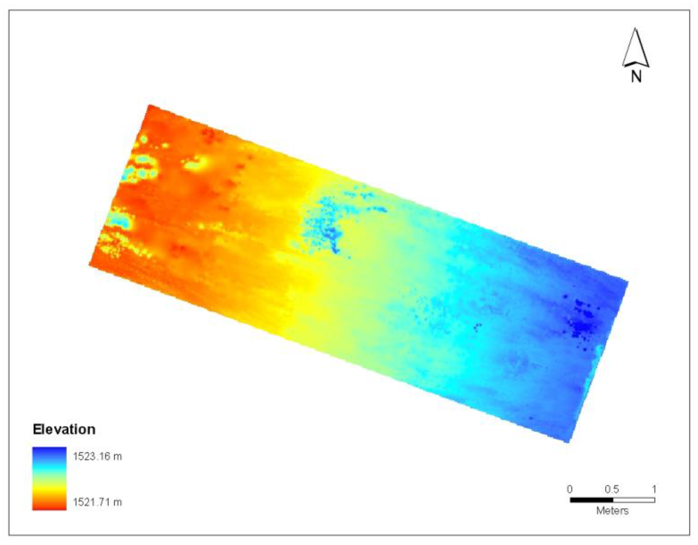
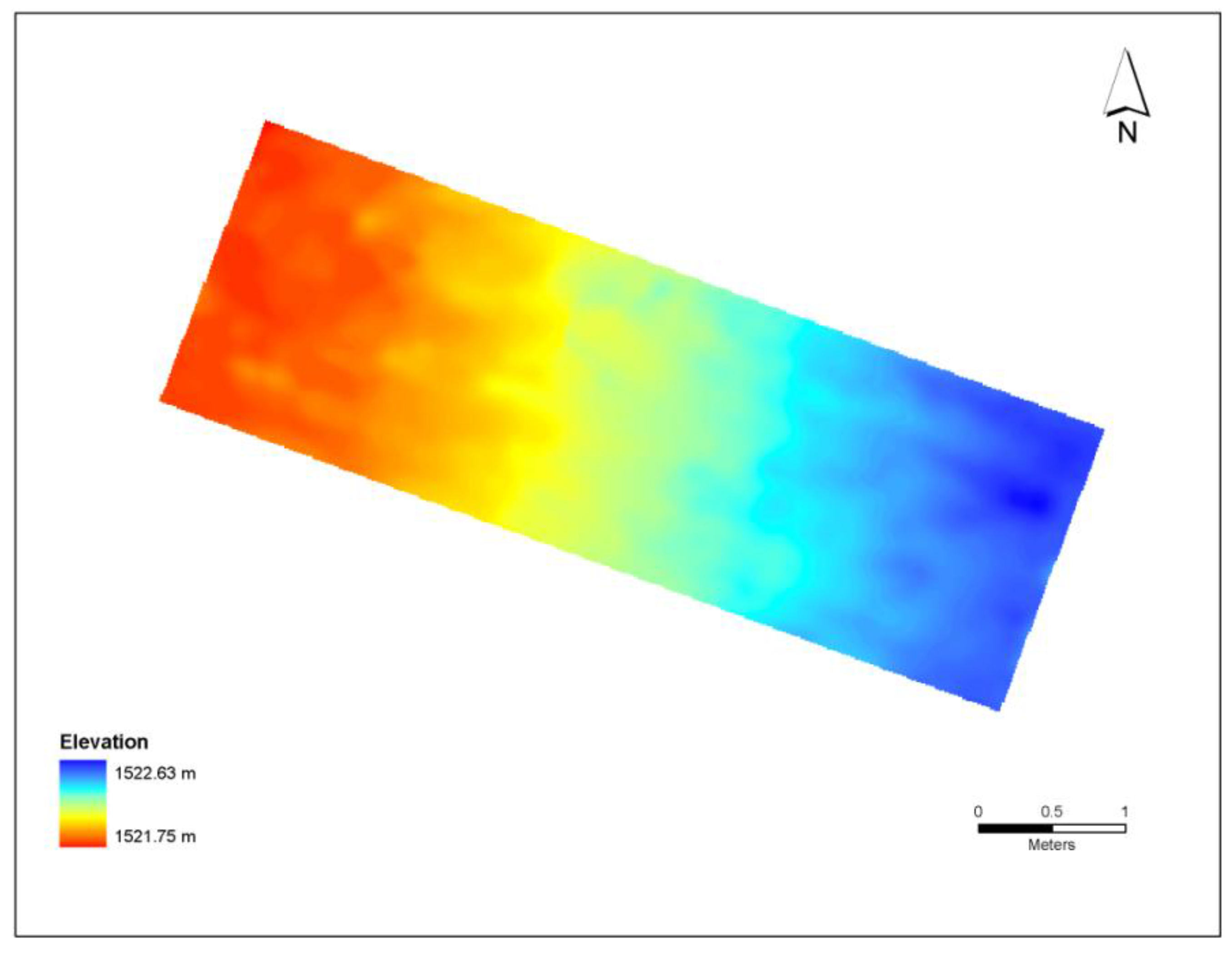
| DSM | DEM | |
|---|---|---|
| Minimum (m) | 1521.71 | 1521.75 |
| Maximum (m) | 1523.17 | 1522.63 |
| Mean (m) | 1522.18 | 1522.16 |
| Standard Deviation | 0.25 | 0.25 |
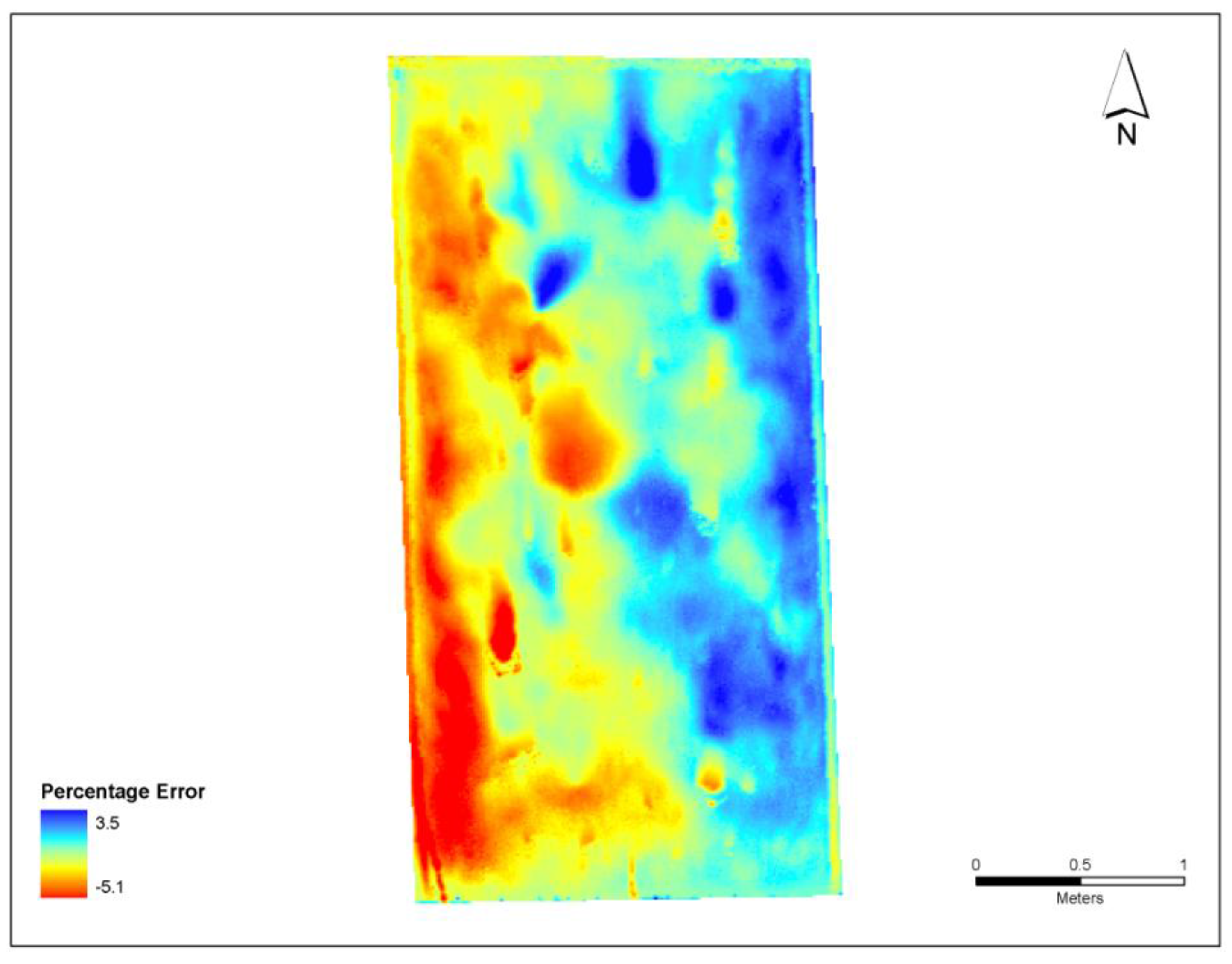
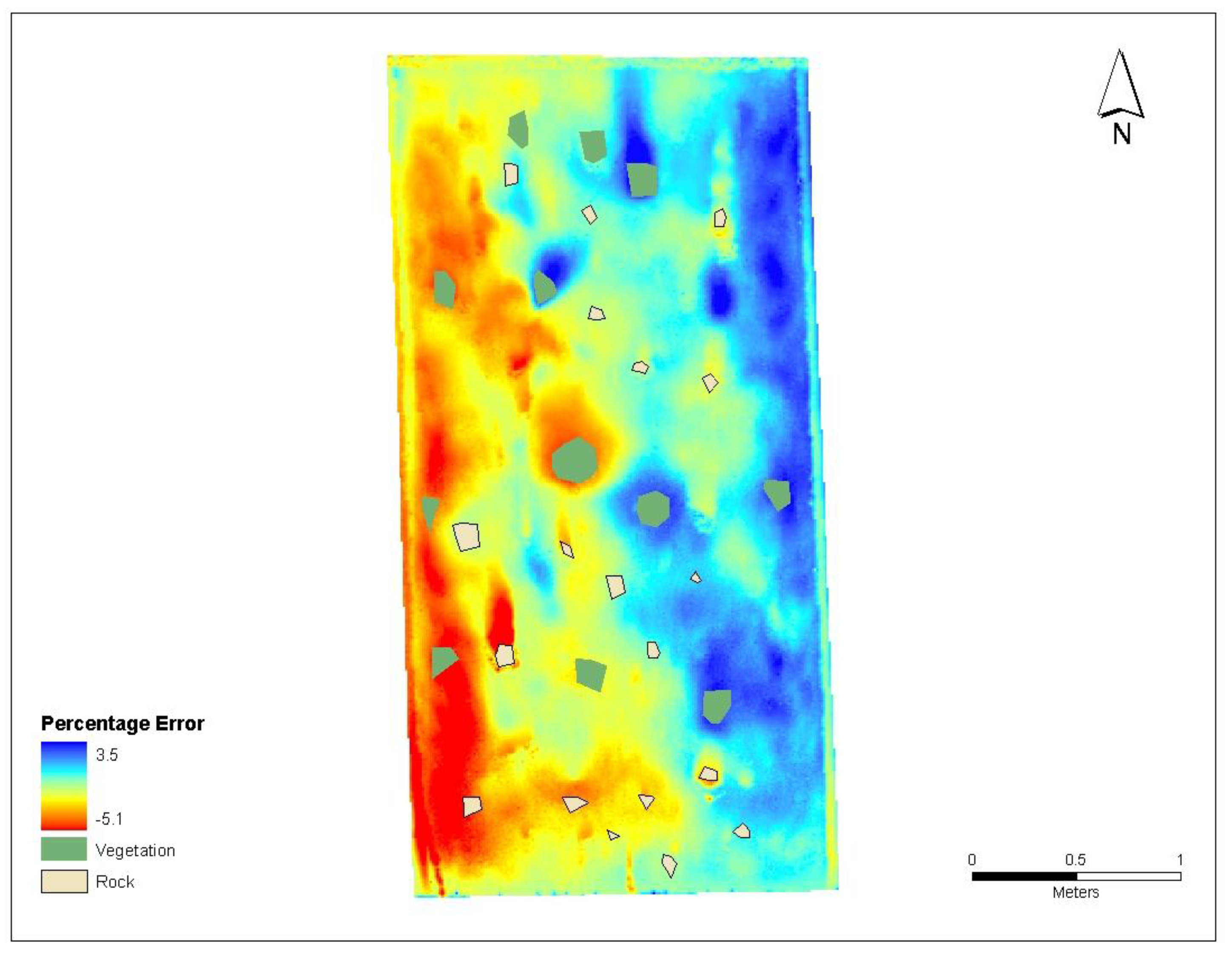
3.2. Validation Plot Results


3.3. Implications
| DSM | final DEM | |
|---|---|---|
| Minimum (m) | 3.87 | 3.92 |
| Maximum (m) | 4.78 | 4.80 |
| Mean (m) | 4.34 | 4.36 |
| Standard Deviation | 0.22 | 0.23 |
4. Conclusions
Acknowledgements
References
- Miller, S.N.; Semmens, D.J.; Goodrich, D.C.; Hernandez, M.; Miller, R.C.; Kepner, W.G.; Guertin, D.P. The automated geospatial watershed assessment tool. Environ. Model. Softw. 2007, 22, 365–377. [Google Scholar] [CrossRef]
- Bowen, H.Z.; Waltermire, R.G. Evaluation of light detection and ranging (LiDAR) for measuring river corridor topography. J. Amer. Water Resour. Assoc. 2002, 38, 33–41. [Google Scholar] [CrossRef]
- Bobba, A.G.; Bukata, R.P.; Jerome, J.H. Digitally processed satellite data as a tool in detecting potential groundwater flow systems. J. Hydrol. 1992, 131, 25–62. [Google Scholar] [CrossRef]
- Haugerud, R.A.; Harding, D.J. Some algorithms for Virtual Deforestation (VDF) of LIDAR topographic survey data. Int. Arch. Photogramm. Remote Sens. 2001, 34, 211–217. [Google Scholar]
- Axelsson, P. DEM generation from laser scanner data using adaptive TIN models. Int. Arch. Photogramm. Remote Sens. 2000, 33, 110–117. [Google Scholar]
- Elmqvist, M. Ground surface estimation from airborne laser scanner data using active shape models. Int. Arch. Photogramm. Remote Sens. 2002, 34, 114–118. [Google Scholar]
- Brovelli, M.; Cannata, M.; Longoni, U. Lidar data filtering and DTM interpolation within Grass. Trans. GIS 2004, 8, 155–174. [Google Scholar] [CrossRef]
- Wick, J.W. Interface-Total Station in Archaeology. Soc. Amer. Archaeol. Bull. 1 1996, 14, 16. [Google Scholar]
- Frohlich, C.; Mittenleiter, M. Terrestrial laser scanning—New perspective in 3D surveying. Int. Arch. Photogramm. Remote Sens. 2004, 36, 1–7. [Google Scholar]
- Opitz, D.; Blundell, S. Hierarchical Feature Extraction: Removing the Clutter. In Proceedings of International ESRI User Conference, San Diego, CA, USA, 2002; pp. 51–52.
- Kilian, J.; Haala, N.; Englich, M. Capture and evaluation of airborne laser scanner data. Int. Arch. Photogramm. Remote Sens. 1996, 31, 383–388. [Google Scholar]
- Vossleman, G. Slope based filtering of laser altimetry data. Int. Arch. Photogramm. Remote Sens. 2000, 33, 935–942. [Google Scholar]
- Roggero, M. Airborne laser scanning: Clustering in raw data. Int. Arch. Photogramm. Remote Sens. 2001, 34, 227–232. [Google Scholar]
- Pfeifer, N.; Kostli, A.; Kraus, K. Interpolation and filtering of laser scanner data—Implementation and first results. Int. Arch. Photogramm. Remote Sens. 1998, 32, 153–159. [Google Scholar]
- Hodgson, M.E.; Jensen, J.; Raber, G.; Tullis, J.; Davis, B.A.; Thompson, G.; Schuckman, K. An evaluation of lidar-derived elevation and terrain slope in leaf-off conditions. Photogramm. Eng. Remote Sensing 2005, 71, 817–823. [Google Scholar] [CrossRef]
- Lim, K.; Wulder, M.; St-Onge, B.; Flood, M. LiDAR remote sensing of forest structure. Prog. Phys. Geogr. 2007. [Google Scholar] [CrossRef]
- Renard, K.J.; Lane, L.J.; Simanton, J.R.; Emmerich, W.E.; Stone, J.J.; Weltz, M.A.; Goodrich, D.C.; Yakowitz, D.S. Agricultural impacts in an Arid Environment: Walnut Gulch Studies. In Proceedings of 2nd US/CIS joint conf. on Environmental Hydrology and Hydrogeology, Arlington, VA, USA, May 1993; pp. 16–20.
- Paige, G.B.; Stone, J.J.; Guertin, P.; Lane, L.J. A strip model approach to parameterize a coupled Green-Ampt kinematic wave model. J. Amer. Water Resour. Assoc. 2002, 38, 1363–1377. [Google Scholar]
- Optech, ILRIS-3D, Intellegent Laser Ranging and Imaging System 2004. Available online: http://www.ilris-3d.com (accessed on 15 October 2007).
- Polyworks Software Version 9.0, 2007. Available online: www.innovmetric.com (accessed on 26 June 2006).
- Burrough, P.A.; McDonnell, R.A. Principles of Geographical Information Systems; Oxford University Press: Oxford, UK, 2004; p. 333. [Google Scholar]
- ESRI, ArcGIS 9.0. 26 June 2007. Available online: http://www.esri.com (accessed on 26 June 2007).
- Tomlin, D.C. Geographic Information Systems and Cartographic Modeling; Prentice Hall College Division: Englewood Cliffs, NJ, USA, 1990; p. 572. [Google Scholar]
© 2010 by the authors; licensee MDPI, Basel, Switzerland. This article is an open access article distributed under the terms and conditions of the Creative Commons Attribution license (http://creativecommons.org/licenses/by/3.0/).
Share and Cite
Sharma, M.; Paige, G.B.; Miller, S.N. DEM Development from Ground-Based LiDAR Data: A Method to Remove Non-Surface Objects. Remote Sens. 2010, 2, 2629-2642. https://doi.org/10.3390/rs2112629
Sharma M, Paige GB, Miller SN. DEM Development from Ground-Based LiDAR Data: A Method to Remove Non-Surface Objects. Remote Sensing. 2010; 2(11):2629-2642. https://doi.org/10.3390/rs2112629
Chicago/Turabian StyleSharma, Maneesh, Ginger B. Paige, and Scott N. Miller. 2010. "DEM Development from Ground-Based LiDAR Data: A Method to Remove Non-Surface Objects" Remote Sensing 2, no. 11: 2629-2642. https://doi.org/10.3390/rs2112629
APA StyleSharma, M., Paige, G. B., & Miller, S. N. (2010). DEM Development from Ground-Based LiDAR Data: A Method to Remove Non-Surface Objects. Remote Sensing, 2(11), 2629-2642. https://doi.org/10.3390/rs2112629