Modeling and Correction of Underwater Photon-Counting LiDAR Returns Based on a Modified Biexponential Distribution

Highlights

What are the main findings?

• A Modified Biexponential Distribution (MBD) model is proposed to accurately characterize the asymmetric shape of underwater single-photon LiDAR return pulses, effectively representing both sharp rising and long-tailed decay behaviors.
• The proposed model-driven IRF matching framework mitigates underwater pulse broadening effects and improves ranging accuracy without the need for labor-intensive underwater calibration.

What are the implications of the main findings?

• The MBD model significantly enhances depth estimation accuracy in turbid underwater environments, achieving a 17.54 percentage reduction in Depth Absolute Error and a 50 percentage increase in the probability of precise ranging.
• This work establishes a robust analytical foundation for improving photon detection and bathymetric performance in underwater LiDAR systems, supporting future applications in marine mapping and underwater exploration.

Abstract

Laser pulses experience significant temporal broadening in underwater environments due to strong turbulence and scattering effects. As water turbidity increases, the likelihood of multiple scattering events rises, further intensifying pulse broadening and thereby degrading the ranging accuracy of underwater single-photon LiDAR systems. Accurate characterization of the return pulse shape is crucial for precise distance extraction, typically achieved via cross-correlation with the system’s Instrument Response Function (IRF). Conventional models often fail to accurately characterize the distinctive asymmetric shape of underwater LiDAR returns, which feature a rapid rise and a slow decay. To address this limitation, this paper proposes a Modified Biexponential Distribution (MBD) model, specifically designed to capture both the sharp leading edge and the gradual trailing decay of the pulses. This model enables a more accurate representation of the broadened pulse, effectively mitigating the ranging error induced by scattering. Experimental validation demonstrates that, at an attenuation length of 6.9, the Depth Absolute Error (DAE) is reduced from 3.82 cm to 3.15 cm (a 17.54% improvement), while the probability of achieving a DAE below 3.82 cm increases from 49.70% to 74.83%. These results confirm the effectiveness and robustness of the proposed model in enhancing the ranging accuracy of underwater photon-counting LiDAR systems. Furthermore, this study provides a model-driven analytical basis for improving underwater photon detection and bathymetric performance in turbid conditions.

1. Introduction

Underwater optics technology has emerged as a powerful tool for applications such as marine resource exploration, underwater archaeology, and bathymetric mapping [1,2,3]. Single-photon detection technology, with its ultra-high sensitivity at the photon level and picosecond-scale temporal resolution, plays a pivotal role in advancing next-generation underwater LiDAR systems [4,5]. Recent developments in single-photon LiDAR have enabled high-resolution underwater imaging and bathymetry under strong scattering conditions [6,7,8]. Building on these foundations, current research is extending the technology in two key directions: toward more compact system designs [9], and toward advanced downstream processing—such as adaptive 3D reconstruction from noisy photon sequences [10], depth-profile-based target discrimination [11], and end-to-end object recognition via multi-modal data fusion [12]. However, the performance of all these high-level tasks fundamentally relies on the accuracy and reliability of the raw ranging measurements for each pixel or data point. Underwater environments are inherently affected by strong scattering, severe attenuation, and random turbulence [13,14], which cause significant energy loss and temporal broadening of laser pulses. In this study, random turbulence refers to stochastic fluid disturbances that enhance optical scattering. These effects jointly degrade the accuracy and stability of underwater ranging measurements [15].

Conventional distance estimation techniques are typically based on peak-detection and cross-correlation algorithms. The peak-detection approach directly estimates distance from the maximum of the LiDAR return signal but is highly susceptible to underwater backscatter and Poisson noise [16]. In contrast, cross-correlation with the Instrument Response Function (IRF) provides higher accuracy; however, deviations between theoretical and measured IRFs—mainly caused by pulse broadening during propagation—introduce significant errors [17,18,19]. Consequently, accurate modeling and compensation of pulse broadening are critical for reliable underwater ranging.

Several models have been proposed to characterize LiDAR reflected signals, including the Gaussian distribution model [20], the Improved Gaussian Distribution (IGD) model [21], and multi-segment piecewise functions [22]. The Gaussian model is widely adopted due to its simplicity and low parameter count but fails to capture the inherent asymmetry of underwater returns. The IGD model partially improves the fit in the trailing region of the peak but cannot represent the rapid rising edge, limiting its robustness under noise. Multi-segment models enhance fitting accuracy but suffer from excessive complexity and computational cost, hindering real-time applicability.

To overcome these limitations, this paper introduces a pulse broadening correction method based on a Modified Biexponential Distribution (MBD). The proposed model integrates the advantages of both the biexponential and Gaussian functions, enabling accurate representation of the sharp rising edge and gradual decay of underwater return signals. This approach effectively mitigates pulse broadening while providing a model-driven IRF matching framework that reduces reliance on cumbersome underwater calibration. Building upon this framework, distance extraction via cross-correlation achieves significantly improved ranging accuracy. To validate the method, we performed laboratory experiments on underwater targets. The results demonstrate that, compared with conventional models, the MBD approach yields superior fitting accuracy and ranging performance, thereby offering a reliable solution for high-precision underwater single-photon LiDAR systems.

The main contributions of this work are threefold:

Modified Return—We propose an MBD model that accurately characterizes the asymmetric features of underwater return signals, effectively capturing both the steep rising edge and the long-tailed decay behavior inherent in single-photon LiDAR echoes.

IRF Matching Framework—We establish a model-driven Instrument Response Function (IRF) matching framework that mitigates pulse broadening effects without the need for labor-intensive underwater calibration procedures, thereby enhancing the robustness and practicality of underwater LiDAR systems.

Experimental Validation—We validate the proposed approach through controlled laboratory experiments, demonstrating that the MBD model achieves superior fitting accuracy and significantly improves ranging performance compared with conventional Gaussian, IGD, and piecewise models.

Collectively, these contributions provide a reliable theoretical and technical foundation for advancing high-precision ranging and imaging in underwater single-photon LiDAR systems.

2. Methods

2.1. Traditional LiDAR Return Model

2.1.1. Gaussian-Distributed Return Signal Model

The Gaussian distribution is widely used to model LiDAR return signals due to its mathematical simplicity. The emitted laser pulse itself generally exhibits a Gaussian-like energy distribution, and Gaussian modeling facilitates signal processing and feature extraction. As such, the Gaussian distribution has been extensively employed to approximate LiDAR return signals, as expressed in Equation (1):

$$f(t,p_G)={\displaystyle \frac{N_G}{\sqrt{2\pi }{\sigma }_G}}exp\left[-{\displaystyle \frac{{(t-t_l)}^2}{2{\sigma }_G^2}}\right]$$

(1)

where $p_G=(N_G,{\sigma }_G,t_l)$ denotes the parameter set of this model. Specifically, $N_G$ is the amplitude correction coefficient, ${\sigma }_G$ is the reflected pulse width (taken as the full width at half maximum, FWHM), and $t_l$ is the peak position of the Gaussian function.

The Gaussian distribution offers a concise model with few parameters, which are readily derivable from the LiDAR system’s physical characteristics. However, it struggles to accurately capture the asymmetric features of underwater return waveforms. The inherent symmetry of the Gaussian function makes it unsuitable for modeling complex underwater environments.

2.1.2. Improved Gaussian-Distributed Return Signal Model

Ove Steinvall first proposed an improved Gaussian distribution (IGD) for LiDAR return modeling [21]. The key modification introduces a time-dependent damping factor into the Gaussian formulation to simulate the gradual decay of the falling edge of the laser pulse, thereby improving the representation of asymmetric return signals. The model is expressed as Equation (2):

$$f(t,p_I)=\beta {\left({\displaystyle \frac{t-t_l}{\tau }}\right)}^{2}exp\left[-{\displaystyle \frac{t-t_l}{\tau }}\right]$$

(2)

where $p_I=(\beta ,\tau ,t_l)$ is the parameter set, with $\beta$ as the amplitude correction factor, $\tau$ as the pulse width (often taken as the FWHM of the emitted pulse), and $t_l$ is the peak position of the IGD.

The IGD maintains low computational complexity and effectively simulates the slow decay behavior of post-peak returns [22], outperforming the standard Gaussian model in this respect. However, it fails to capture the rapid rise before the peak, resulting in reduced fitting accuracy and weak noise robustness. Consequently, it is inadequate for signal reconstruction in highly scattering underwater conditions.

2.1.3. Piecewise Function Models

To improve simple distribution models, piecewise functions have been introduced to approximate complex LiDAR return signals. For instance, Gerald’s group at Heriot-Watt University proposed a four-segment exponential model for photon-counting returns [22,23], expressed as:

$$f(t,p_p)=\beta ·\left\{\begin{array}{cc}exp\left[{\displaystyle \frac{t-t_1}{t_1}}-{\displaystyle \frac{{(t_1-t_l)}^2}{2{\sigma }^2}}\right],\hfill & t<t_1\hfill \\ exp\left[-{\displaystyle \frac{{(t-t_l)}^2}{2{\sigma }^2}}\right],\hfill & t_1\le t<t_2\hfill \\ exp\left[-{\displaystyle \frac{t-t_1}{t_2}}-{\displaystyle \frac{{(t_2-t_l)}^2}{2{\sigma }^2}}\right],\hfill & t_2\le t<t_3\hfill \\ exp\left[-{\displaystyle \frac{t_3-t_2}{t_2}}-{\displaystyle \frac{t-t_3}{t_3}}-{\displaystyle \frac{{(t_2-t_l)}^2}{2{\sigma }^2}}\right],\hfill & t_3\le t\hfill \end{array}\right.$$

(3)

where $f(t,p_p)=(\beta ,\sigma ,t_l,t_1,{\tau }_1,t_2,{\tau }_2,t_3,{\tau }_3)$ denotes the parameter set of this model. $\beta$ represents the return signal amplitude correction factor; $\sigma$ is the width factor of the piecewise Gaussian function, characterizing the smoothness of the piecewise function (indeed denotes the standard deviation); $t_l$ denotes the peak timing of the segmented function; $(t_1,t_2,t_3)$ denotes the segmented times of the piecewise function; $({\tau }_1,{\tau }_2,{\tau }_3)$ represents the characteristic parameters of the exponential distribution within the piecewise function. The four distinct segments of the distribution are: the model’s rising segment, the model’s peak segment, and the model’s falling segment, expressed by two segmented functions. This approach improved fitting accuracy at the cost of even greater complexity. The exponential growth of parameters significantly reduces the model’s universality and real-time applicability.

2.2. Modified Biexponential Distribution Model

The MBD is designed to capture the asymmetric characteristics of underwater photon-counting returns while maintaining manageable complexity.

The time response of carriers generated in the depletion layer of SPAD detectors typically follows a Gaussian distribution. However, early-arriving photons in the neutral region induce carrier diffusion, producing exponential-like distortions in the response distribution [24,25]. To accurately capture this composite behavior, we adopt a convolution of Gaussian and biexponential distributions [26]. This yields a model that retains Gaussian-like characteristics in the central region while preserving the heavy-tailed behavior of the biexponential distribution.

The Gaussian and biexponential models are defined as:

$$g(t,\sigma ,t_l)={\displaystyle \frac{1}{\sqrt{2\pi }\sigma }}exp\left(-{\displaystyle \frac{{(t-t_l)}^2}{2{\sigma }^2}}\right)$$

(4)

$$f(t,t_l,b_1,b_2)=\left\{\begin{array}{cc}{\displaystyle \frac{1}{2b_1}}exp\left(-{\displaystyle \frac{t_l-t}{b_1}}\right),\hfill & t<t_l\hfill \\ {\displaystyle \frac{1}{2b_2}}exp\left(-{\displaystyle \frac{t-t_l}{b_2}}\right),\hfill & t\ge t_l\hfill \end{array}\right.$$

(5)

$f_B(t,p_B)$ is the probability density function (PDF) of the modified double exponential distribution, as shown in Equation (6), where ⊗ denotes the convolution operation:

$$\begin{array}{cc}\hfill f_B(t,p_B)& =f(t,t_l,\sigma )\otimes g(t,t_l,b_1,b_2)={\int }_{-\infty }^{+\infty }f\left(x\right)g(t-x)dx\hfill \\ \hfill & ={\int }_{-\infty }^{t_l}f\left(x\right)g(t-x)dx+{\int }_{t_l}^{+\infty }f\left(x\right)g(t-x)dx\hfill \\ \hfill & ={\displaystyle \frac{1}{2\sqrt{2\pi }\sigma b_1}}exp\left({\displaystyle \frac{-\frac{2{\sigma }^2{t}_l+b_1{(t-t_l)}^2}{b_1}+{\left(\frac{{\sigma }^2+b_1(t-t_l)}{b_1}\right)}^2}{2{\sigma }^2{b}_1}}\right)\hfill \\ \hfill & \times {\int }_{-t_l}^{+\infty }exp\left(-{\displaystyle \frac{{\left(v+\frac{{\sigma }^2+b_1(t-t_l)}{b_1}\right)}^2}{2{\sigma }^2{b}_1}}\right)dv\hfill \\ \hfill & +{\displaystyle \frac{1}{2\sqrt{2\pi }\sigma b_2}}exp\left({\displaystyle \frac{-\frac{b_2{(t_l-t)}^2-2{\sigma }^2{t}_l}{b_2}+{\left(\frac{{\sigma }^2+b_2(t_l-t)}{b_2}\right)}^2}{2{\sigma }^2{b}_2}}\right)\hfill \\ \hfill & \times {\int }_{t_l}^{+\infty }exp\left(-{\displaystyle \frac{{\left(x+\frac{{\sigma }^2+b_2(t_l-t)}{b_2}\right)}^2}{2{\sigma }^2{b}_2}}\right)dx\hfill \end{array}$$

(6)

Therefore, the final expression for the probability density function MBD of the modified double exponential distribution is shown as Equation (7):

$$\begin{array}{cc}\hfill f_B(t,p_B)& =f(t,t_l,\sigma )\otimes g(t,t_l,b_1,b_2)={\int }_{-\infty }^{+\infty }f\left(x\right)g(t-x)dx\hfill \\ \hfill & ={\displaystyle \frac{1}{4b_1}}exp\left({\displaystyle \frac{{\sigma }^2}{2b_1^2}}+{\displaystyle \frac{t-2t_l}{b_1}}\right)\mathrm{erfc}\left({\displaystyle \frac{-t_l+\frac{{\sigma }^2+b_1(t-t_l)}{b_1}}{\sqrt{2}\sigma }}\right)\hfill \\ \hfill & +{\displaystyle \frac{1}{4b_2}}exp\left({\displaystyle \frac{{\sigma }^2}{2b_2^2}}+{\displaystyle \frac{2t_l-t}{b_2}}\right)\mathrm{erfc}\left({\displaystyle \frac{t_l+\frac{{\sigma }^2+b_2(t_l-t)}{b_2}}{\sqrt{2}\sigma }}\right)\hfill \end{array}$$

(7)

where $\mathrm{erfc}(·)$ is the complementary error function. The parameter set is $p_B=(\sigma ,b_1,b_2,t_l)$, where $\sigma$ defines the return pulse width, $t_l$ is the peak position, and $b_1$, $b_2$ control the rising and falling slopes, respectively.

$$\mathrm{erfc}\left(x\right)={\displaystyle \frac{2}{\sqrt{\pi }}}{\int }_x^{\infty }{e}^{-y^2}dy$$

(8)

Compared with Gaussian and IGD models, the MBD introduces only modest parameter complexity while achieving superior fitting accuracy. Relative to multi-segment functions, the MBD drastically reduces the parameter count, avoids basis function selection issues, and significantly lowers computational cost, making it well-suited for practical underwater LiDAR applications.

2.3. Methods Implementation

Figure 1 illustrates the overall workflow of the proposed underwater single-photon ranging method. The approach integrates signal acquisition and preprocessing with IRF-based system calibration and effective target echo extraction. Based on these steps, pulse shape modeling is performed to enable accurate depth retrieval using the proposed MBD.

Key parameters, including the peak position of the underwater target echo and the pulse width of the calibrated IRF (e.g., full width at half maximum), are extracted to constrain the pulse modeling process. A conventional Gaussian distribution is first employed as a baseline to assess the limitations of symmetric pulse assumptions in underwater environments. To more faithfully describe the asymmetric rising and decaying behavior of broadened underwater return pulses, a biexponential distribution model is subsequently introduced. Building upon these models, the proposed MBD integrates their respective advantages, providing a more accurate representation of underwater return pulses and thereby improving ranging precision.

3. Experimental System

3.1. Experimental Setup and Environment

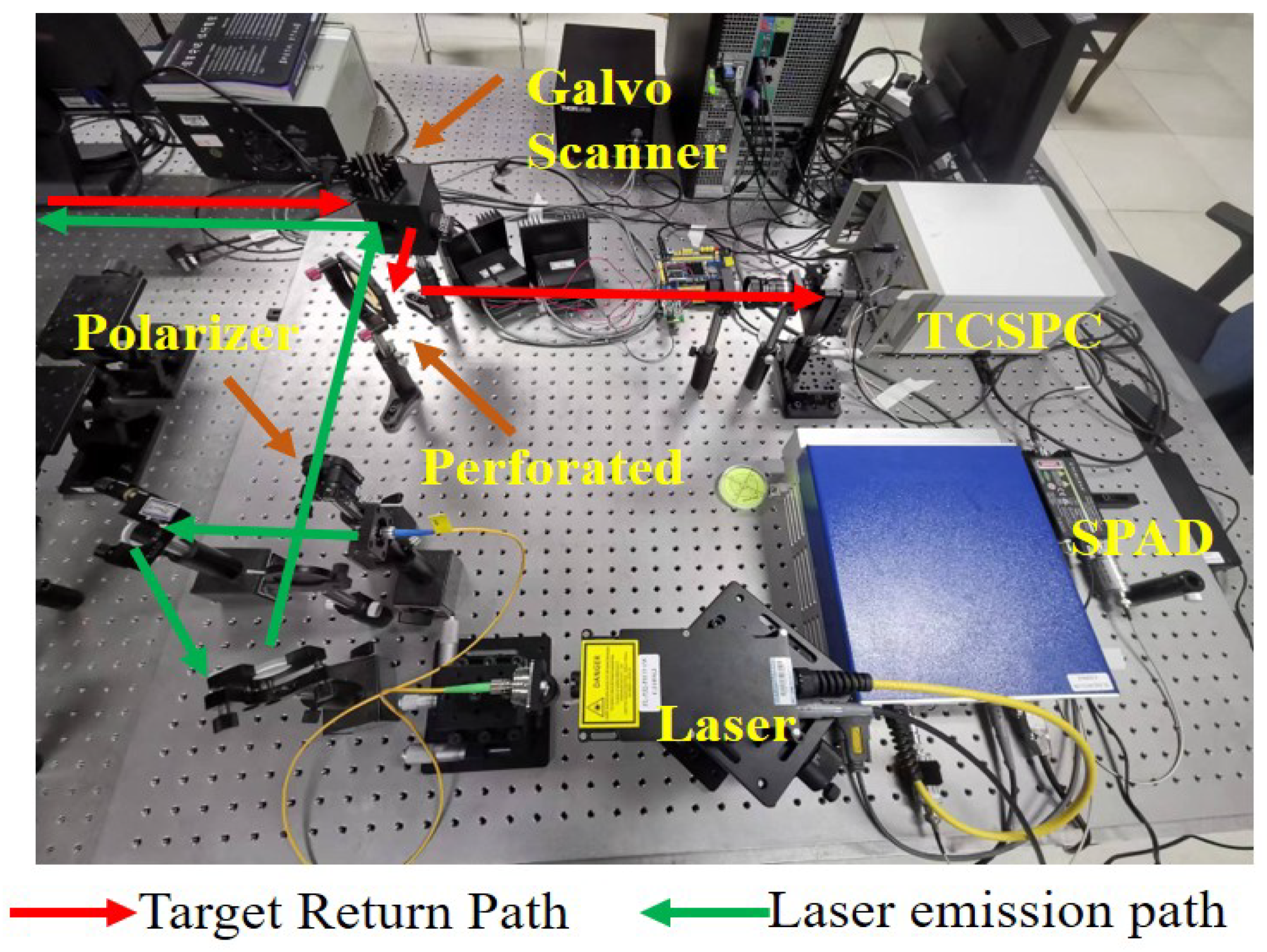
A 532 nm laser serves as the light source, with the pulsed laser selected as the FL-532-PICO-1W pulsed fiber laser from Changchun New Industrial Optoelectronics Technology Co., Ltd. (Changchun, Jilin, China). The single-photon avalanche diode (SPAD) detector utilizes the SPCM-AQRH-16-FC detector from Excelitas (Waltham, MA, USA). The TCSPC counter employs the PicoHarp 300 time-correlated single-photon counting module from PicoQuant (Berlin, Germany). The control unit is a computer based on an Intel(R) Core(TM) i7-9700 CPU.

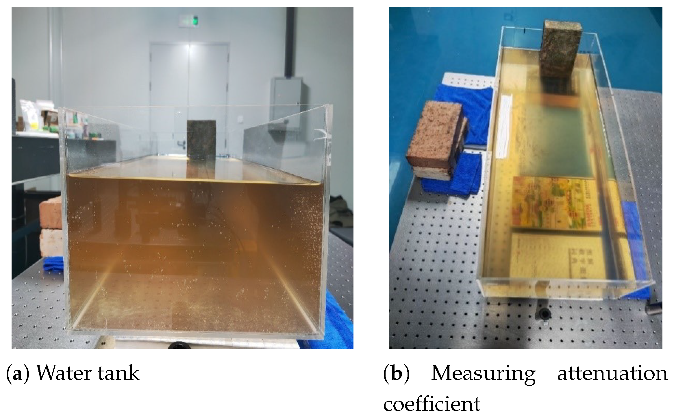
The experimental setup is shown in Figure 2. The experimental scenario is depicted in Figure 3, where the target (brick) is placed in a water tank measuring 80 cm in length, positioned 74.5 cm from the front edge of the tank wall. The reference true distance of the underwater target is established as 74.5 cm. This value was calculated by measuring the target’s thickness in air using a vernier caliper, then subtracting this measurement from the total internal length (80.0 cm) of the standardized rectangular tank.

3.2. Attenuation Coefficient Calibration Experiment

The attenuation coefficient calibration schematic is shown in Figure 4.

According to the Lambert–Beer law, the attenuation coefficient is given by Equation (9).

$$\alpha ={\displaystyle \frac{-ln(P_b/(P_f\times 0.72))}{d}}$$

(9)

where $P_b$ denotes the laser power after exiting the water tank, $P_f$ denotes the laser power before entering the water tank, and d represents the length of the water tank, i.e., the distance the laser travels through the water.

Figure 4. Experimental setup for attenuation coefficient calibration.

Figure 4. Experimental setup for attenuation coefficient calibration.

The experiments were conducted in a darkroom environment. Background noise, as measured using an OPHIR PD300-3W-v1 optical power meter (MKS Instruments, Jerusalem, Israel), was maintained below 5 nW. A long accumulation time of 120 s was used to minimize uncertainties arising from statistical fluctuations. To simulate a highly scattering and attenuating underwater environment, SiO₂ powder and mulberry juice were introduced into clear water. The laser power measured prior to the window of the water tank was 2.85 mW, while the power detected after transmission through the water was 1.3 uW. The single-pass transmittance of the empty tank was 85.65%, corresponding to an attenuation coefficient of 9.23 m⁻¹. With the target placed at an underwater depth of 74.5 cm, the attenuation length was determined to be 6.9. Detailed experimental parameters are summarized in

Table 1. Main parameters of the system.

Parameter	Value
Wavelength	532 nm
Laser pulse width	501 ps@532 nm
Average output power of the laser	2.85 mW
Pulse repetition frequency	1 MHz
Single-point cumulative time	120 s
Photon detection efficiency	50%
Dead time	22 ns
Bin width	4 ps

.

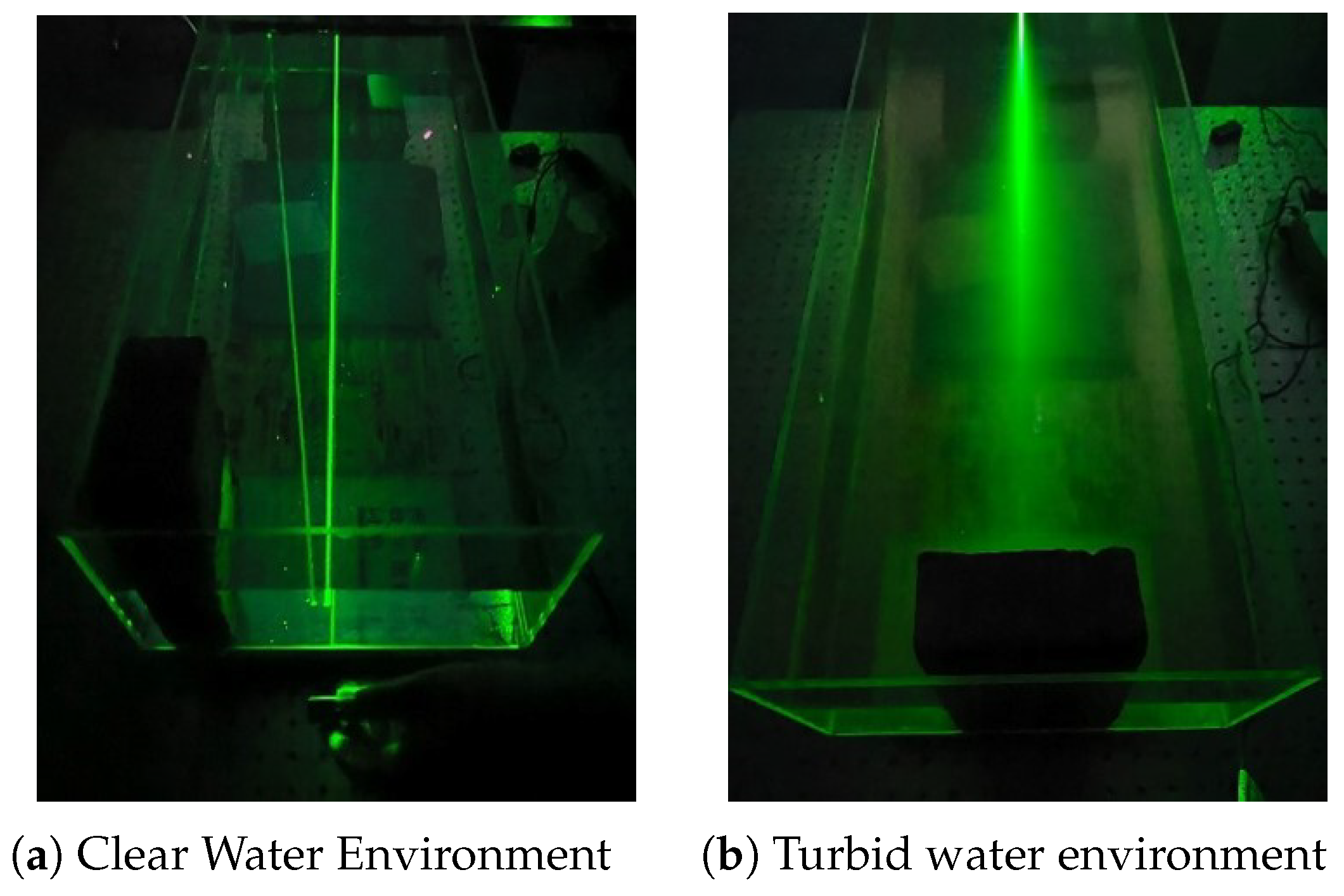
To more clearly demonstrate the extent of scattering effects on laser transmission underwater, Figure 5 presents a comparison of laser propagation in clear versus turbid water within a darkroom environment.

4. Results and Discussion

4.1. Experimental Analysis

The experiment involved constructing an underwater single-photon imaging system and simulating real aquatic environments using mixed solutions. The obtained experimental data were analyzed and validated. The existing model’s fitting accuracy was verified using the experimental data, while simultaneously investigating the phenomenon of laser pulse broadening as it propagates through complex aquatic media.

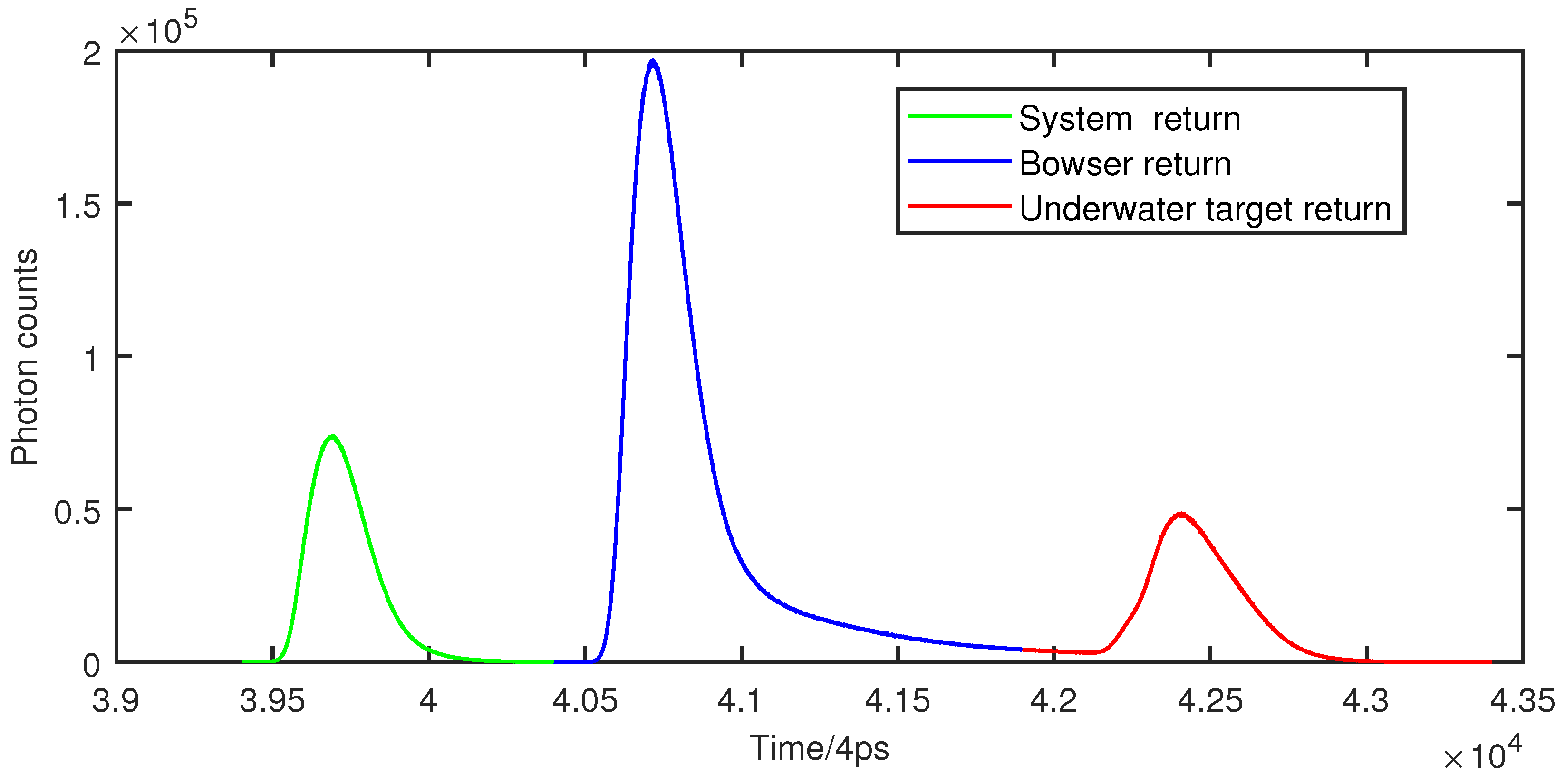
As shown in Figure 5, pronounced laser scattering occurs during underwater light propagation. The time-correlated single-photon counting (TCSPC) system was operated in T2 mode to acquire raw data over 250,000 time bins with a temporal resolution of 4 ps. For subsequent analysis, the relevant signal segment corresponding to the target peak region (bins 39,401 to 43,200) was extracted.

Figure 6 displays this extracted signal segment, where three distinct echo peaks are visible. The first green waveform corresponds to the system echo from the two-dimensional scanning mirror, the second blue waveform represents the echo from the window of the water tank, and the third red waveform corresponds to the underwater target return. The first two can be regarded as air-based echoes. The FWHM values of the system echo and wall echo are 218 ps and 225 ps, respectively, while that of the underwater target echo increases to 302 ps, clearly indicating pulse broadening that degrades ranging accuracy. The detailed parameters of the three echoes are summarized in

Table 2. Numerical information corresponding to Figure 5.

	System Return	Bowser Return	Underwater Target Return
Peak position	293	1317	3007
FWHM	218	225	302

.

To avoid potential signal distortions caused by the glass wall interface—which could introduce systematic offsets in distance measurement—the internal optical system return is adopted here as an ideal photon-counting echo signal. Based on this reference signal, Gaussian, IGD, Piecewise, and the proposed MBD method are applied for fitting. All signals are uniformly normalized for comparison.

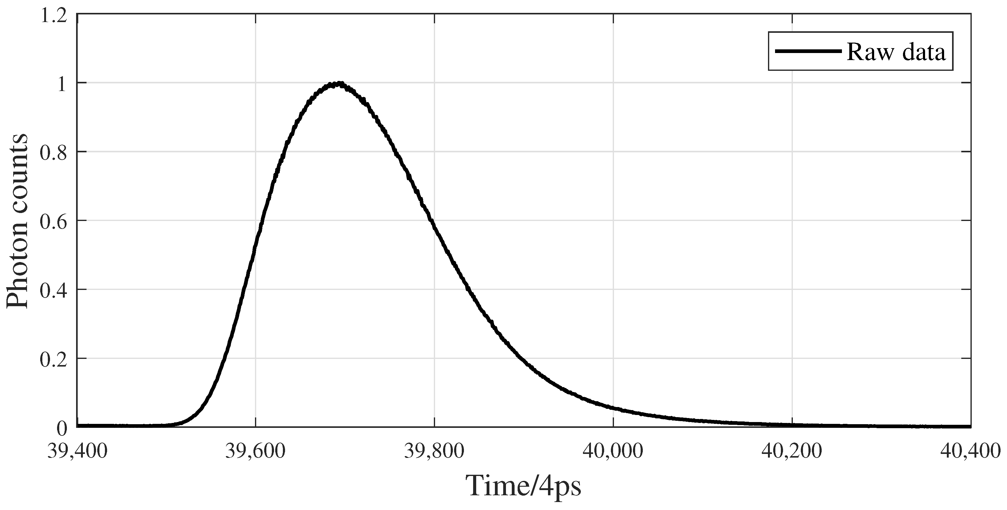
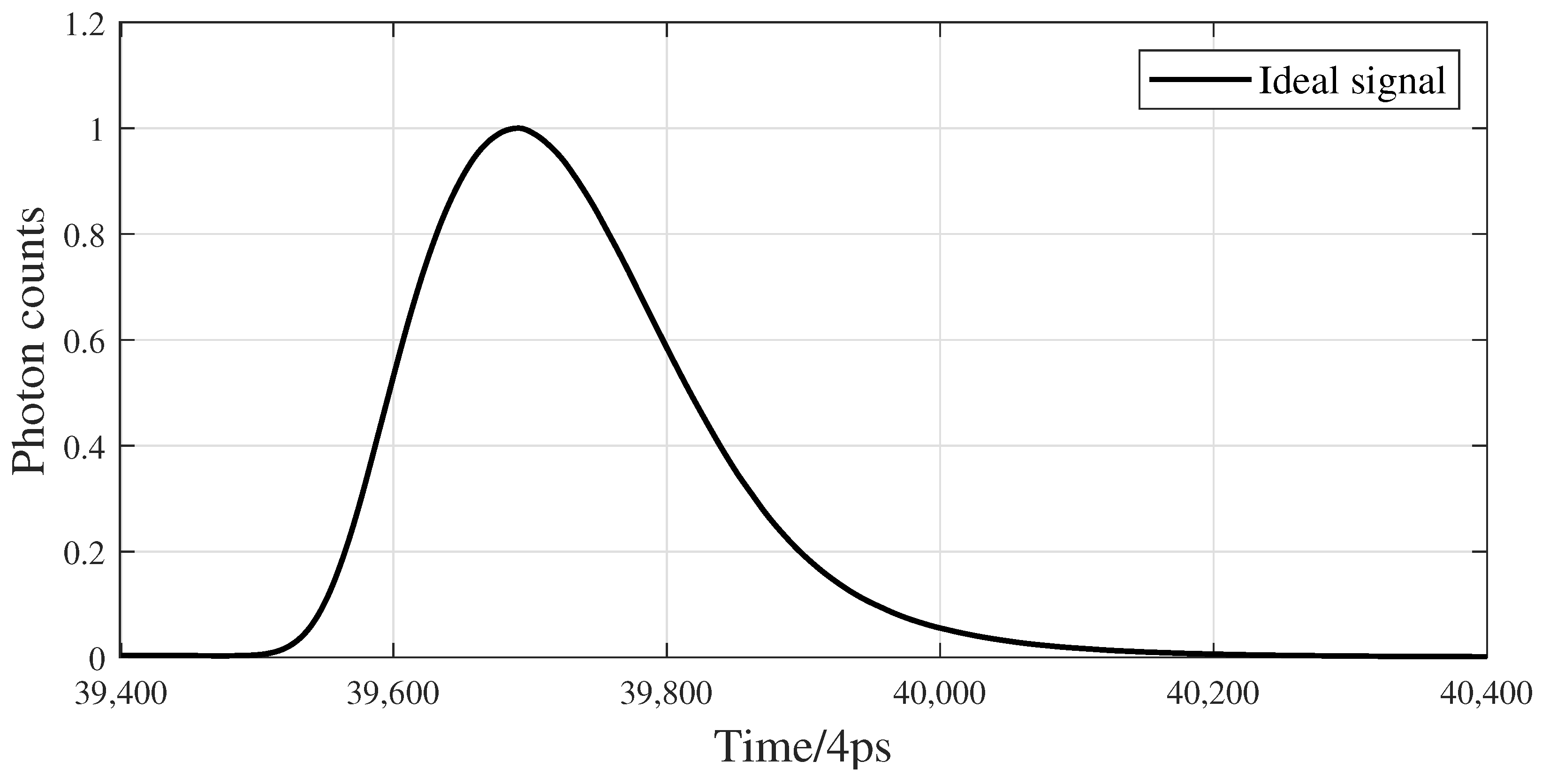
Figure 7 shows the raw data of the first segment of the system return signal from Figure 6. To suppress noise interference in the measured signal, the Variational Mode Decomposition (VMD) algorithm [27] was applied for denoising, as illustrated in Figure 8. The resulting data thus serves as the ideal reference for subsequent waveform fitting experiments.

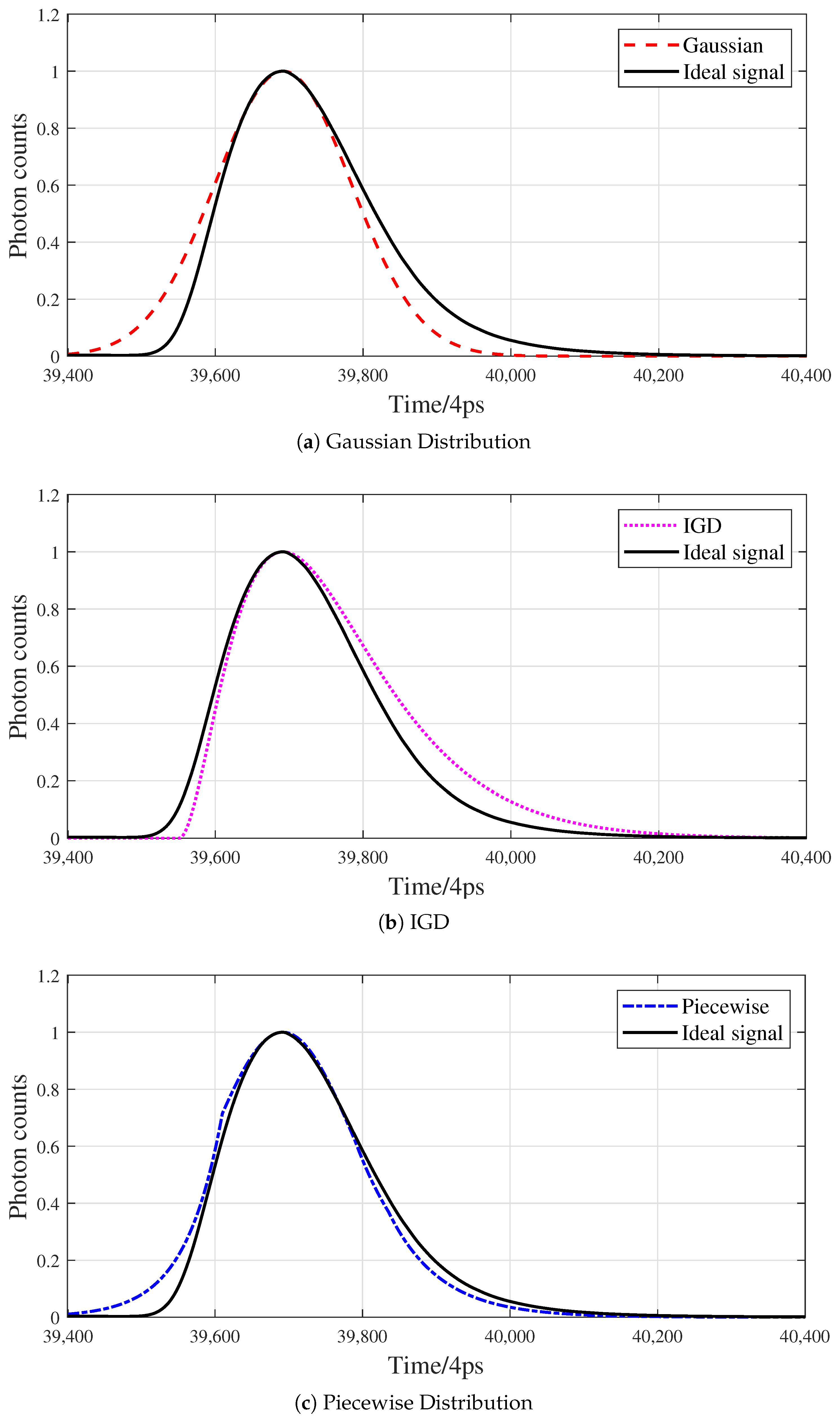
Figure 9 presents the fitting results of the system return signal waveform using the Gaussian model, IGD model, and piecewise model, respectively. Figure 9a depicts the Gaussian model fitting. It is evident that the theoretical waveform deviates substantially from the Gaussian fit, with both the rising and falling edges of the signal inadequately captured. While the Gaussian model, owing to its simplicity and minimal parameters, can approximate the FWHM and peak amplitude of the return signal, it fails to accurately characterize the distinct rise and decay behavior of the measured photon return waveform.

Figure 9b presents the fitting results of the IGD model. Compared to the Gaussian model, the IGD model better represents the rapid rise and slow decay of the LiDAR return signal [19]. Although its fitting performance improves considerably, noticeable discrepancies between the model and the actual waveform remain.

Through theoretical analysis and comparative fitting, it is evident that photon return waveforms from single-photon LiDAR systems are inherently asymmetric. This asymmetry arises fundamentally from the time response of the SPAD detector. While carriers generated in the depletion layer produce a Gaussian-like temporal response, photons reaching the neutral region of the detector prior to carrier generation induce diffusion-related distortions that follow an exponential trend, thereby rendering symmetric Gaussian models inadequate [24,25]. The IGD model improved the fitting accuracy during the slower decay phase but offered limited improvement for the rapid rise segment, making both Gaussian and IGD models insufficient for fully characterizing single-photon LiDAR returns in this study.

While the segment piecewise function model offers higher accuracy, richer features, and greater noise resistance than the Gaussian or IGD models, it also introduces substantial modeling complexity. The large number of parameters means that even minor inaccuracies in parameter estimation can significantly affect the model’s validity and reliability. Additionally, constructing the piecewise function model lacks a unified criterion for selecting the segment count and their functional forms. Consequently, these choices are often made based on the modeler’s experience and subjective judgment. As a result, the piecewise model exhibits high uncertainty and complexity, and its fitting accuracy becomes strongly dependent on the designer’s expertise.

To evaluate the effectiveness of the MBD model proposed in this study for single-photon LiDAR return signal fitting, as well as its superiority over conventional models, a systematic comparative analysis was performed. The MBD model was applied to the waveform matching of system return signals, and its fitting accuracy was assessed using a series of quantitative evaluation metrics. This analysis demonstrates the advantages of the MBD model in accurately representing single-photon photon return waveforms in underwater LiDAR applications.

Figure 9c shows the fitting results of the piecewise model against the theoretical waveform. Compared to the Gaussian and IGD models, the piecewise function achieves substantially improved fitting accuracy, the results are shown in

Table 3. Performance Analysis of The Four Fitting Models.

Model	RMSPE/%	MAPE/%	R-Squared	Pearson Correlation Coefficient
Gaussian	7.26	4.83	0.9530	0.9762
IGD	6.26	4.34	0.9698	0.9848
Piecewise	3.86	2.58	0.9867	0.9933
MBD	1.62	1.04	0.9919	0.9955

. It effectively captures the rapidly rising and gradually decaying trends of the theoretical return signal, although its fitting precision is relatively limited during the ascending phase. This limitation arises primarily from the piecewise function’s reliance on segmentation points. The rising segment is governed by a single piecewise function, whereas the falling segment is modeled using two piecewise functions. As a result, the fitting accuracy for the decay phase exceeds that of the rise phase. The four-segment piecewise function model involves fitting nine parameters. To further enhance precision, more complex piecewise functions have been proposed, which, while improving fitting performance, also increase the number of parameters and consequently the model’s overall complexity.

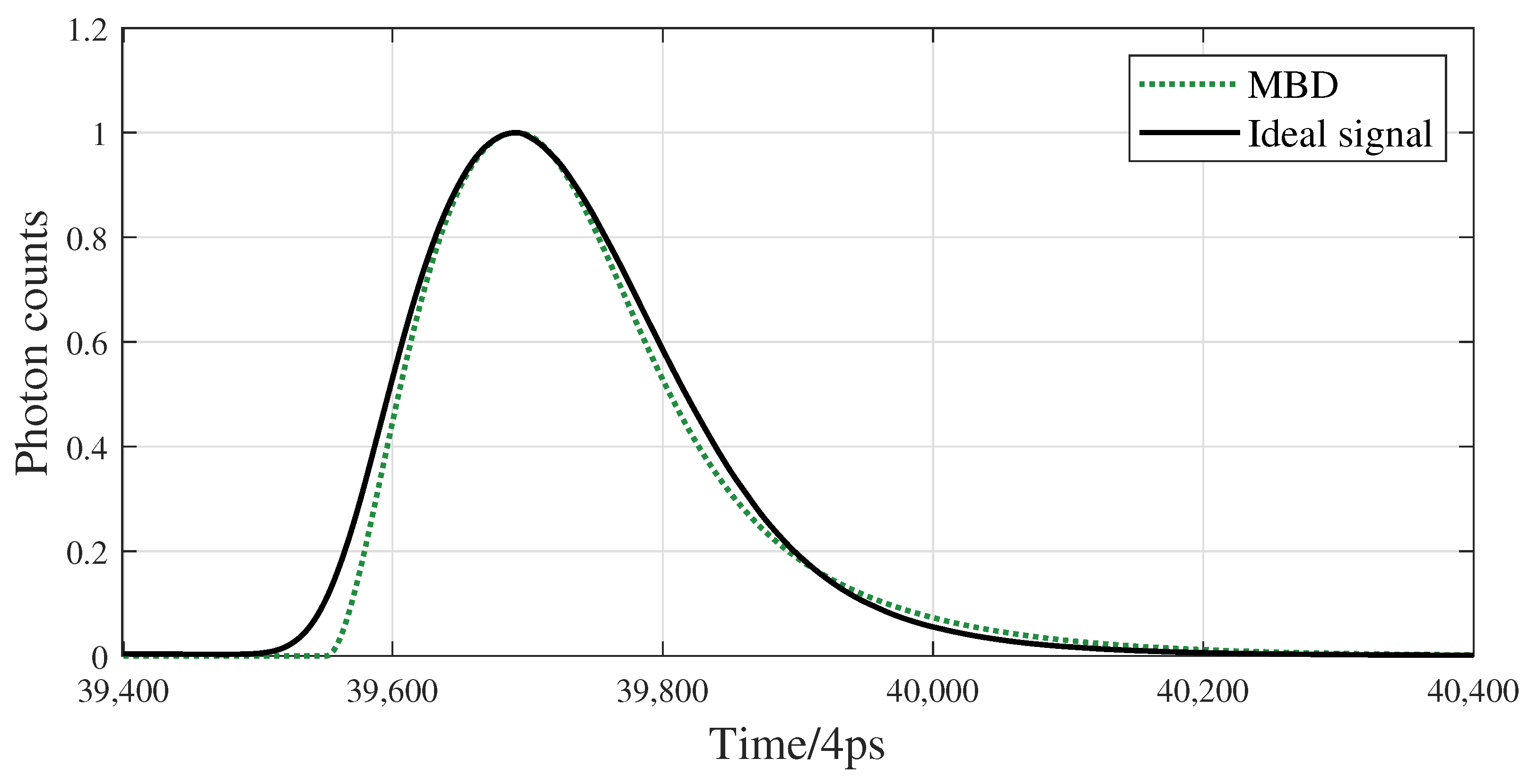
Figure 10 and Table 3 illustrate the fitting performance of the MBD model applied to the theoretical return signals. Compared to the Gaussian and IGD models, the MBD model provides significantly higher fitting accuracy. Notably, in comparison with the four-segment piecewise model, the MBD model achieves a slight improvement in fitting performance despite using fewer parameters (five fewer than the piecewise model). This demonstrates the MBD model’s exceptional ability to balance parameter efficiency with fitting precision, substantially simplifying model complexity while maintaining superior accuracy. These results highlight the efficiency and flexibility of the MBD model in handling complex single-photon return signal analysis.

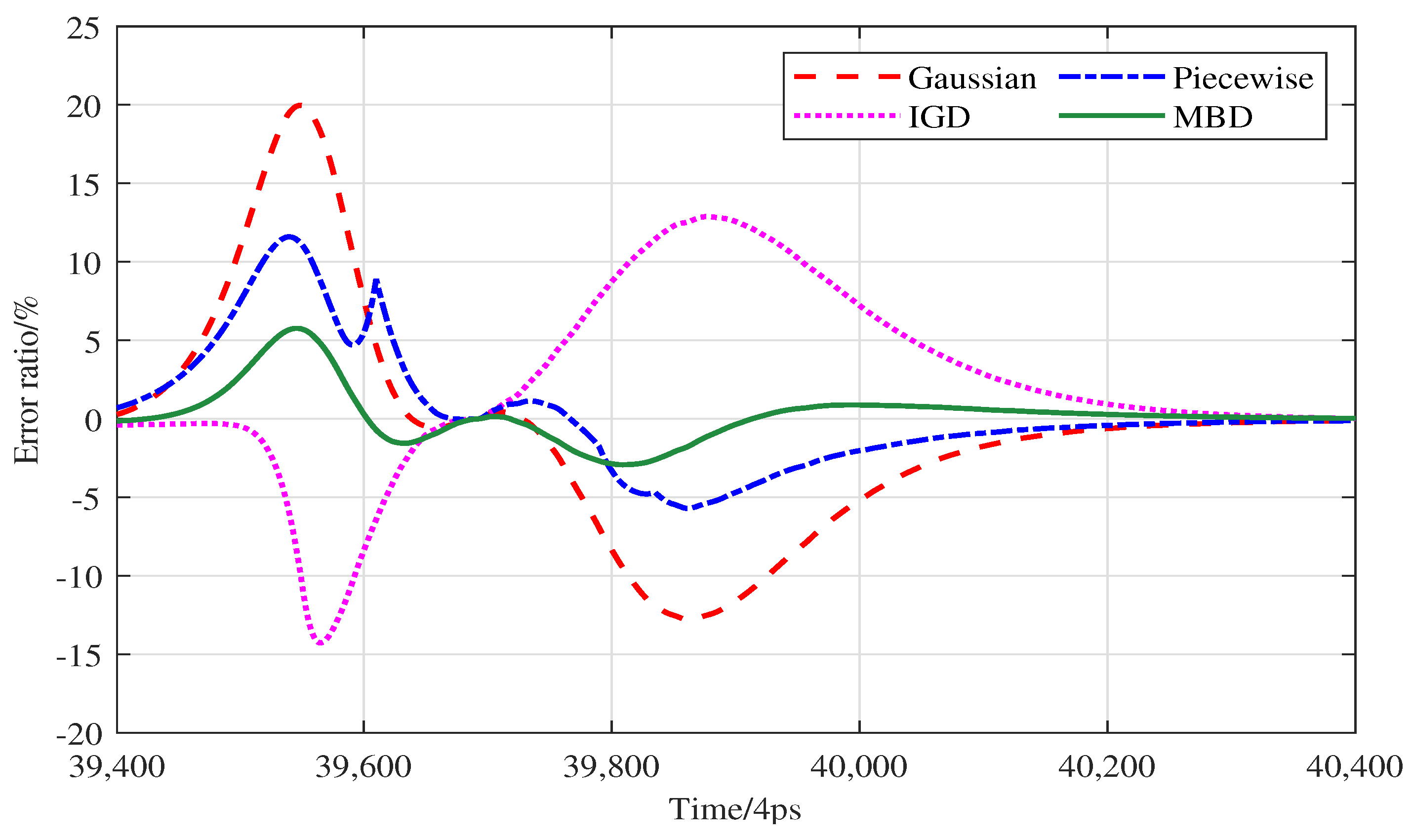
To further illustrate the fitting characteristics of the MBD model, this study compares its performance against the Gaussian, IGD, and four-segment piecewise models. The deviation between each model’s fitted curve and the theoretical return signal was quantified and normalized, and Figure 11 presents the percentage deviation over time for each model. The vertical axis represents the ratio of the normalized deviation of the fitted waveform from the theoretical signal(the denoised reference signal obtained via VMD) to the theoretical signal, providing a clear visual comparison of the relative fitting performance among the models.

To quantitatively evaluate the superiority of the proposed MBD model, several widely accepted statistical metrics were employed, including Root Mean Square Percentage Error (RMSPE), Mean Absolute Percentage Error (MAPE), the coefficient of determination (R-squared), and Pearson’s correlation coefficient. RMSPE and MAPE assess the magnitude of prediction errors, with lower values indicating superior model performance. The R-squared metric evaluates the goodness of fit, ranging from 0 to 1, with higher values reflecting stronger explanatory power and improved fit quality [28,29]. The Pearson correlation coefficient quantifies waveform similarity and the linear relationship between two waveforms [30,31,32]. When r approaches 1, the waveforms are highly positively correlated, indicating very similar shapes; when r approaches −1, the waveforms are negatively correlated, indicating similar shapes but opposite trends; when r approaches 0, there is no significant linear relationship, indicating dissimilar shapes. The mathematical definitions of these evaluation metrics are provided in Equations (10)–(13). Here, $x_i$ and $y_i$ represent the individual values of the ideal signal and the fitted signal at point i, respectively. $\overline{x}$ and $\overline{y}$ denote the mean values of the ideal (reference) signal and the fitted signal, respectively.

$$\mathrm{RMSPE}=\sqrt{{\displaystyle \frac{1}{n}}\sum _{i=1}^n{(x_i-y_i)}^2}\times 100\%$$

(10)

$$\mathrm{MAPE}={\displaystyle \frac{1}{n}}\sum _{i=1}^n|x_i-y_i|\times 100\%$$

(11)

$$R_{squared}=1-{\displaystyle \frac{{\sum }_{i=1}^n{(x_i-y_i)}^2}{{\sum }_{i=1}^n{(y_i-\overline{y})}^2}}$$

(12)

$$r={\displaystyle \frac{{\sum }_{i=1}^n(x_i-\overline{x})(y_i-\overline{y})}{\sqrt{{\sum }_{i=1}^n{(x_i-\overline{x})}^2}\sqrt{{\sum }_{i=1}^n{(y_i-\overline{y})}^2}}}$$

(13)

Using the aforementioned evaluation metrics to quantitatively analyze the fitting performance between the introduced model and the ideal signal, the results are shown in Table 3.

The MBD model achieves the lowest error values among all evaluated models, with RMSPE and MAPE of 1.62 and 1.04, respectively. This demonstrates its superior accuracy compared to alternative approaches. From the perspective of R-squared and Pearson correlation coefficients, all models exhibit relatively high values, indicating good overall agreement with the data. However, the MBD model consistently outperforms the others, yielding an R-squared of 0.9919 and a Pearson correlation coefficient of 0.9955. These results highlight its strong capability for accurately predicting and characterizing single-photon return signals. It should be noted, however, that this improvement in accuracy comes with increased algorithmic complexity relative to simpler models such as the Gaussian and IGD. In contrast, compared to the more complex Piecewise model, the MBD model achieves a reduction in computational cost while still providing competitive—though not drastically superior—accuracy gains. Thus, while the MBD model offers the best overall performance across all evaluated metrics, its practical adoption may involve a trade-off between precision and computational efficiency, depending on the specific application requirements. In summary, across all evaluation criteria, the MBD model demonstrates the best overall performance. It not only minimizes fitting error but also offers robust interpretability of the data, making it a reliable model for describing single-photon return signals in both future research and practical applications.

As shown in Figure 5, laser pulses experience significant temporal broadening when propagating through turbid water. This phenomenon severely degrades the ranging and imaging accuracy of underwater lidar systems. In echo signal processing, the Instrument Response Function (IRF) is typically constructed from long-term accumulated photon returns, and its quality directly affects the accuracy of range estimation obtained through cross-correlation operations. A well-defined IRF enhances ranging precision, whereas a degraded IRF propagates errors into subsequent signal processing, thereby compromising overall system performance. Since the MBD model has been validated as an accurate descriptor of single-photon return signals, it is adopted in this study for correcting underwater target waveforms.

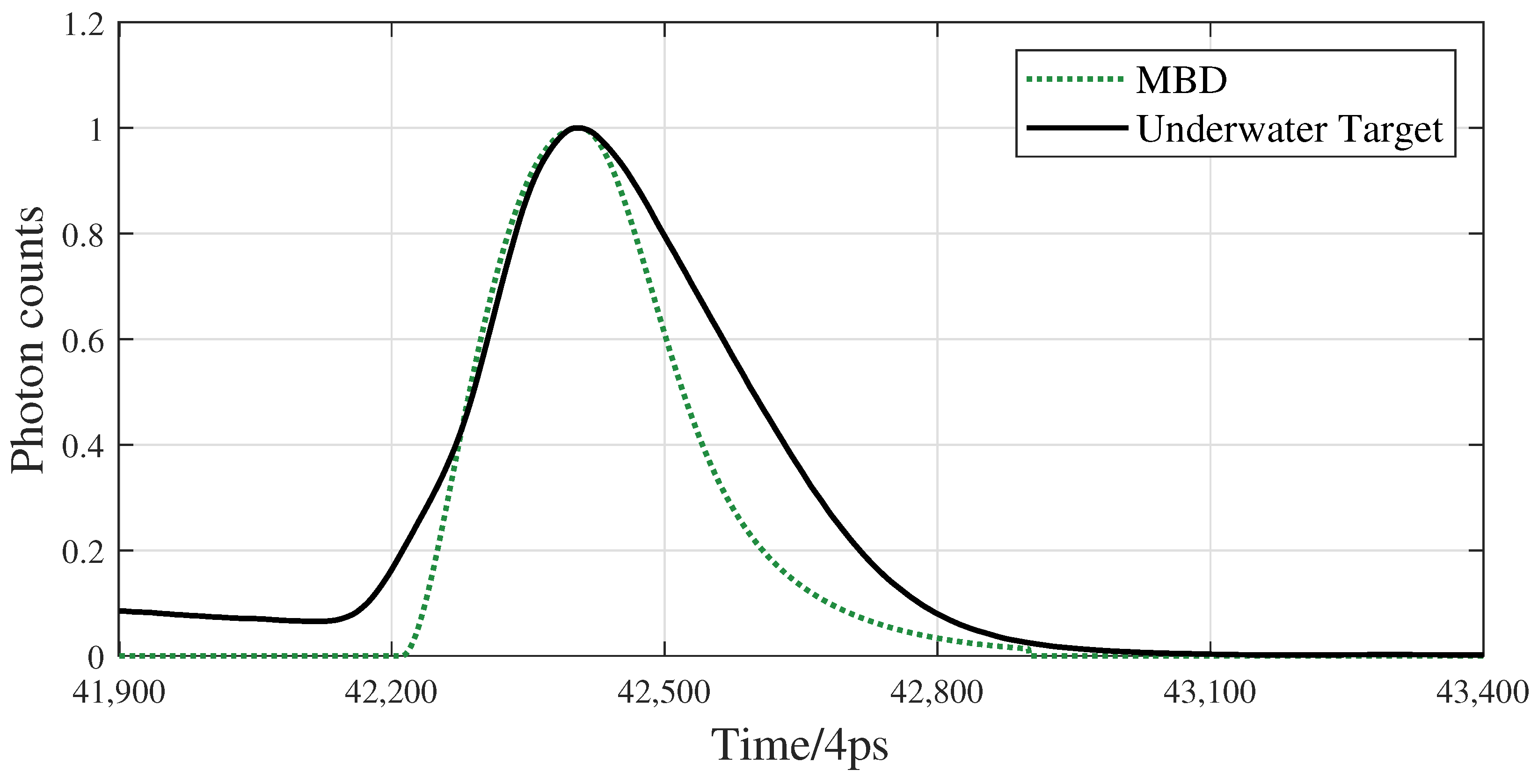
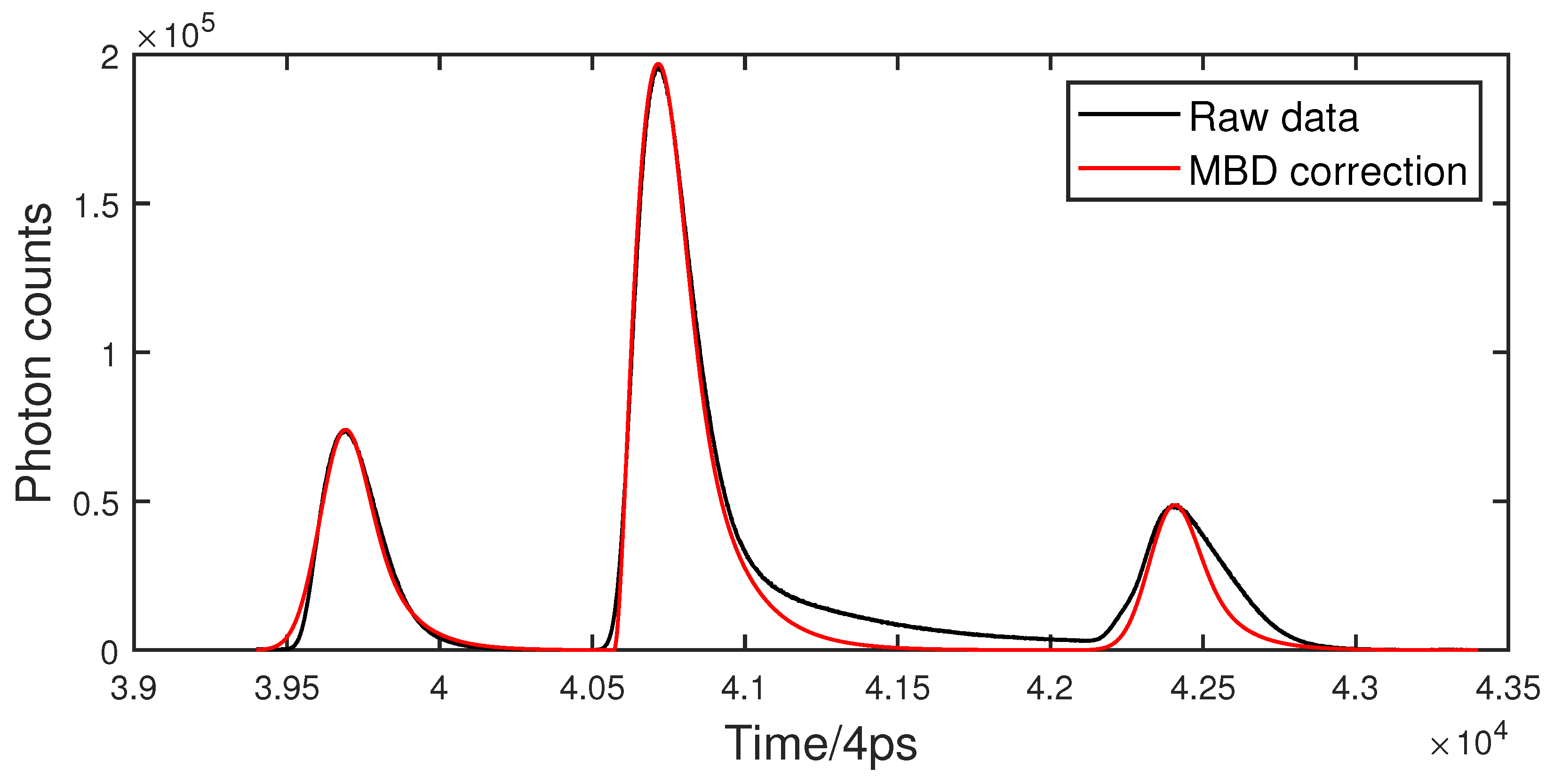
Figure 12 shows the same waveform fitted with the MBD model. Accordingly, the MBD model was applied to correct underwater ranging signals, with the results illustrated in Figure 13. The model-based correction effectively reduces uncertainty in single-photon underwater ranging. Here, “uncertainty reduction” refers to narrowing the search window for range extraction based on the FWHM of the pulse, thereby improving ranging certainty and minimizing error. This approach enables more precise and reliable distance measurements by optimizing the processing of broadened photon return signals.

The experimental setup is identical to that described in Section 3.1. Whereas the previous section focused on single-point ranging, this part extends the analysis to scanning experiments. The target was again a brick, scanned over a 64 × 64 grid (4096 ranging measurements) with a single-point accumulation time of 0.5 s. A two-dimensional scanning mirror was employed to sweep the target, validating the effectiveness of the proposed method. The target surface was raster-scanned using a 64 × 64 grid, covering a physical area of 7.4 cm × 7.4 cm. This configuration results in a center-to-center spatial sampling resolution (distance between adjacent laser points) of approximately 0.12 mm in both the horizontal and vertical directions. The main parameters are summarized in

Table 4. Main parameters of the experiment.

Parameter	Value
Average power	2.85 mW
Pulse repetition frequency	1 MHz
Single-point cumulative time	0.5 s
Image size	$64\times 64$

, with all other conditions consistent with Table 1.

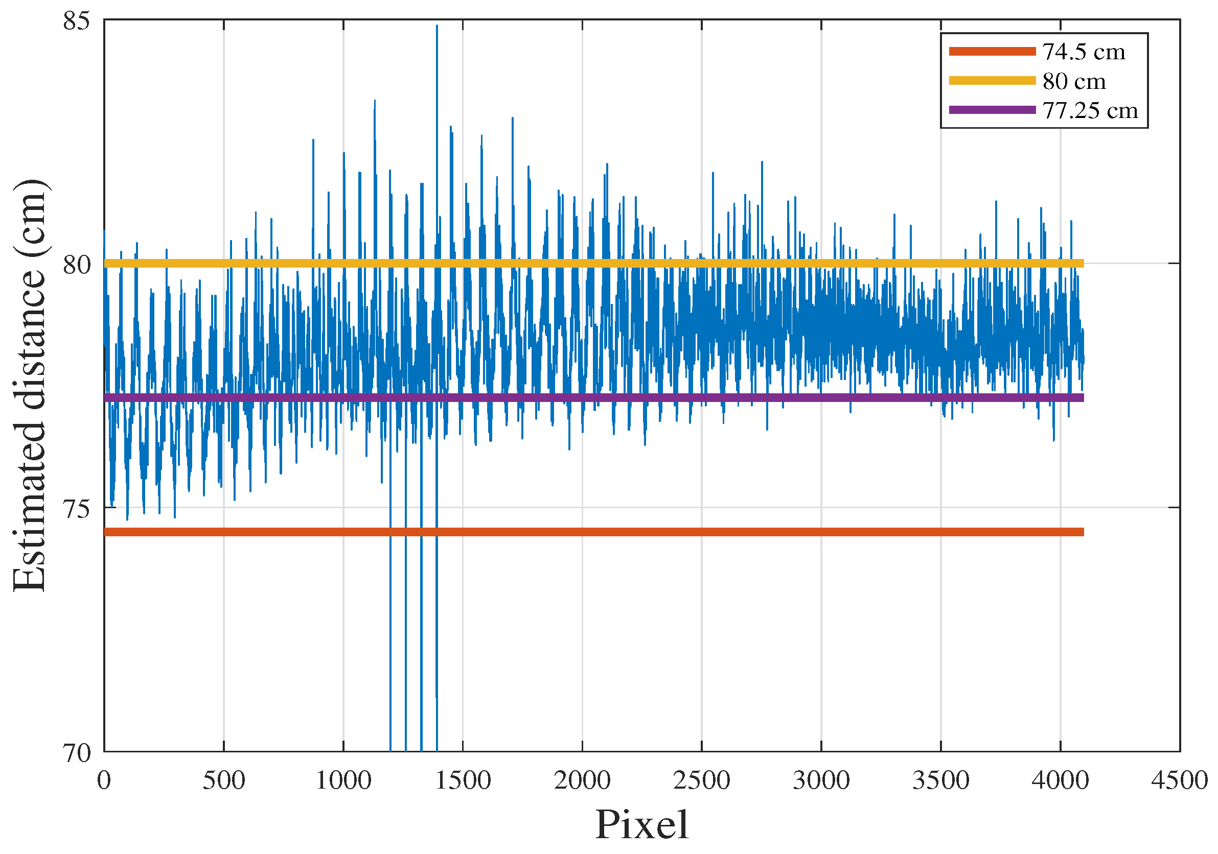
First, statistical analysis was conducted on 4096 sets of distance measurements. Since the measured target was a flat brick and the scanning area was relatively concentrated, the theoretical distance for all 4096 pixel points should be 74.50 cm (corresponding to the distance from the brick surface to the front glass wall). Figure 14 and Figure 15 illustrate the comparison of distance measurements before and after applying MBD correction. To provide clear visual benchmarks, three reference lines are included: the yellow line (top) marks the physical limit of the water tank at 80.00 cm, the purple line (middle) indicates the midpoint of 77.25 cm between the true value and the tank limit, and the orange line (bottom) denotes the true target distance of 74.50 cm. As shown, after applying the MBD model, the measurement results converge more closely toward the true distance. To further assess performance, quantitative evaluation metrics were employed.

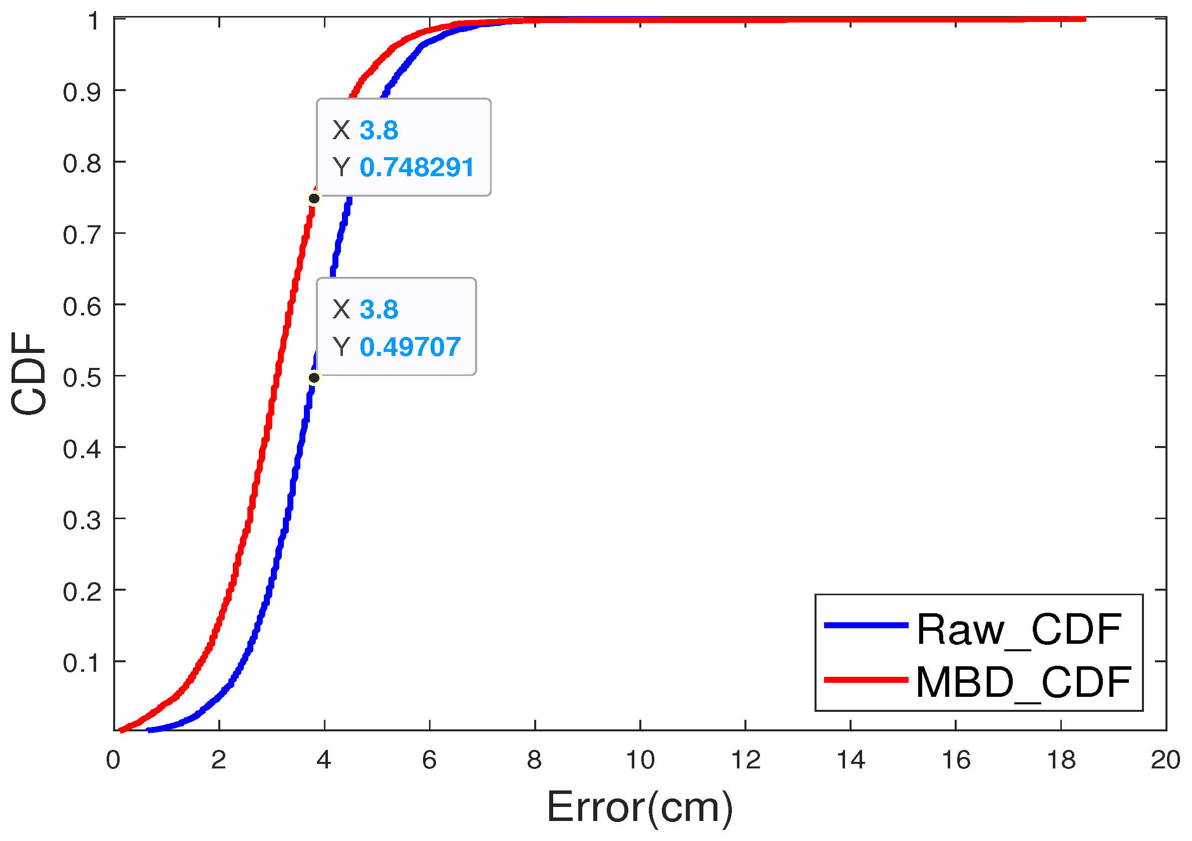
In this section, distance error is evaluated using the Depth Absolute Error (DAE) and the Cumulative Distribution Function (CDF) [33,34]. DAE quantifies the deviation between the estimated and actual depths, as expressed in Equation (14), where $D_{true}$ is the true distance and $D_{est}$ is the estimated distance. Lower DAE values indicate improved accuracy of depth estimation. The CDF reflects the proportion of pixels with DAE values less than or equal to a specified threshold; higher CDF values correspond to lower overall error levels.

$$DAE = |D_{true}-D_{est}|$$

(14)

At an attenuation length of 6.9, the average DAE across the 4096 datasets was 3.82 cm without MBD correction. After applying the MBD correction, the average DAE decreased to 3.15 cm, representing a reduction of 17.54%. These results, validated through 4096 ranging experiments, confirm that MBD correction effectively reduces ranging errors in turbid underwater environments.

Figure 16 further compares the cumulative distribution functions for the datasets before and after correction. The horizontal axis represents absolute distance error, while the vertical axis indicates the cumulative probability of errors below a given threshold. The blue curve corresponds to uncorrected results, and the red curve represents the cumulative distribution function of the corrected data. After MBD correction, the probability of errors below 3.82 cm increased substantially from 49.71% to 74.83%. This demonstrates that the correction reduces error magnitude while improving measurement accuracy. Moreover, the red curve is notably steeper and more concentrated than the blue curve, indicating a narrower error distribution and thus greater robustness and reliability.

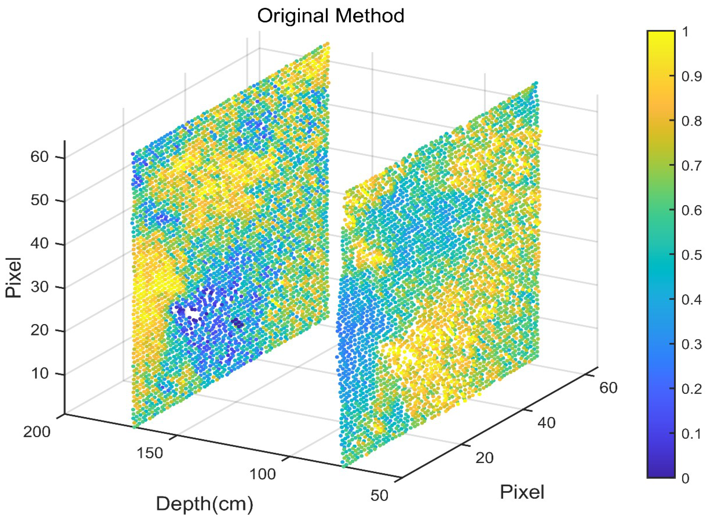
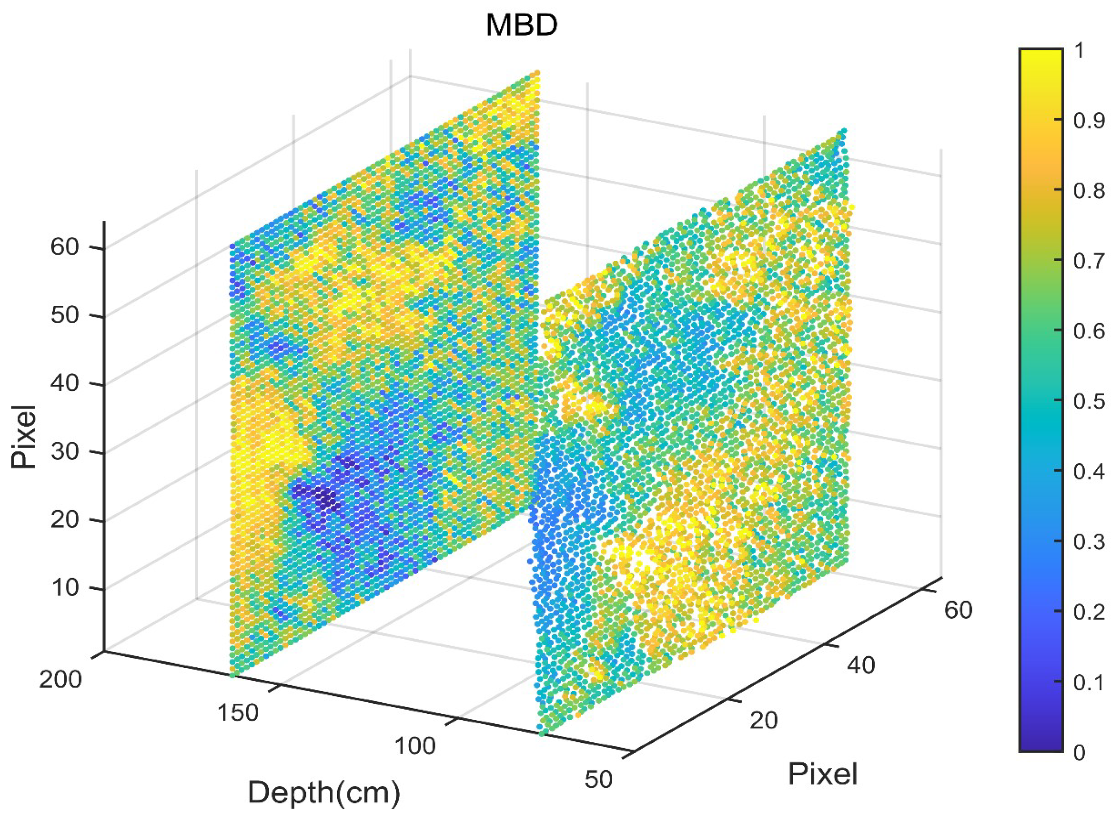
Figure 17 presents the reconstructed 3D point cloud of the scene, where the right plane corresponds to the window of the water tank and the deeper plane represents the submerged target. Figure 18 shows the reconstructed point cloud after MBD correction. The depth information in these point clouds is derived directly from the TCSPC timing grid bins, each with a temporal resolution of 4 ps, corresponding to an underwater spatial resolution of 0.045 cm. By calculating the time-of-flight difference between bins associated with the two planes, the relative distance between the target and the tank wall was obtained. The color scale, consistent in both figures, indicates the dimensionless relative reflectivity for each pixel, calculated as its photon event count normalized by the maximum event count across the entire 4096-pixel dataset.The comparison between Figure 17 and Figure 18 clearly demonstrates that the MBD correction improves the accuracy of the reconstructed 3D point cloud.

4.2. Discussion and Limitations

It is important to acknowledge the current limitations of the proposed method. Firstly, the parameter selection for the MBD model partially relies on manual/empirical tuning, lacking a mechanism for rapid, fully adaptive optimization under varying underwater conditions. This dependence may affect the model’s generalization capability and ease of deployment in uncharacterized or highly dynamic environments. Secondly, the validation in this study has been conducted exclusively on a system with a single-point detector combined with a scanning galvanometer. The method’s performance and potential integration challenges within array-detector systems, which are pivotal for achieving faster frame rates and wider fields of view, remain to be investigated and validated. Additionally, this study did not conduct experimental validation under different turbidity levels; future work will validate this algorithm under varying water turbidity conditions.

Although this study demonstrates that the proposed MBD model achieves higher accuracy, a formal analysis of the trade-off between model complexity (e.g., number of parameters, computational cost) and performance gains has yet to be conducted. Determining the optimal complexity threshold for practical applications remains a critical issue. Future work will systematically analyze the trade-off between complexity and performance.

Furthermore, while the current analysis validates the model’s core performance, a more comprehensive exploitation of the experimental dataset is planned. Future work will pursue two interconnected directions: First, a systematic post-analysis to mine deeper insights from existing data, such as detailed error source attribution and performance boundaries. Second, the integration of statistical analysis of residual errors (e.g., fitting to theoretical distributions) with expanded performance evaluations across varying attenuation lengths and scenarios. Together, this will build a more complete predictive error model and a thorough understanding of the system’s behavior.

This paper primarily focuses on measurement errors in distance estimation and does not delve deeply into photon detection probability (reflectivity), which may overlook several critical aspects. Future work will integrate detection probability to refine the model.

5. Conclusions

To address the challenge of pulse broadening in underwater environments—caused by medium properties and environmental factors—which degrades ranging accuracy, this paper focuses on echo feature extraction techniques for underwater LiDAR systems. The objective is to enhance detection performance by developing a more accurate model of underwater signal echoes. First, several classical and widely used LiDAR echo models are introduced, including the Gaussian distribution model, the IGD distribution model, and the four-segment piecewise function model, with an in-depth analysis of their respective characteristics. By fitting these traditional models to measured single-photon echo data, a solid theoretical basis is established for subsequent research.

Recognizing the limitations of conventional models in representing echoes in complex underwater conditions, this study proposes a photon-counting echo signal model based on a Modified Biexponential Distribution (MBD). This model combines the strengths of both biexponential and Gaussian distributions, enabling more accurate characterization of the sharp rising edge and the gradual decay observed in single-photon detection echo signals. The effectiveness of the MBD model is validated through underwater ranging and imaging experiments. At an attenuation length of 6.9, the average Depth Absolute Error (DAE) decreased from 3.82 cm to 3.15 cm, corresponding to a 17.54% reduction. Moreover, the probability of achieving a DAE below 3.82 cm increased significantly from 49.71% to 74.83%. These results demonstrate a substantial improvement in ranging accuracy, confirming the practicality and robustness of the proposed model.

Future research will focus on several promising directions. First, we plan to explore adaptive or learning-based variants of the MBD model, enabling it to automatically adjust parameters in response to changes in water turbidity. Second, the integration of the algorithm onto array detectors will be investigated to further reduce ranging errors caused by the time-lag inherent in scanning imaging. Finally, to systematically validate and extend the model’s generalizability—which is grounded in the physical principles of SPAD response and radiative transfer—future work will test its performance across a broader range of scenarios, including diverse water bodies, longer distances, varying target materials, and more dynamic or extreme underwater environments. This will help assess the model’s practical limits and deployment potential.

References

1. Shen, Y.; Zhao, C.; Liu, Y.; Wang, S.; Huang, F. Underwater optical imaging: Key technologies and applications review. IEEE Access 2021, 9, 85500–85514. [Google Scholar] [CrossRef]
2. Sun, K.; Cui, W.; Chen, C. Review of underwater sensing technologies and applications. Sensors 2021, 21, 7849. [Google Scholar] [CrossRef] [PubMed]
3. Jaffe, J.S. Underwater optical imaging: The past, the present, and the prospects. IEEE J. Ocean. Eng. 2014, 40, 683–700. [Google Scholar] [CrossRef]
4. Li, Z.P.; Ye, J.T.; Huang, X.; Jiang, P.Y.; Cao, Y.; Hong, Y.; Yu, C.; Zhang, J.; Zhang, Q.; Peng, C.Z.; et al. Single-photon imaging over 200 km. Optica 2021, 8, 344–349. [Google Scholar] [CrossRef]
5. Li, Z.P.; Huang, X.; Cao, Y.; Wang, B.; Li, Y.H.; Jin, W.; Yu, C.; Zhang, J.; Zhang, Q.; Peng, C.Z.; et al. Single-photon computational 3D imaging at 45 km. Photonics Res. 2020, 8, 1532–1540. [Google Scholar] [CrossRef]
6. Yu, Y.; Wang, Z.; Chen, C.; Zhang, E.; Li, H.; Yu, C.; Wang, X.; Li, X.; Xue, B.; Zhuang, Q.; et al. 3D imaging of underwater scanning photon counting lidar based on multiscale spatio-temporal resolution. Opt. Express 2025, 33, 4463–4473. [Google Scholar] [CrossRef]
7. Maccarone, A.; Acconcia, G.; Steinlehner, U.; Labanca, I.; Rech, I.; Buller, G.S. Underwater time of flight depth imaging using an asynchronous linear single photon avalanche diode detector array. In Proceedings of the Emerging Imaging and Sensing Technologies for Security and Defence V; and Advanced Manufacturing Technologies for Micro-and Nanosystems in Security and Defence III; SPIE: Bellingham, WA, USA, 2020; Volume 11540, pp. 102–108. [Google Scholar]
8. Maccarone, A.; Drummond, K.; McCarthy, A.; Steinlehner, U.K.; Petillot, Y.R.; Henderson, R.K.; Altmann, Y.; Buller, G.S. Real-time underwater single-photon three-dimensional imaging. In Proceedings of the Emerging Imaging and Sensing Technologies for Security and Defence VII; SPIE: Bellingham, WA, USA, 2022; Volume 12274, p. 1227403. [Google Scholar]
9. Shangguan, M.; Li, Y.; Mo, Y.; Wang, J.; Huang, T. Compact underwater single-photon imaging lidar. Opt. Lett. 2025, 50, 1957–1960. [Google Scholar] [CrossRef]
10. Rong, T.; Wang, Y.; Zhu, Q.; Wang, C.; Zhang, Y.; Li, J.; Zhou, Z.; Luo, Q. Sequential Multimodal Underwater Single-Photon Lidar Adaptive Target Reconstruction Algorithm Based on Spatiotemporal Sequence Fusion. Remote Sens. 2025, 17, 295. [Google Scholar] [CrossRef]
11. de Dios Carbajal, A.; Buller, G.S.; Maccarone, A. Single-photon depth imaging for underwater target discrimination. In Proceedings of the Advanced Photon Counting Techniques XIX; SPIE: Bellingham, WA, USA, 2025; Volume 13448, p. 134480H. [Google Scholar]
12. Adeoluwa, O.; Schnier, K.; Coldwell, C.; Swakshar, A.; Kung, P.; Gurbuz, S.; Kim, M. End-to-end underwater object recognition using multipolarization image fusion with single-photon LiDAR. In Proceedings of the Signal Processing, Sensor/Information Fusion, and Target Recognition XXXIV; SPIE: Bellingham, WA, USA, 2025; Volume 13479, pp. 269–280. [Google Scholar]
13. Maccarone, A.; Drummond, K.; McCarthy, A.; Steinlehner, U.K.; Tachella, J.; Garcia, D.A.; Pawlikowska, A.; Lamb, R.A.; Henderson, R.K.; McLaughlin, S.; et al. Submerged single-photon LiDAR imaging sensor used for real-time 3D scene reconstruction in scattering underwater environments. Opt. Express 2023, 31, 16690–16708. [Google Scholar] [CrossRef]
14. Maccarone, A.; Della Rocca, F.M.; McCarthy, A.; Henderson, R.; Buller, G.S. Three-dimensional imaging of stationary and moving targets in turbid underwater environments using a single-photon detector array. Opt. Express 2019, 27, 28437–28456. [Google Scholar] [CrossRef]
15. Wang, J.; Hao, W.; Chen, S.; Xie, M.; Li, X.; Shi, H.; Feng, X.; Su, X. Underwater single photon profiling under turbulence and high attenuation environment. IEEE Geosci. Remote Sens. Lett. 2024, 21, 1–5. [Google Scholar] [CrossRef]
16. Wang, J.; Hao, W.; Chen, S.; Zhang, Z.; Xu, W.; Xie, M.; Zhu, W.; Su, X. Underwater single photon 3D imaging with millimeter depth accuracy and reduced blind range. Opt. Express 2023, 31, 30588–30603. [Google Scholar] [CrossRef]
17. Richards, M.A. Fundamentals of Radar Signal Processing; McGraw-Hill Education: Columbus, OH, USA, 2014. [Google Scholar]
18. Lindell, D.B.; O’Toole, M.; Wetzstein, G. Single-photon 3D imaging with deep sensor fusion. ACM Trans. Graph. 2018, 37, 1–12. [Google Scholar] [CrossRef]
19. Zhang, Z.; Chen, S.; Wang, J.; Ma, C.; Su, X. Precision Improvement of Underwater Single Photon Imaging Based on Model Matching. IEEE Photonics Technol. Lett. 2023, 35, 253–256. [Google Scholar] [CrossRef]
20. Hua, K.; Liu, B.; Fang, L.; Wang, H.; Chen, Z.; Luo, J. Correction of range walk error for underwater photon-counting imaging. Opt. Express 2020, 28, 36260–36273. [Google Scholar] [CrossRef] [PubMed]
21. Steinvall, O.K.; Carlsson, T. Three-dimensional laser radar modeling. In Proceedings of the Laser Radar Technology and Applications VI; SPIE: Bellingham, WA, USA, 2001; Volume 4377, pp. 23–34. [Google Scholar]
22. Hernandez-Marin, S.; Wallace, A.M.; Gibson, G.J. Bayesian analysis of lidar signals with multiple returns. IEEE Trans. Pattern Anal. Mach. Intell. 2007, 29, 2170–2180. [Google Scholar] [CrossRef] [PubMed]
23. Pellegrini, S.; Buller, G.S.; Smith, J.M.; Wallace, A.M.; Cova, S. Laser-based distance measurement using picosecond resolutiontime-correlated single-photon counting. Meas. Sci. Technol. 2000, 11, 712. [Google Scholar] [CrossRef]
24. Greeley, A.P.; Neumann, T.A.; Kurtz, N.T.; Markus, T.; Martino, A.J. Characterizing the system impulse response function from photon-counting LiDAR data. IEEE Trans. Geosci. Remote Sens. 2019, 57, 6542–6551. [Google Scholar] [CrossRef]
25. Rapp, J.; Dawson, R.M.; Goyal, V.K. Dithered depth imaging. Opt. Express 2020, 28, 35143–35157. [Google Scholar] [CrossRef]
26. Gu, Z.; Ying, Y.L.; Yan, B.Y.; Wang, H.F.; He, P.G.; Long, Y.T. Exponentially modified Gaussian relevance to the distributions of translocation events in nanopore-based single molecule detection. Chin. Chem. Lett. 2014, 25, 1029–1032. [Google Scholar] [CrossRef]
27. Wang, S.C.; Su, X.Q.; Zhu, W.H.; Chen, S.M.; Zhang, Z.Y.; Xu, W.H.; Wang, D.J. A time-correlated single photon counting signal denoising method based on elastic variational mode extraction. ACTA Phys. Sin. 2021, 70. [Google Scholar] [CrossRef]
28. Hong, Y.; Liu, S.; Li, Z.P.; Huang, X.; Jiang, P.; Xu, Y.; Wu, C.; Zhou, H.; Zhang, Y.C.; Ren, H.L.; et al. Airborne single-photon LiDAR towards a small-sized and low-power payload. Optica 2024, 11, 612–618. [Google Scholar] [CrossRef]
29. Chicco, D.; Warrens, M.J.; Jurman, G. The coefficient of determination R-squared is more informative than SMAPE, MAE, MAPE, MSE and RMSE in regression analysis evaluation. PeerJ Comput. Sci. 2021, 7, e623. [Google Scholar] [CrossRef] [PubMed]
30. Teng, T.P.; Chen, W.J. Using Pearson correlation coefficient as a performance indicator in the compensation algorithm of asynchronous temperature-humidity sensor pair. Case Stud. Therm. Eng. 2024, 53, 103924. [Google Scholar] [CrossRef]
31. Gong, H.; Li, Y.; Zhang, J.; Zhang, B.; Wang, X. A new filter feature selection algorithm for classification task by ensembling pearson correlation coefficient and mutual information. Eng. Appl. Artif. Intell. 2024, 131, 107865. [Google Scholar] [CrossRef]
32. Yu, H.; Hutson, A.D. Inferential procedures based on the weighted Pearson correlation coefficient test statistic. J. Appl. Stat. 2024, 51, 481–496. [Google Scholar] [CrossRef]
33. Tobin, R.; Altmann, Y.; Ren, X.; McCarthy, A.; Lamb, R.A.; McLaughlin, S.; Buller, G.S. Comparative study of sampling strategies for sparse photon multispectral lidar imaging: Towards mosaic filter arrays. J. Opt. 2017, 19, 094006. [Google Scholar] [CrossRef]
34. Ren, X.; Altmann, Y.; Tobin, R.; Mccarthy, A.; Mclaughlin, S.; Buller, G.S. Wavelength-time coding for multispectral 3D imaging using single-photon LiDAR. Opt. Express 2018, 26, 30146–30161. [Google Scholar] [CrossRef]
Figure 1. Workflow of the proposed underwater single-photon ranging method based on IRF calibration and MBD modeling.
Remotesensing 18 00489 g001
Figure 2. Schematicdiagram of the experimental setup.
Remotesensing 18 00489 g002
Figure 3. Experimental scenario. (a) Main View. (b) Top View.
Remotesensing 18 00489 g003
Figure 5. Comparison of Laser Underwater Transmission Scattering. (a) Clear water environment. (b) Turbid water environment.
Remotesensing 18 00489 g005
Figure 6. Effective Information Intercept Segment.
Remotesensing 18 00489 g006
Figure 7. Original effective section of the optical system’s return.
Remotesensing 18 00489 g007
Figure 8. The ideal signal after denoising the signal in Figure 7.
Remotesensing 18 00489 g008
Figure 9. Diagram comparing ordinary model fits to theoretical signals. (a) Gaussian model, (b) modified Gaussian model, (c) piecewise function model.
Remotesensing 18 00489 g009
Figure 10. Comparison of MBD Model Fitting and Reconstruction for Theoretical Signals.
Remotesensing 18 00489 g010
Figure 11. Comparisonresults of the percentage deviation of each model from the theoretical value with time.
Remotesensing 18 00489 g011
Figure 12. Underwater target signals corrected using MBD models.
Remotesensing 18 00489 g012
Figure 13. Comparison of the original (raw) photon counting histogram and the histogram corrected by the MBD model.
Remotesensing 18 00489 g013
Figure 14. Statistical results of 4096 sets of ranging data without MBD modeling.
Remotesensing 18 00489 g014
Figure 15. Statistical results of 4096 sets of ranging data after correction by the MBD model.
Remotesensing 18 00489 g015
Figure 16. The cumulative distribution function (CDF) plots of the two data sets.
Remotesensing 18 00489 g016
Figure 17. Three-dimensional imaging point cloud of Figure 3 underwater targets.
Remotesensing 18 00489 g017
Figure 18. Three-dimensional imaging point cloud corrected via MBD of Figure 3 underwater targets.
Remotesensing 18 00489 g018