Article

Multi-Sensor Hybrid Modeling of Urban Solar Irradiance via Perez–Ineichen and Deep Neural Networks

by
Zeenat Khadim Hussain
1,
Congshi Jiang
1 and
Rana Waqar Aslam
2,*
1
School of Remote Sensing and Information Engineering, Wuhan University, Wuhan 430079, China
2
State Key Laboratory of Information Engineering in Surveying, Mapping and Remote Sensing (LIESMARS), Wuhan University, Wuhan 430079, China
*
Author to whom correspondence should be addressed.
Remote Sens. 2026, 18(1), 33; https://doi.org/10.3390/rs18010033
Submission received: 2 November 2025 / Revised: 16 December 2025 / Accepted: 16 December 2025 / Published: 23 December 2025

Highlights

What are the main findings?
  • The combination of the Perez–Ineichen (PI) model with a Deep Neural Network (DNN) for accurate urban solar irradiance (USI) prediction in Wuhan using high-resolution Sentinel-2 data.
  • Spectral-band selection and attention mechanism techniques are utilized to enhance the accuracy of solar irradiance prediction.
What are the implications of the main findings?
  • Comprehensive error analysis is conducted to identify the limitations of irradiance predictions particularly under cloud-affected conditions and to propose directions for future improvements.
  • Validation using hyperspectral imagery: Global Horizontal Irradiance (GHI) and Direct Normal Irradiance (DNI) maps produced by the model are compared with reference hyperspectral GHI maps derived from Sentinel-2 imagery to assess accuracy and reliability.

Abstract

An accurate estimate of sun irradiance is important for solar energy management in urban areas with complicated atmospheric conditions. The urban solar irradiance (USI) can be predictively researched with a variety of models; however, basing this entirely on one model often leads to other important conditions being omitted. A hybrid framework is suggested in this study, integrating the Perez–Ineichen PI model with a Deep Neural Network (DNN) model for predicting USI in Wuhan, China. The PI model predicts clear-sky irradiance labels based on atmospheric parameters normalized against the National Solar Radiation Database for greater accuracy. The model is trained on the Clear Sky Index with real-time atmospheric parameters gained from ground station measurements and satellite images. Following correlation analysis using bands from Sentinel-2 to find suitable bands for the model, the algorithm was prepared for atmospheric parameters, including cloud cover, aerosol concentration, and surface reflectance, all of which impact solar radiation. The architecture incorporates attention methods for important atmospheric parameters and skip connections for greater training stability. Results from the Deep Neural Network-Selected bands (DNN-S) and Deep Neural Network-All bands (DNN-A) models gave different performances, with the DNN-S model yielding better accuracy with a RMSE of 69.49 W/m2 clear-sky, 87.60 W/m2 cloudy-sky, and 72.57 W/m2 all-sky. The results were validated using hyperspectral imagery, along with cloud mask, solar area, and surface albedo-derived products, confirming that the USI estimates are supported by the high precision and consistency of Sentinel-2-derived irradiance estimates.

1. Introduction

Effective solar energy planning requires a thorough assessment of solar irradiance, which is even more crucial in urban environments, where the reflectance of surfaces, combined with dust and cloudiness, has a significant impact on solar radiation [1,2,3]. Solar energy is an untapped, renewable, and flexible energy source of great potential [4]. In consequence, various countries have developed national energy policies and plans directed at complying with internationally agreed climate objectives [4]. The problems of accurate estimation of solar irradiance rise with expanding urban areas [5,6]. The difficulty of solar energy planning is increased by the diversity of the meteorological conditions [7]. Urban solar irradiance (USI) is difficult to predict accurately because of factors that typical models are unable to fully account for, such as surface variations including building, road, vegetations, and changing weather conditions, for instance cloud cover and pollution. These elements reduce the accuracy of solar irradiance forecasts made with single-model methods. To address these challenges, this study proposes a hybrid model that combines DNNs with the PI model. The hybrid model improves the precision and flexibility of USI forecasts in a variety of urban settings, such as clear-, cloudy-, and all-sky situations, by combining high-resolution satellite data, spectral band selection, and real-time atmospheric characteristics. Although the PI model and other traditional methods of estimating solar irradiance permitted an understanding of clear-sky conditions, the complexity of urban areas makes them incapable of providing satisfactory results [8,9]. Satellite irradiance algorithms may conveniently be separated into statistical and physical model classes [10,11,12]. The physical model includes Heliosat-4 and the National Solar Radiation Database (NSRDB), enabling the provision of model output and the physical examination of the mechanisms controlling the interactions between solar radiation and atmospheric substances [13]. The new developments in modern remote sensing, particularly with the availability of satellite data from systems such as the GOES system [14,15,16,17,18], will permit more exact estimates of solar irradiance [14,15,16,17,18]. With the availability of high geographical and temporal resolution satellite data and the recent rapid advancements in machine learning techniques, particularly deep learning, this issue has drawn attention [19,20,21]. This work provides a hybrid model aimed at overcoming current deficiencies by the use of the PI model and a DNN. This hybrid model gives a more exact and uniform estimate of USI through the use of authentic real-time atmospheric data and satellite data. By taking into account important variables such as aerosol density, atmospheric turbidity (cloud optical thickness), surface temperature, and altitude, the PI model is utilized to estimate clear-sky irradiance [22,23]. The relevant data are subject to normalization with the NRDB data for clear-sky conditions, which results in more uniform conditions [24,25]. Also, the DNN analysis yields correlated important values for the surface reflectance spectrum, which are estimated with Pearson correlation analysis to record which spectral indices have the highest correlation with irradiance values [26,27,28]. Using real-time atmospheric variables such as the Clear-Sky Index (CSI) and other elements, the novel method improves irradiance prediction by integrating a DNN to increase predictive accuracy [29]. The use of the Sentinel-2 platform is made to provide the user with timely estimates of spatial changes in USI in cities. Further improvements to the DNN architecture are realized with the application of advanced techniques, such as attention mechanisms that help focus on the most significant atmospheric parameters and skip connections that improve model training as well as overall performance [30]. These advancements enable the model to more effectively capture intricate non-linear correlations in the data, which helps it produce feasible, accurate, and trustworthy estimates of solar irradiance in urban settings [31]. Additionally, the use of hyperspectral imagery for irradiance estimation provides a powerful means of validating model predictions (see Table A1). This dual-purpose usage allows the joint application of traditional models with machine learning techniques to increase accuracy and thereby make the framework a usable method of solar energy-dependent planning in realistic, complex urban environments. Primary highlights from this study include:
  • The combination of PI with DNN for accurate USI predictions in Wuhan, utilizing high-resolution Sentinel-2 data.
  • Spectral-band selection and attention mechanism methods are utilized to aid in improved solar irradiance prediction.
  • Error analysis is being performed to understand the shortcomings of irradiance predictions, especially under cloud conditions, and offers future improvement methodologies.
  • Validation via hyperspectral imagery: Global Horizontal Irradiance (GHI) and Direct Normal Irradiance (DNI) maps produced by model outputs compare with genuine hyperspectral GHI maps from Sentinel-2 imagery for accuracy and reliability of model predictions.

2. Methodology

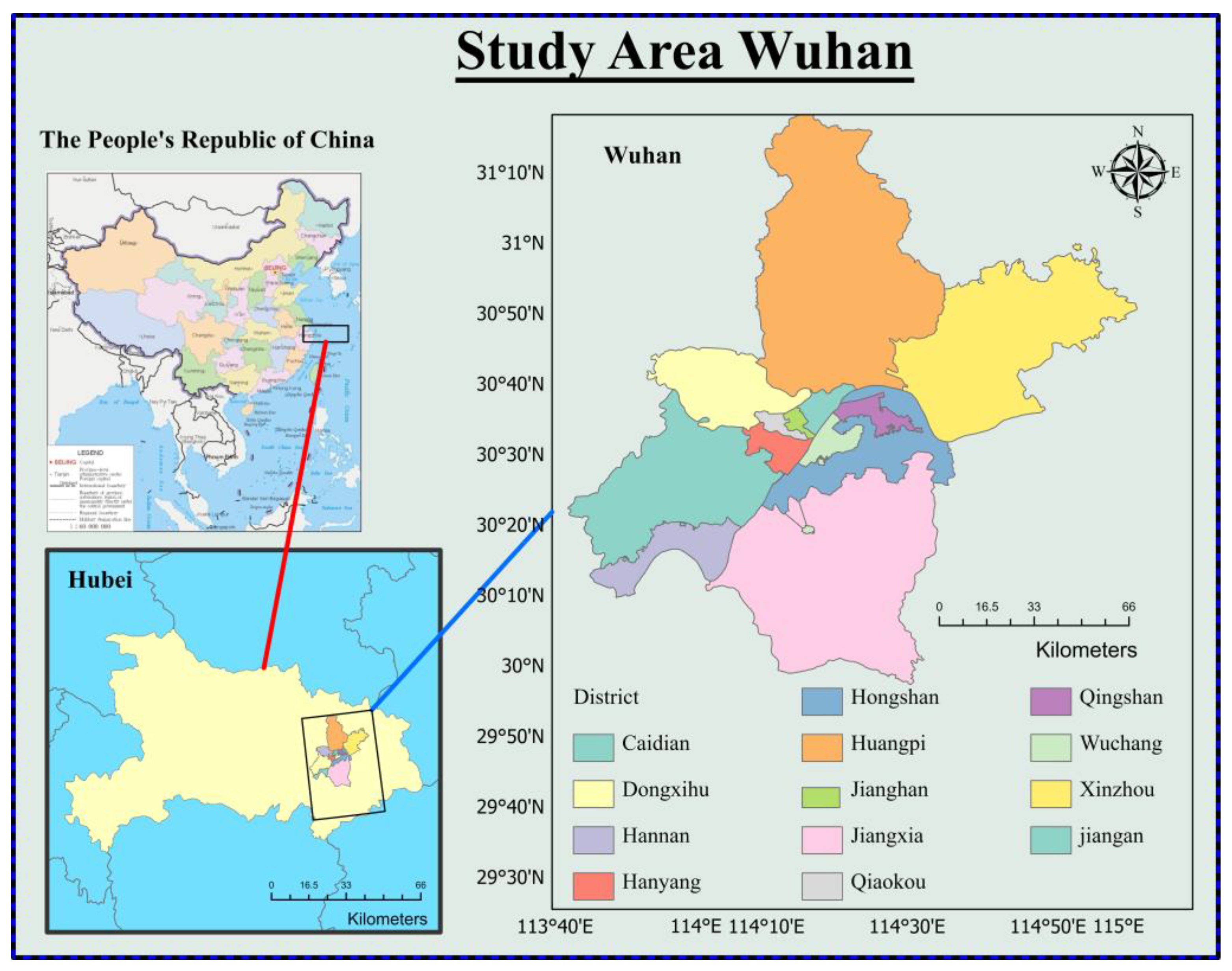
This approach combines a DNN model for estimating solar irradiance with atmospheric, geographical, and remote sensing data. High spatial resolution estimates of GHI and DNI are made using Sentinel-2 spectral bands and clear-sky indices from the Ineichen-Perez model, and they are verified against hyperspectral and ground-based irradiance data. The study space is where it starts. It begins with the study area, Wuhan, the capital of Hubei Province, which is a major urban center with over 11 million people and an area of 8494 km, as shown in Figure A1, and datasets describing the geographic context and satellite/ground observations. National and local policies, including carbon neutrality goals and incentives for renewable energy, highlight the need for accurate solar irradiance estimates to support sustainable development in Wuhan [32].

2.1. Atmospheric and Geospatial Data Acquisition

Ground-based and satellite-based data sources provide precise and validated solar irradiance modeling (see Table A2 and Table A3). The ability of each dataset to offer complementary information at different spatial and temporal resolutions is the basis for its selection. These datasets, which are processed and examined using Google Earth Engine (GEE), include crucial details on vegetation cover, surface reflectance, and atmospheric conditions, all of which have a major impact on solar irradiance. First, temporal alignment was accomplished by filtering each dataset to span the same time period in order to guarantee consistency across all datasets. Using filterDate (startDate, endDate), the ERA5 dataset, which offers global atmospheric data at an hourly temporal resolution, was filtered to fit the time span of the Sentinel-2 and Sentinel-5P datasets. This indicates that every data source reflects the same time period, enabling efficient integration. Sentinel-2 provides high-quality data at a resolution of 10 m, while ERA5 offers a resolution of 31 km. The reproject function in GEE was used to resample ERA5 to 10 m in order to correct the difference. Accurate fusion for model training is made possible by this resampling, which provides that all datasets have the same spatial resolution. Likewise, the 3.5 km spatial resolution of the Sentinel-5P Aerosol Index was resampled to 10 m.
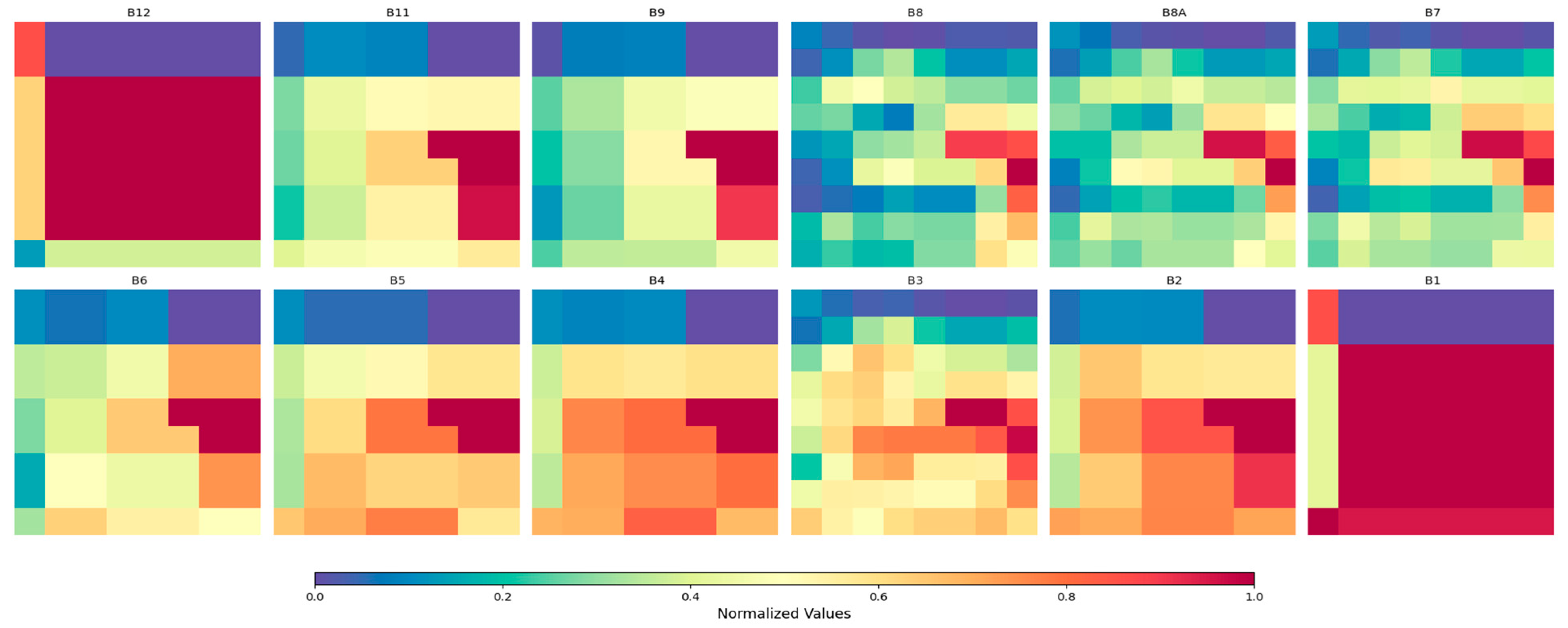
The datasets were combined to produce a complete input for deep learning models once they had been temporally and spatially matched. Sentinel-2 provided high-resolution surface reflectance data, ERA5 gave global atmospheric data, and the Sentinel-5P Aerosol Index provided information on aerosol concentrations. Furthermore, the combination of these datasets allows for an integrated method of predicting solar irradiance that concurrently takes atmospheric and surface parameters into account, increasing the accuracy of the model. The process of monthly Sentinel-2 imagery collection is where images are composited using a compositing function to create monthly composite images, as illustrated in Figure 1. It is especially difficult to integrate data from various sources in urban settings, such as high-resolution satellite imagery, ground-based atmospheric measurements, and real-time atmospheric features (such as cloud cover and aerosol concentration). Aligning datasets from many sources on the same day to produce a reliable and consistent input for the hybrid model is one of the main challenges. The hybrid model uses techniques that guarantee consistency and accuracy in the input data in order to overcome this. Additionally, the model improves training stability and overall model performance by identifying and prioritizing the most pertinent features using attention mechanisms and spectral band selection algorithms.
The primary source of data is Sentinel-2 multispectral imagery, which provides high-resolution measurements essential for estimating urban solar irradiance and covers the visible, near-infrared, and shortwave infrared bands. Sentinel-2 images are processed to exclude areas affected by cloud cover, ensuring that only valid clear-sky data is used. For the matching process, cloud-free satellite data on the same date is prioritized. These become merged into a single composite for each month, using a special compositing function. Once the monthly images from January to December have been compiled, a grid sampling method is used to select a set of sample points. The resulting data points are stored in a spatial database for DNN modeling. Additional data on GHI, DNI, air temperature, cloud cover, and aerosol concentrations, along with atmospheric factors such as height, aerosol index, solar zenith, and azimuth angles, are sourced from ground monitoring stations, the NSRDB, and model validation, enhancing accuracy. Furthermore, the solar irradiance model is validated using Environmental Mapping and Analysis Program (ENMAP) hyperspectral-derived irradiance estimates, which incorporate albedo, Normalized Difference Vegetation Index (NDVI) [33], and DSM data to account for surface reflectance characteristics and topographic variations affecting solar irradiance levels, as shown in Figure 2. Urban solar irradiance is influenced by both spatial and temporal variability, including factors like surface properties and atmospheric conditions.

2.2. Hybrid Modeling of Urban Solar Irradiance

The area hybrid model combines traditional atmospheric and geospatial data processing procedures along with advanced deep learning techniques for improving solar irradiance estimates [34].The model provides more accurate forecasts in a variety of metropolitan settings by integrating data from clear-, cloudy-, and all-sky situations. The hybrid model also leverages attention mechanisms to focus on the most important atmospheric and surface features that impact solar irradiance. This method helps to capture relevant data for urban conditions more accurately, improving the performance of the DNN in predicting solar irradiance in cities. The DNN component of the hybrid model is designed to learn from real-world data, adapting to urban-specific complexities like varying surface properties reflectance and absorption, enabling more accurate predictions of solar irradiance than traditional models [35]. In particular, utilizing Sentinel-2 imagery, it explores atmosphere, aerosol concentrations, and solar radiation measurements to evaluate environmental factors [36]. The deep learning model is trained using this satellite data to enable solar irradiance predictions, thus allowing accurate solar energy potential estimation across Wuhan. Furthermore, solar irradiance predictions are fundamental for solar energy potential assessment, particularly in light of the remote sensing and satellite data evaluation [37,38]. This section outlines the approaches, algorithms, and processes involved in irradiance assessment from differing sources. The complete workflow for this assessment is shown in Figure 3.

2.3. Preprocessing

Satellite-provided temperature, and T-ground, or ground station temperature, are aligned by Equation (A1). The datasets gathered from multiple sources during varying time periods were synchronized (see Table A2). It ensures that the time indicators of the ground data and satellites tally so that they can be effectively processed and validated. It was deemed useful to avoid incorporating solar zenith angles over about 85°, particularly during midday periods, because of distortions created by angular considerations. Hence, solar irradiances from Equation (A2) are more reliable, with data values normalized using Min-Max scaling. The model was improved through integrating atmospheric variables of temperature, AOD, and cloud probability, as these impact surface irradiances described in Equation (A3). The respective features deduced from the 12 bands of Sentinel-2 imaging were determined by Pearson correlation analysis on bands B3, B4, B8, B2, B8A, B11, and B12 at a correlation threshold of 0.95 (see Figure A3). This threshold ensures that the selected bands exhibit a strong linear relationship with the target variables, indicating that the bands are sufficiently correlated with the atmospheric and surface characteristics necessary for accurate solar irradiance prediction. A threshold below 0.95 could introduce more variability and noise into the model, while a higher threshold might exclude important but slightly less correlated bands. The benefits of this selection were the reduced dimensionality of data for the improved efficiency of computational processing required and of the accuracy of the DNN in estimating USIs over Wuhan [39,40,41,42]. The correlation between the two variables X and Y can be determined using the coefficient represented as given in Equation (1).
r ( X ,   Y ) = Cov ( X , Y ) σ X σ Y
To ensure optimal performance, a sensitivity analysis was conducted to fine-tune the hyperparameters of the DNN. Key hyperparameters such as learning rate, batch size, and number of layers were adjusted and tested for their impact on model performance. The sensitivity analysis allowed the identification of the most effective configuration, ensuring that the model could learn from the varied and complex urban data without overfitting. This step is critical for ensuring that the model can generalize well to unseen urban conditions, particularly in scenarios with cloud-affected data.

2.4. Clear-Sky Index Estimation

The CSI is determined as the ratio of the recorded irradiance to the clear-sky estimated irradiance obtained from the Perez–Ineichen model implemented in the PVLIB [6]. This means that the irradiance recorded is normalized against the optimum conditions of clear skies (as possible conditions) and includes atmospheric attenuation due to factors such as cloud and aerosol influence. Thus, the data is conditioned for input to the DNN, which can devote itself to real-world atmospheric conditions. In Equation (2), the measured irradiance of I_measured is due to ground-based measurements, while the clear-sky irradiance of I_clear-sky is the theoretical maximum due to conditions of clear-sky and no clouds. Normalizing I_measured by I_clear-sky tempers atmospheric variability, thus improving the model’s expenditure and predictive power. The GHI and DNI datasets are processed by quality procedures of noise filtering, gap filling, and consistency checking so that reliable data recording, the daily temporal resolution (day of month; DOM), and highly spatially resolved data of (10 × 10 m) are produced.
Such advanced datasets are vital for good solar irradiance modeling for providing suitable data to train the DNN. The clear-sky model is employed to give an estimate of the theoretical maximum irradiance and serves as a background for comparison against actual readings in the model, and gives the model realistic estimations of atmospheric influences. This establishes the reliability of the training process and gives improved predictive capacities. Cloud classification is taken using the Sentinel-2 scene classifier (SCL) [43], which gives the different types of clouds (clear, cloudy, cirrus). The reduced region shall compute the mean SCL value over a mean resolution of 30 m, which shall refine the input of the model. The SCL gives integer values to the different land and atmospheric phenomena, e.g., clear skies (SCL = 4), clouds (SCL = 8), cirrus clouds (SCL = 9). An accurate estimation of the CSI, through the deep learning medium, is a worthy goal in the enhancement of USI modeling and improving the reliability of solar resource assessment [37]. The CSI serves to normalize the irradiance values regenerated relative to their theoretical clear-sky condition. The spectral bands of Sentinel-2 are used as the input to the dense deep learning model with attention and skip layers, which add to the extraction of the feature values. The model output is the CSI values of the irradiance, which would have met the conditions of having high spatial-temporal resolution to provide the high spatial resolution required for suitable urban-scale solar resource assessment.
IneichenPerez CI = I _ measured I _ clear sky

2.5. Deep Neural Network-Based Solar Irradiance Estimation

Sentinel-2 satellite data enable accurate solar energy potential estimations [19,44]. Air temperature varied from 18.2 °C in Hannan and Caidian to 28.3 °C in Hongshan. Cloud probabilities ranged from 4% in Jianghan to 100% in Caidian, thus showing very variable atmospheric conditions (see Table A3). Figure 4 visualization of Sentinel-2 spectral input data used for CSI estimation, including both the seven selected spectral bands and the complete set of available bands. The color patterns represent normalized spectral intensity variations, where warmer colors indicate higher normalized values and cooler colors indicate lower normalized values within each band. Colors are used solely to illustrate spatial and spectral patterns and do not represent absolute physical reflectance or radiance values.The proposed hybrid model uses deep learning that can capture complex, non-linear relationships from high-resolution datasets so that better prediction results can be made regarding urban environments having variable local conditions [45]. The model also uses the Sentinel-2 spectral data that provide high-resolution spatial information in great detail, allowing more accurate estimates of solar energy potential. The DNN predicts the solar irradiance by learning the complex relationships between the input features, including Sentinel-2 spectral bands, atmospheric variables, and output irradiance [46,47,48]. The model consists of dense layers, attention mechanisms, and skip connections [49].
The Perez–Ineichen model provides a foundation for predicting clear-sky solar irradiance based on physical principles, using atmospheric parameters like solar zenith angle, air mass, and clear-sky conditions. However, the DNN does not simply use the output of the Perez–Ineichen model as an input. Instead, the DNN learns corrections to the theoretical predictions by incorporating real-world data such as cloud cover, aerosol concentration, and urban surface reflectance. These factors, which are not accounted for in the Perez–Ineichen model, introduce the need for the DNN to adapt and refine the predictions. The fusion mechanism between the Perez–Ineichen model and the DNN occurs through a data-driven learning process. To clarify the mathematical description of the fusion mechanism, the overall prediction of solar irradiance expressed in Equation (3):
I pred = I theory + f DNN ( X )
where I theory represents the irradiance predicted by the Perez–Ineichen model. f DNN ( X ) is represents the correction function learned by the DNN, which adjusts the theoretical prediction based on the input data X , including cloud cover, aerosol concentration, surface reflectance, and other atmospheric features. I pred is the final irradiance prediction made by the hybrid model.
Each of the spectral bands is processed through a dense layer, where the input is multiplied by a weight matrix and has a bias added to it, before applying a ReLU activation function to add non-linearity to the function, as shown in Equation (A4). By applying a consequence to large weights, L2 regularization is used in Equation (A5) to eliminate overfitting, limit the model’s complexity, and enhance generalization. Dropout of over 30% is used to eliminate overfitting, whilst Batch Normalization is introduced to stabilize the training regime and lessen the time until convergence, as expressed in Equation (A6). When making predictions or extracting features, the model can concentrate on the most pertinent portions of the data due to the attention ratings calculated by Equation (A7). The SoftMax Equation (A8) function is applied to normalize the weights applied to the attention mechanism. Additionally, skip connections are crucial because they improve the gradient’s flow, which raises convergence, and the back propagation may avoid a few layers. The output layer receives the concatenated feature vector and predicts the CSI value, or the ratio of the measured to clear-sky irradiance. According to Equation (4), the CSI is output, which is calculated as the ratio of the measured GHI/DNI to the clear-sky GHI/DNI values.
The data are divided into two sets: the first, the 7 key bands, and the second, all bands. Both sets are processed independently to train any model. In this case, they are modeling CSI with the input variable as the target. CSI values are used to indicate the possible solar energy potential. A total of 20% of the dataset is used for testing, and the remaining 80% is used for training. Following training, the model’s performance is assessed using the testing dataset. The DNI and GHI models’ training and validation loss curves for a single Wuhan site (see Figure A4). Further loss of models using all bands and using those of selected bands is observed, indicating the tackling of the model in the training model.
Clear   Sky   index   model = MGHI / DNI PCl   GHI / DNI
The supervised DNN model was trained using the Adam optimizer, which minimized the loss function. The lower the RMSE and MBE, the error in the evaluation of the accuracy of the predicted GHI, the greater the prediction accuracy. The RMSE, Equation (5), is computed based on the average of the squared difference between the actual GHI values (yi) and the estimated GHI (yn), which are then square rooted. Thus, we obtain some measure of the error that exists due to using estimations rather than actual values. The RMSE can also be expressed as the normalized RMSE (nRMSE), which represents the RMSE divided by the average of the actual GHI values (yo), with the result multiplied by 100 to express it in a percentage form in Equation (6). Thus, one can see the error in relationship to the actual values (sizes), giving some measure of the error relative to the size of the GHI. This is helpful when comparing one dataset to another. For this reason, Mean Bias Error (MBE), defined in Equation (7), was computed for the absolute differences in values between the GHI actual (yi) and the GHI estimated (yn), with the quantities of MBE being averaged. The normalized (nMBE) MBE in Equation (8) expresses MBE in the form of a percentage by dividing by the average of the actual GHI, DNI values (yo), and multiplying by 100. This presents an easier form of determining the magnitude of the prediction errors without squaring the absolute differences as in RMSE, thus the nMBE is not as sensitive when large prediction errors are experienced.
RMSE = 1 n i = 1 n y i yn 2
nRMSE = 1 1 n i = 1 n y i yn 2 yo × 100
MBE = 1 n i = 1 n | y i yn |
nMBE = 1 n i = 1 n | y i yn | yo × 100
The hyperparameters are used in the deep learning model for CSI estimation (see Table A4). These hyperparameters were selected to achieve optimal model performance. In order to avoid overfitting, the model employs dropout layers (0.4 to 0.2) and dense layers with ReLU activation that contain 256, 128, 64, and 32 neurons. StandardScaler for features and MinMaxScaler for the target are used to normalize the data after the model has been trained for 100 epochs with a batch size of 32. The hybrid model improves the precision and dependability of solar irradiance estimates by fusing deep learning methods with the PI model [50].

3. Results and Discussion

The results show that DNN-S delivers better results for GHI prediction, especially in districts where atmospheric variability and urban heterogeneity predominate, whereas DNN-A is better suited for DNI prediction, in which the USI component dominates. The opposite behavior of DNN-S and DNN-A demands that model inputs be adjusted to the irradiance component of interest, and demonstrates that the predictive effectiveness of deep learning systems for solar resource assessment is significantly impacted by the choice of spectral bands. Two DNN configurations with the same dense-layer architecture were compared to assess the impact of spectral band selection on model performance. The first was DNN-A, using all of the Sentinel-2 bands, and the second was DNN-S, using an input of seven bands chosen by correlation analysis. The architectures of the two models were identical in all respects, being formed of dense-layer networks with attention mechanisms, so that differences in performance can be attributed entirely to the input features and not the underlying structure.

3.1. Evaluation of Deep Neural Networks for Solar Irradiance Estimation

For GHI estimation, shown in Table 1, in most of the districts, the DNN-S model outperformed DNN-A, manifesting in lower RMSE values and bias. The DNN-S model in Hannan had a RMSE of 87 W/m2 (nRMSE = 34.6%), while the DNN-A model outperformed DNN-S by producing a RMSE of 122 W/m2 (nRMSE = 48.9%). In Qingshan, the DNN-S model produced the least amount of district-level errors (RMSE = 69 W/m2, nRMSE = 26.1%), indicating greater adaptability of the model in diffuse-radiation-dominated conditions. When averaged across all districts, DNN-S maintained a slight advantage, with an overall RMSE of 92.6 W/m2 versus 95.2 W/m2 for DNN-A, confirming that targeted band selection enhances model accuracy for global irradiance estimation. For DNI estimation, shown in Table 2, the best-performing result for DNI estimation was obtained by having an MBE of −7 W/m2 (nMBE = −1.6%) and a RMSE is 59 W/m2 (nRMSE = 12.8%), Hanyang under DNN-S, representing the most accurate and least biased prediction across all districts.

3.2. Comparing Performance in Clear-Sky and Cloudy Conditions

In order to ensure correct estimation of solar irradiance and assess stability under atmospheric fluctuation, it is crucial to evaluate the model’s performance under both clear- and overcast-sky situations. In clear-sky instances, DNN-S comes up with a RMSE of 89 W/m2 and MBE = 0.8; whereas DNN-A comes up with a RMSE equal to 95 W/m2 and MBE = −24.5 (see Table 3). These results indicate that DNN-S was more satisfactorily able to predict GHI also in clear-sky intervals than was the case with DNN-A. When comparing clear-sky models, the seven chosen bands, and all bands, GHI and DNI receive different results in terms of their estimates throughout the Wuhan districts. However, the estimates based on the seven bands are quite close to those based on all bands. Because it is feasible to obtain the growth of the seasonal and geographical irradiance, using too few bands reduces the interval in the calculation.
Under clear-sky conditions, DNN-S achieved a RMSE of 69 W/m2 (nRMSE = 10.54%) with an MBE of –12.3 W/m2, whereas DNN-A produced a substantially higher RMSE of 107 W/m2 and a stronger negative bias of –62.3 W/m2. This shows that DNN-S provides more accurate and less biased DNI predictions compared to DNN-A, as shown in Table 4.

3.3. Error Analysis

The characteristics of clouds and aerosols play a significant role in radiation absorption and transmission. Consequently, the accuracy of GHI estimates is checked using the spatial distributions of aerosol optical thickness, cloud optical thickness, and cloud type. As seen in Figure 5, the models were evaluated in clear-sky, cloudy-sky, and all-sky scenarios. Examining the residual differences between predicted and observed solar irradiance estimates, along with their correlation to important meteorological variables such as cloud cover and aerosol concentration, is part of the error attribution methodology.. The normalized nRMSE and nMBE for clear-, overcast-, and all-sky conditions across different Wuhan districts are shown in bar graphs. These charts illustrate the model performs differently under various atmospheric situations. While the all-sky nRMSE represents the model’s overall error across all scenarios, the clear-sky and cloudy-sky nRMSEs display the error across all weather circumstances. The bar graphs show that districts like Jiangxia and Qiaokou exhibit higher residual errors, particularly under cloudy-sky and all-sky conditions, indicating these areas are more affected by cloud cover and aerosol concentration.
The DNN-S models give rise to decreased GHI errors under clear-sky conditions. Districts such as Xinzhou and Huangpi show a decrease in nRMSE. The DNN-S model continues with the sequence of all bands for DNI, in foggy conditions, and provides proof of its usefulness. The DNN-S model demonstrate lower nMBE in the areas of Jianghan and Dongxihu, although the areas with compound cloud conditions show a high nRMSE in these areas. In most parts of the city, especially Wuchang and Jiangxia, the seven chosen bands provide good results in all sky circumstances, with a decreased error and bias in the GHI and DNI computations.

3.4. Solar Irradiance Estimation Using Sentinel-2 Imagery

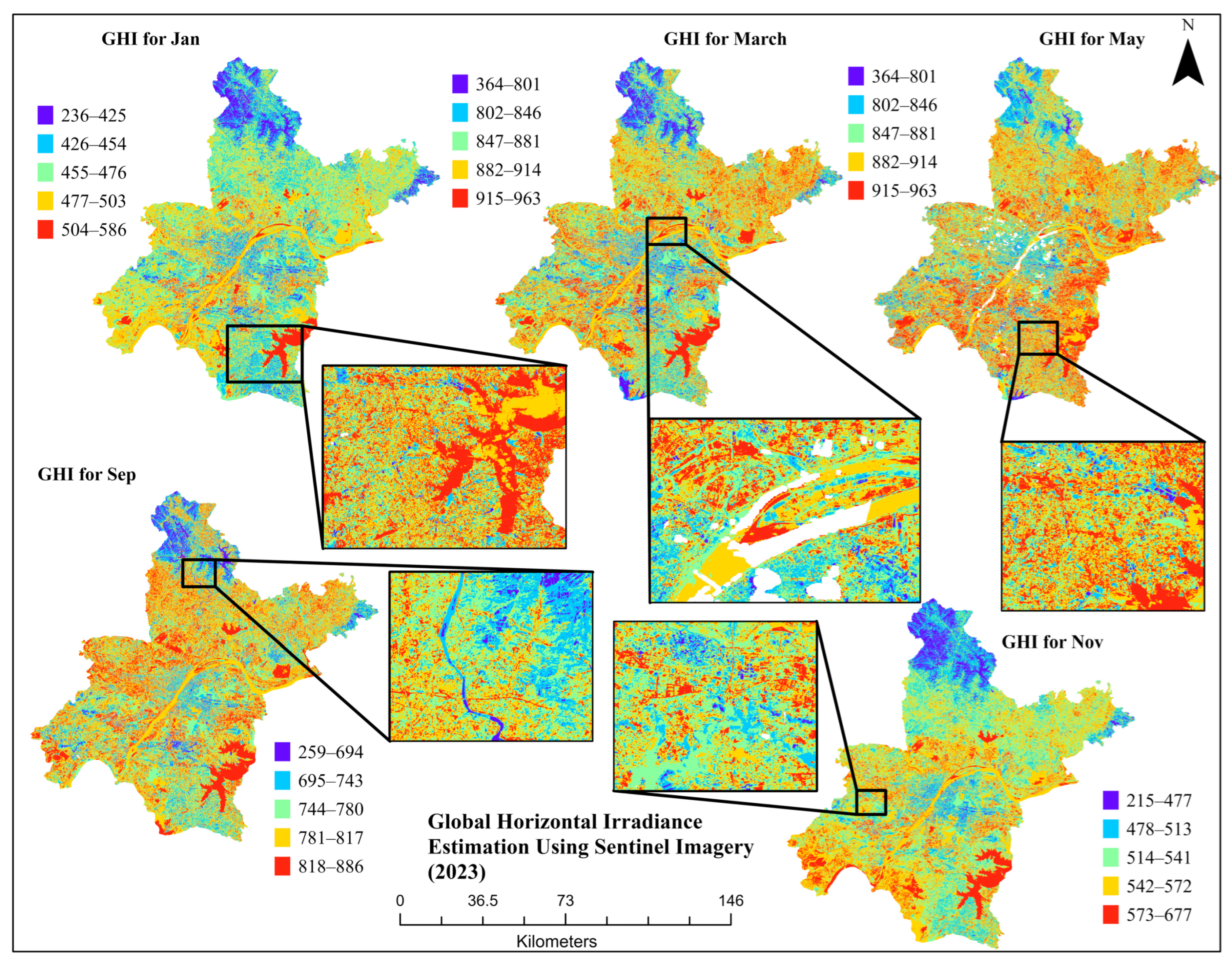
The DNN-S model computes the DNI spatial distribution for selected months of 2023, based on its seven spectral bands, for periods when the seasonal variation in irradiance is also evident in the profile. From Figure 6, because of low solar angles and overcast skies, January and December have low DNI values, whereas May and June have the highest values due to more sunshine hours and less air dispersion. The blue areas are characterized by low irradiance conditions, influenced by shading or something else due to air conditioning. The areas with red are influenced by a strong potential for installing solar power programs. The DNN-S model also calculates the GHI estimates for sections of Wuhan for the periods of January, March, May, September, and November of 2023, as shown in Figure 7.

3.5. Validation of GHI and DNI Estimates Using Hyperspectral Imagery

The aspect, slope, and angles of the sun for Wuhan have been determined using the geographic elements of latitude, elevation, and DSM to determine the amount of solar energy absorbed by the Earth’s surface. It makes use of hyperspectral images to increase the precision of GHI and DNI by taking the vegetation cover (NDVI) and reflectance of the surface (albedo) into account. With ENMAP’s hyperspectral images, the estimates of solar irradiation have been verified. This validation has the purpose of establishing the accuracy of the estimates of the DNI and GHI, and to improve the model with a wider field of action in urban environments. Figure 8 illustrates the comparison between the DNI estimates derived from Sentinel-2 and ENMAP hyperspectral data. Panel A shows the overall DNI distribution across Wuhan, highlighting varying irradiance levels. Panels B and C display ENMAP hyperspectral-based estimations of DNI, zooming into smaller areas for validation of the Senti-nel-2 irradiance estimates, providing detailed views of DNI patterns in those regions. Panel D further zooms into a high-resolution section, offering a closer comparison of the two datasets in an area with high irradiance values. Finally, E focuses on a region with low irradiance values, enabling a comparison of the quality and correlation of the data from both Sentinel-2 and ENMAP and 9. Figure 9 illustrates the comparison of Global Horizontal Irradiance (GHI) estimates derived from Sentinel-2 and ENMAP Hyperspectral data. Panel A shows the overall GHI distribution across Wuhan, high-lighting varying irradiance levels, with a color gradient indicating different GHI values. Panels B and C display ENMAP hyperspectral-based GHI estimations, zooming into smaller regions corresponding to areas in the Sentinel-2 map shown in Panel A. Panel B provides a broader view of the ENMAP data in a section of the region, while Panel C focuses on a smaller, high-resolution area within the same region. These panels are used for validating the GHI estimates from Sentinel-2 by comparing them to the corresponding ENMAP data. Panel D zooms into a high-resolution section, offering a closer comparison of the GHI values from both datasets in areas with higher irradiance. Finally, Panel E focuses on a region with lower irradiance values, allowing for a comparison of the quality and correlation of the GHI data from both Sentinel-2 and ENMAP. However, in areas with more complicated topography or varied vegetation, there were discrepancies in the estimates with respect to the hyperspectral data of ENMAP, which gave better resolution and accuracy in the DNI. According to these results, it can be said that Sentinel-2 is generally reliable for modeling solar irradiance in areas of little variability in land cover, but in more complex areas, these must be calibrated more accurately in order to improve their knowledge of solar energy applications across.
Combining Sentinel-2 spectral data with deep learning techniques has demonstrated significant effectiveness in accurately estimating solar irradiance within complex urban environments. The proposed framework overcomes the spatial and atmospheric limitations of traditional methods, leading to enhanced estimation accuracy. The study obtains strong USI predictions by using seven carefully chosen spectral bands, including B8A, B11, B2, B3, B4, B8, and B12, in conjunction with ground-truth measurements from the NSRDB and an advanced Deep Neural Network architecture with attention mechanisms and skip connections. These results highlight the advantages of combining deep learning with high-resolution satellite imagery for solar resource analysis, demonstrating the effectiveness of this approach in addressing challenges related to atmospheric variability and urban architecture when compared to previous studies that relied on GOES or MODIS data.

4. Discussion

Sentinel-2 imagery utilization in the proposed framework offers significant benefits over earlier research, particularly for applications at the urban scale. On the other hand, data from geostationary satellites with a temporal resolution of five minutes and a spatial resolution of roughly one kilometer was employed [3]. While their approach achieved lower RMSE values, the rough spatial resolution limits its capability to capture urban-specific features. In contrast, our study’s 10 m resolution enabled Sentinel-2 to capture detailed mapping of irradiance variations, critical for applications like rooftop solar planning. Compared to MODIS-based studies, such as [18], which used 1 km resolution data, our approach better resolves urban microclimates, as reflected by reduced RMSE and nMBE values in Huangpi and Xinzhou. DNN-S’s DNI RMSE of 87.60 W/m2 in cloudy skies, compared to DNN-A’s 124.33 W/m2, highlights the attention mechanism’s effectiveness. Additionally, unlike physical radiative transfer models [11], which require extensive computational resources and detailed atmospheric inputs [6], the deep learning model reduces computational complexity by forty percent through band selection.
A further comparison with current techniques based on machine learning shows this, such as [51]. However, it faced challenges in capturing fine-scale spatial variations within urban environments. The combination of deep learning with Sentinel-2 high-resolution imagery and ground measurements in our study offers a more robust solution, especially for complex atmospheric conditions in Wuhan, as evidenced by lower nMBE values in districts such as Hannan and Qiaokou.
The key strength of this study is its high-resolution approach, leveraging Sentinel-2’s 10 m spatial resolution to capture urban-specific irradiance variations, a factor often neglected in earlier studies that used lower-resolution data. This resolution is especially beneficial for urban energy planning and facilitating accurate assessments of solar potential in the diverse districts of Wuhan [52]. Another key strength is the use of attention mechanisms, which enable the model to dynamically prioritize critical features, such as cloud cover. This innovation reduced errors in cloudy conditions by up to 20% compared to DNN-A. The Pearson correlation analysis, selecting seven bands, reduced computational complexity by making the model scalable for large-scale applications.
The integration of ground measurements with Sentinel-2 imagery provided a robust dataset, enhancing model validation and reliability. The model’s performance across clear and cloudy skies demonstrates its adaptability to variable atmospheric conditions, a challenge for traditional models. Additionally, the framework’s implementation in TensorFlow and the use of regularization techniques ensured stable training and generalizability. The density is represented as a normalized probability distribution, with each distribution fitted using Gaussian regression to capture the spread and concentration of errors. Narrower distributions indicate that the predicted values are generally closer to the measured data, reflecting higher precision and lower variability. When comparing the performance of models using all spectral bands versus selected bands, the error distributions for the selected bands display a noticeably narrower profile. This suggests that careful selection of spectral bands enhances model accuracy and reduces estimation uncertainty for both GHI and DNI.
High-resolution information on surface reflectance, albedo, and NDVI is provided by ENMAP hyperspectral images and is essential for calculating GHI and DNI. It validates Sentinel-2 GHI estimations by taking vegetation impacts and reflection into account. By measuring the absorption or reflection of sunlight, albedo, and NDVI have an impact on solar irradiance. High albedo surfaces, like snow or cities, contrast with low albedo areas, like forests or water. Vegetation density, which influences solar energy absorption, is reflected in the NDVI. In order to provide correct energy modeling, DSM and area solar radiation maps take topography and surface reflectivity into account when validating solar radiation estimates.
This study enhances urban solar resource assessment by combining high-resolution Sentinel-2 imagery with deep learning, providing a more efficient and scalable approach to solar energy planning. The model’s integration with ground-level measurements ensures robust validation and better generalizability. The error analysis, using a normalized probability distribution fitted with Gaussian regression, shows that the selected bands result in a narrower error distribution, further enhancing accuracy and reducing uncertainty in USI prediction.

5. Conclusions

This research successfully develops a hybrid method based on the PI model combined with a DNN, which is used to predict the USI in Wuhan, China. Using the Sentinel-2 multispectral data together with real-time atmospheric data allows the inclusion of important atmospheric parameters (cloud cover, aerosol concentration, and surface reflectance). The use of a CSI and attention in the DNN model greatly increases the performance, allowing a better estimation of the solar irradiance in different sky conditions. Comparing the DNN-S (selected bands) and the DNN-A models, it is confirmed that the DNN-S model has a better overall accuracy, since it shows lower Root Mean Squared Errors (RMSE) in each sky condition. Since the estimations correspond extremely well with the actual irradiance, the verification with regard to the hyperspectral-based irradiance further demonstrates the model’s robustness. This work demonstrates the possibility of combining deep learning with satellite-based information for urban solar irradiance estimations, giving a scalable and robust product, which is an important tool for planners in the solar energy sector in different urban zones. Although this framework seems strong in Wuhan, it would, in future research, be interesting to consider cases in other urban zones, the development of more refined feature selections, and, finally, also including other temporal and spatial data, which would contribute to a more accurate and versatile model. It should also be able to support a more informed way of using and giving political support for the implementation of the infrastructure for different renewable energy solutions, by seeking to raise more sustainable urban energy solutions.

Author Contributions

Conceptualization, Z.K.H., C.J. and R.W.A.; methodology, Z.K.H. and R.W.A.; investigation, Z.K.H., C.J. and R.W.A.; writing—original draft, Z.K.H., C.J. and R.W.A.; writing—review and editing, Z.K.H., C.J. and R.W.A.; funding acquisition, C.J.; resources, C.J.; supervision, C.J. All authors have read and agreed to the published version of the manuscript.

Funding

This work is supported by the National Key Research and development plan: Research on global remote sensing inventory methods of greenhouse gases (No. 2021YFE0118000); Research on point source CO2 emission satellite remote sensing monitoring method based on imaging spectrometer by the National Natural Science Foundation of China (No. 42475144).

Data Availability Statement

The data used in this research is publicly available and can be accessed via the following link (accessed on 10 March 2025): https://github.com/uzeenat/Satellite-Project.git. The dataset includes monthly solar radiation data, land use data, and other environmental data specific to Wuhan. These data sources are essential for conducting remote sensing analysis and deep learning model evaluation.

Conflicts of Interest

The authors declare that they have no conflicts of interest related to the content of this manuscript. There are no financial, professional, or personal relationships that could influence the research or interpretation of results.

Appendix A

Figure A1. Geographic representation of Wuhan with administrative districts.
Remotesensing 18 00033 g0a1
Figure A2. Sentinel-2 image of Wuhan on 10 January 2023 (20:45 UTC), showing all 13 spectral bands.
Remotesensing 18 00033 g0a2
Figure A3. Sentinel-2 spectral features: an inter-band correlation analysis for GHI and DNI prediction.
Remotesensing 18 00033 g0a3
Figure A4. The loss curves for training and validation of the DNI and GHI models: (A) DNI loss with all bands, (B) DNI loss with selected bands, (C) GHI loss with all bands, (D) GHI loss with selected bands, estimates at a single Wuhan location.
Remotesensing 18 00033 g0a4
Figure A5. The error distributions for GHI and DNI estimates across all Wuhan districts.
Remotesensing 18 00033 g0a5
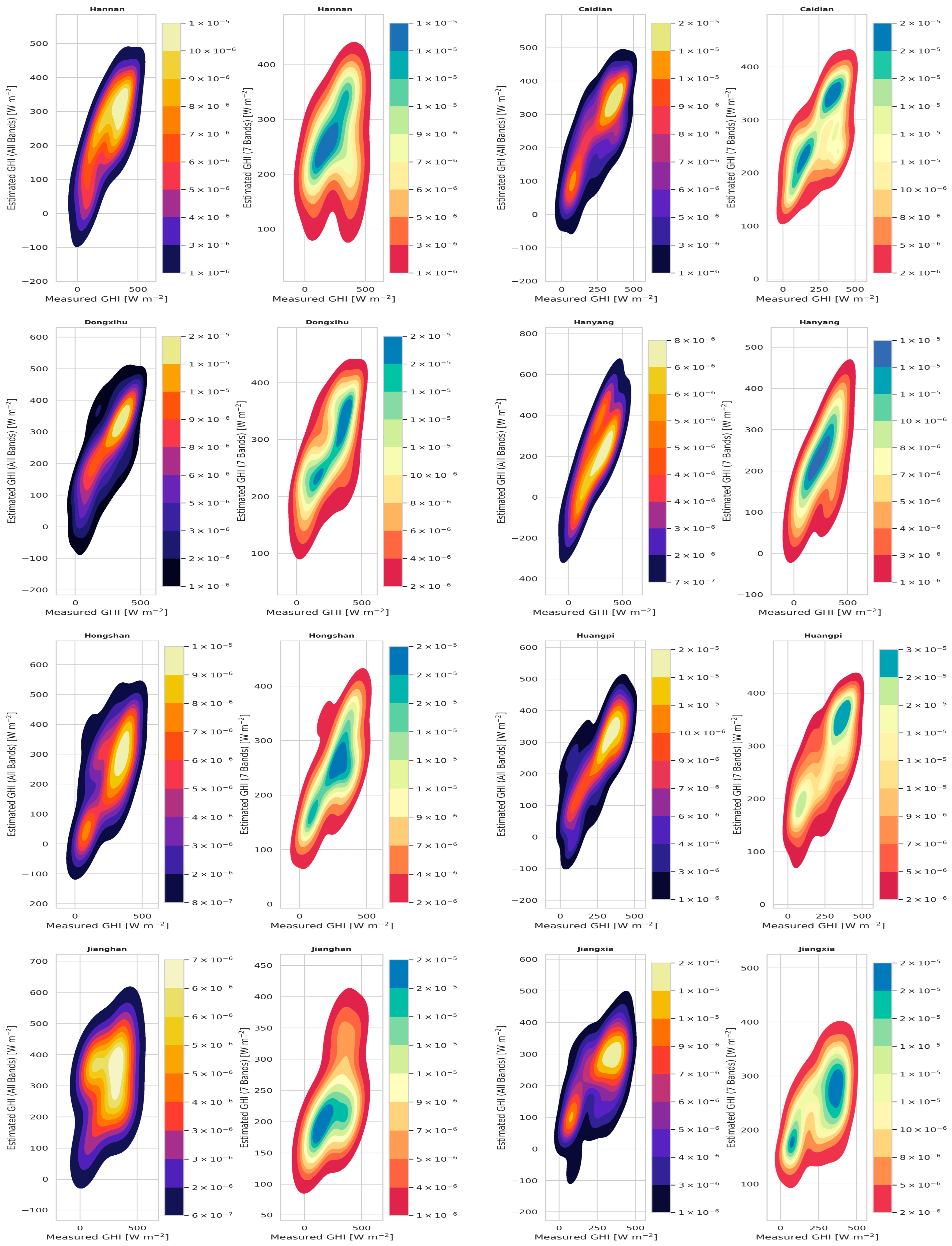
Figure A6. Density scatter plots comparing measured GHI with the GHI estimated using all bands and selected bands across various districts in Wuhan. Each district’s data is represented in a grid format.
Remotesensing 18 00033 g0a6
Figure A7. Density scatter plots comparing measured DNI with the DNI estimated using all bands and selected bands across various districts in Wuhan. Each district’s data is represented in a grid format.
Remotesensing 18 00033 g0a7
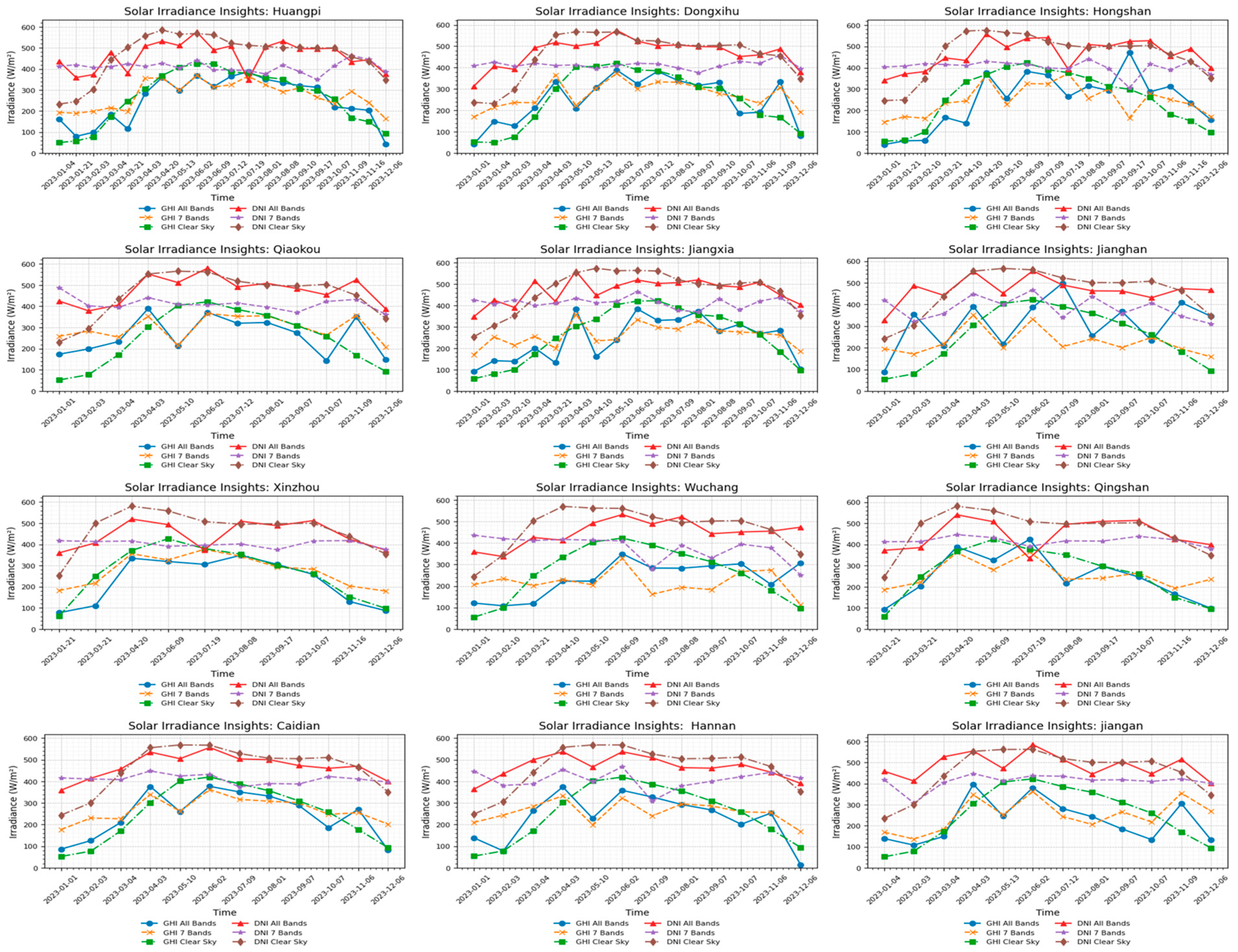
Figure A8. Temporal variations in GHI and DNI across Wuhan’s districts using all spectral bands, seven selected bands, and clear-sky estimates.
Remotesensing 18 00033 g0a8
Table A1. Comparison of Sentinel-2 and ENMAP datasets for solar irradiance.
DatasetTypeCoverageTemporal FrequencyUsage
Sentinel-2MultispectralLarge
(100+ km2)
Every 5 daysMain dataset for GHI/DNI modeling
EnMAPHyperspectralSmall
(30 km width)
Single dateHigh-quality reference (validation)
Table A2. Datasets and parameters for atmospheric and solar analysis.
ParameterAccess Date Dataset
NDVI, Solar Geometry, AlbedoAccessed on 18 June 2024https://www.enmap.org/
Aerosol IndexAccessed on 18 June 2024Sentinel-5P NRTI L3 Aerosol Index (COPERNICUS/S5P/NRTI/L3_AER_AI)
Solar AzimuthAccessed on 18 June 2024Sentinel-5P NRTI L3 Aerosol Index (COPERNICUS/S5P/NRTI/L3_AER_AI)
Solar Zenith AngleAccessed on 18 June 2024Sentinel-5P NRTI L3 Aerosol Index (COPERNICUS/S5P/NRTI/L3_AER_AI)
Air TemperatureAccessed on 18 June 2024ERA5 Daily Aggregates (ECMWF/ERA5/DAY)
Cloud MaskAccessed on 18 June 2024Sentinel-2 Surface Reflectance (COPERNICUS/S2_SR)
Clear Sky IndexAccessed on 18 June 2024Sentinel-2 Surface Reflectance (COPERNICUS/S2_SR)
Atmospheric dataAccessed on 18 June 2024https://nsrdb.nrel.gov
All spectral bandsAccessed on 18 June 2024COPERNICUS/S2_SR_HARMONIZED
Altitude (Elevation)Accessed on 18 June 2024SRTM Digital Elevation Model (USGS/SRTMGL1_003)
Table A3. Ground-level meteorological and environmental measurements for Wuhan’s 13 districts.
DistrictAir Temperature (°C)Altitude (m)Latitude
DD:DD
Longitude
DD:DD
Cloud Probability %
Hannan18.22530.28114.0147
Caidian18.21730.64113.9310
Dongxihu18.32130.64114.1140
Hanyang18.32330.56114.1921
Hongshan28.31530.64114.555
Huangpi27.61830.82114.475
Jianghan18.31630.60114.274
Jiangxia26.51630.20114.474
Qiaokou18.31730.58114.2117
Qingshan28.42230.64114.378
Wuchang26.22030.56114.378
Xinzhou28.31630.74114.736
Jiangan8.31930.64114.2926
Table A4. Hyperparameter settings of the DNN–S model for GHI and DNI estimation using Sentinel-2 data.
HyperparameterValue
All BandsStandard Scaler
Selected BandsStandard Scaler
GHI and DNIMin-Max Scaler
Test Size0.2
Random State42.0
Dense Layer 1 (input all bands; input selected bands) 256 neurons, activation = ReLU
Dropout 1 (input all bands; input selected bands) 0.4
Dense Layer 2 (input all bands; input selected bands) 128 neurons, activation = ReLU
Dropout 2 (input all bands; input selected bands) 0.3
Dense Layer 3 (input all bands; input selected bands) 128 neurons, activation = ReLU
Dropout 3 (input all bands; input selected bands)0.3
Dense Layer 4 (input all bands; input selected bands) 64 neurons, activation = ReLU
Dropout 4 (input all bands; input selected bands)0.2
Dense Layer 5 (input all bands; input selected bands) 32 neurons, activation = ReLU
Output Layer1 neuron, activation = linear
OptimizerAdam
Loss FunctionMSE
MetricsMAE
Epochs100.0
Batch Size32.0
Aligned = min ( T _ satellite ,   T _ ground )
where T_satellite is the temperature derived from data collected by satellite remote sensing. The base T_ground is the temperature that ground stations directly measure.
X _ norm =   ( X X _ min )     ( X _ max X _ min )
I =   I 0 · e AOD · k
In this equation, the original data value is represented by X, the minimum value in the dataset is denoted as X_min, and the maximum value in the dataset is denoted as X_max. The normalized value, X_norm, is scaled between 0 and 1, ensuring all data points are within a uniform range. The Sentinel-2 bands were normalized according to Min-Max scaling onto a common range from 0 to 1 so that they contributed equally during the model-training phase.
Output i = ReLU ( W i · X i + b i )
where Xi is the input corresponding to each of the spectral bands i, Wi is the weights attached to each of the i-th spectral band, and bi is the bias part corresponding to the i-th band.
Loss L 2 = λ i = 1 n w i 2
where wi are the weights of the model and λ is the regularization term. Normal initialization is used to eliminate problems with vanishing gradients.
X = x μ σ
where μ is the mean and σ is the standard deviation of the sample.
Attention   Output i = Softmax ( Q i · K i ) V i
Qi is the query vector corresponding to the i-th band, Ki is the key vector data attached to the i-th band, and Vi are the value vector elements attached to the i-th band.
Softmax x i = e x i j e xij
Xi is the SoftMax function, and e x i t is the exponential function to the input. j e x i j is the sum of exponentials of all the inputs.

References

  1. Kim, J.; Kim, E.; Jung, S.; Kim, M.; Kim, B.; Kim, S. Improved Surface Solar Irradiation Estimation Using Satellite Data and Feature Engineering. Remote Sens. 2025, 17, 65. [Google Scholar] [CrossRef]
  2. Bright, J.M.; Sun, X.; Gueymard, C.A.; Acord, B.; Wang, P.; Engerer, N.A. BRIGHT-SUN: A Globally Applicable 1-Min Irradiance Clear-Sky Detection Model. Renew. Sustain. Energy Rev. 2020, 121, 109706. [Google Scholar] [CrossRef]
  3. Chen, S.; Li, C.; Xie, Y.; Li, M. Global and Direct Solar Irradiance Estimation Using Deep Learning and Selected Spectral Satellite Images. Appl. Energy 2023, 352, 121979. [Google Scholar] [CrossRef]
  4. Liu, F.; Wang, X.; Sun, F.; Wang, H. Correct and Remap Solar Radiation and Photovoltaic Power in China Based on Machine Learning Models. Appl. Energy 2022, 312, 118775. [Google Scholar] [CrossRef]
  5. Okada, J.; Ai, B.; Tomoyama, G.; Sakurai, N.; Fujiwara, Y.; Hoshi, T. The Structure of Health Factors among Community-dwelling Elderly People. City Res. 2003, 81, 19–30. [Google Scholar]
  6. Mendyl, A.; Mabasa, B.; Bouzghiba, H.; Weidinger, T. Calibration and Validation of Global Horizontal Irradiance Clear Sky Models against McClear Clear Sky Model in Morocco. Appl. Sci. 2023, 13, 320. [Google Scholar] [CrossRef]
  7. Thornton, P.E.; Hasenauer, H.; White, M.A. Simultaneous Estimation of Daily Solar Radiation and Humidity from Observed Temperature and Precipitation: An Application over Complex Terrain in Austria. Agric. For. Meteorol. 2000, 104, 255–271. [Google Scholar] [CrossRef]
  8. Barancsuk, L.; Groma, V.; Günter, D.; Osán, J.; Hartmann, B. Estimation of Solar Irradiance Using a Neural Network Based on the Combination of Sky Camera Images and Meteorological Data. Energies 2024, 17, 438. [Google Scholar] [CrossRef]
  9. Tapakis, R.; Charalambides, A.G. Enhanced Values of Global Irradiance Due to the Presence of Clouds in Eastern Mediterranean. Renew. Energy 2014, 62, 459–467. [Google Scholar] [CrossRef]
  10. Laguarda, A.; Giacosa, G.; Alonso-Suárez, R.; Abal, G. Performance of the Site-Adapted CAMS Database and Locally Adjusted Cloud Index Models for Estimating Global Solar Horizontal Irradiation over the Pampa Húmeda. Sol. Energy 2020, 199, 295–307. [Google Scholar] [CrossRef]
  11. Qu, Z.; Oumbe, A.; Blanc, P.; Espinar, B.; Gesell, G.; Gschwind, B.; Klüser, L.; Lefèvre, M.; Saboret, L.; Schroedter-Homscheidt, M.; et al. Fast Radiative Transfer Parameterisation for Assessing the Surface Solar Irradiance: The Heliosat-4 Method. Meteorol. Z. 2017, 26, 33–57. [Google Scholar] [CrossRef]
  12. Lefèvre, M.; Oumbe, A.; Blanc, P.; Espinar, B.; Gschwind, B.; Qu, Z.; Wald, L.; Schroedter-Homscheidt, M.; Hoyer-Klick, C.; Arola, A.; et al. McClear: A New Model Estimating Downwelling Solar Radiation at Ground Level in Clear-Sky Conditions. Atmos. Meas. Tech. 2013, 6, 2403–2418. [Google Scholar] [CrossRef]
  13. Chen, S.; Li, M. Improved Turbidity Estimation from Local Meteorological Data for Solar Resourcing and Forecasting Applications. Renew. Energy 2022, 189, 259–272. [Google Scholar] [CrossRef]
  14. Yi, Y.; Zheng, Z.; Lv, T.; Dong, J.; Yang, J.; Lin, Z.; Li, S. Nowcasting of Surface Solar Irradiance Based on Cloud Optical Thickness from GOES-16. Remote Sens. 2025, 17, 2861. [Google Scholar] [CrossRef]
  15. Mueller, R.W.; Dagestad, K.F.; Ineichen, P.; Schroedter-Homscheidt, M.; Cros, S.; Dumortier, D.; Kuhlemann, R.; Olseth, J.A.; Piernavieja, G.; Reise, C.; et al. Rethinking Satellite-Based Solar Irradiance Modelling: The SOLIS Clear-Sky Module. Remote Sens. Environ. 2004, 91, 160–174. [Google Scholar] [CrossRef]
  16. Chen, J.; Zhu, W.; Yu, Q. Estimating Half-Hourly Solar Radiation over the Continental United States Using GOES-16 Data with Iterative Random Forest. Renew. Energy 2021, 178, 916–929. [Google Scholar] [CrossRef]
  17. Schmit, T.J.; Lindstrom, S.S.; Gerth, J.J.; Gunshor, M.M. Applications of the 16 Spectral Bands on the Advanced Baseline Imager (ABI). J. Oper. Meteorol. 2018, 06, 33–46. [Google Scholar] [CrossRef]
  18. Zhang, Y.; Ren, J.; Pu, Y.; Wang, P. Solar Energy Potential Assessment: A Framework to Integrate Geographic, Technological, and Economic Indices for a Potential Analysis. Renew. Energy 2020, 149, 577–586. [Google Scholar] [CrossRef]
  19. Zhang, P.; Weng, J.; Kang, Q.; Li, J. Reconstruction of High-Resolution Solar Spectral Irradiance Based on Residual Channel Attention Networks. Remote Sens. 2024, 16, 4698. [Google Scholar] [CrossRef]
  20. Ajith, M.; Martínez-Ramón, M. Deep Learning Based Solar Radiation Micro Forecast by Fusion of Infrared Cloud Images and Radiation Data. Appl. Energy 2021, 294, 117014. [Google Scholar] [CrossRef]
  21. Salazar, G.; Gueymard, C.; Galdino, J.B.; de Castro Vilela, O.; Fraidenraich, N. Solar Irradiance Time Series Derived from High-Quality Measurements, Satellite-Based Models, and Reanalyses at a near-Equatorial Site in Brazil. Renew. Sustain. Energy Rev. 2020, 117, 109478. [Google Scholar] [CrossRef]
  22. Chen, J.; Zhu, W.; Yu, Q. High-Spatiotemporal-Resolution Estimation of Solar Energy Component in the United States Using a New Satellite-Based Model. J. Environ. Manag. 2022, 302, 114077. [Google Scholar] [CrossRef]
  23. Mikofski, M.M.; Hansen, C.W.; Holmgren, W.F.; Kimball, G.M. Use of Measured Aerosol Optical Depth and Precipitable Water to Model Clear Sky Irradiance. In Proceedings of the 2017 IEEE 44th Photovoltaic Specialist Conference (PVSC 2017), Washington, DC, USA, 25–30 June 2017; pp. 110–116. [Google Scholar] [CrossRef]
  24. Chen, S.; Liang, Z.; Guo, S.; Li, M. Estimation of High-Resolution Solar Irradiance Data Using Optimized Semi-Empirical Satellite Method and GOES-16 Imagery. Sol. Energy 2022, 241, 404–415. [Google Scholar] [CrossRef]
  25. Yang, D.; Wang, W.; Gueymard, C.A.; Hong, T.; Kleissl, J.; Huang, J.; Perez, M.J.; Perez, R.; Bright, J.M.; Xia, X.; et al. A Review of Solar Forecasting, Its Dependence on Atmospheric Sciences and Implications for Grid Integration: Towards Carbon Neutrality. Renew. Sustain. Energy Rev. 2022, 161, 112348. [Google Scholar] [CrossRef]
  26. Karalasingham, S.; Deo, R.C.; Raj, N.; Casillas-Perez, D.; Salcedo-Sanz, S. Generating High Spatial and Temporal Surface Albedo with Multispectral-Wavemix and Temporal-Shift Heatmaps. Remote Sens. 2025, 17, 461. [Google Scholar] [CrossRef]
  27. Yagli, G.M.; Yang, D.; Gandhi, O.; Srinivasan, D. Can We Justify Producing Univariate Machine-Learning Forecasts with Satellite-Derived Solar Irradiance? Appl. Energy 2020, 259, 114122. [Google Scholar] [CrossRef]
  28. Chu, Y.; Li, M.; Coimbra, C.F.M. Sun-Tracking Imaging System for Intra-Hour DNI Forecasts. Renew. Energy 2016, 96, 792–799. [Google Scholar] [CrossRef]
  29. Sooriyaarachchi, V.; Wijeratne, L.O.H.; Waczak, J.; Patra, R.; Lary, D.J.; Zhang, Y. Enhancing Hyperlocal Wavelength-Resolved Solar Irradiance Estimation Using Remote Sensing and Machine Learning. Remote Sens. 2025, 17, 2753. [Google Scholar] [CrossRef]
  30. Aslam, R.W.; Shu, H.; Tariq, A.; Naz, I.; Ahmad, M.N.; Quddoos, A.; Javid, K.; Mustafa, F.; Aeman, H. Monitoring Landuse Change in Uchhali and Khabeki Wetland Lakes, Pakistan Using Remote Sensing Data. Gondwana Res. 2024, 129, 252–267. [Google Scholar] [CrossRef]
  31. Kabir, E.; Kumar, P.; Kumar, S.; Adelodun, A.A.; Kim, K.H. Solar Energy: Potential and Future Prospects. Renew. Sustain. Energy Rev. 2018, 82, 894–900. [Google Scholar] [CrossRef]
  32. Li, M.; Virguez, E.; Shan, R.; Tian, J.; Gao, S.; Patiño-Echeverri, D. High-Resolution Data Shows China’s Wind and Solar Energy Resources Are Enough to Support a 2050 Decarbonized Electricity System. Appl. Energy 2022, 306, 117996. [Google Scholar] [CrossRef]
  33. Aslam, R.W.; Shu, H.; Naz, I.; Quddoos, A.; Yaseen, A.; Gulshad, K.; Alarifi, S.S. Machine Learning-Based Wetland Vulnerability Assessment in the Sindh Province Ramsar Site Using Remote Sensing Data. Remote Sens. 2024, 16, 928. [Google Scholar] [CrossRef]
  34. Koonce, B. EfficientNet. In Convolutional Neural Networks with Swift Tensorflow; Apress: New York, NY, USA, 2021; pp. 109–123. [Google Scholar] [CrossRef]
  35. Aslam, R.W.; Shu, H.; Yaseen, A. Monitoring the Population Change and Urban Growth of Four Major Pakistan Cities through Spatial Analysis of Open Source Data. Ann. GIS 2023, 29, 355–367. [Google Scholar] [CrossRef]
  36. Appel, M.; Lahn, F.; Buytaert, W.; Pebesma, E. Open and Scalable Analytics of Large Earth Observation Datasets: From Scenes to Multidimensional Arrays Using SciDB and GDAL. ISPRS J. Photogramm. Remote Sens. 2018, 138, 47–56. [Google Scholar] [CrossRef]
  37. Vasilkov, A.; Krotkov, N.; Bandel, M.; Jethva, H.; Haffner, D.; Fasnacht, Z.; Torres, O.; Ahn, C.; Joiner, J. Absorbing Aerosol Effects on Hyperspectral Surface and Underwater UV Irradiances from OMI Measurements and Radiative Transfer Computations. Remote Sens. 2025, 17, 562. [Google Scholar] [CrossRef]
  38. Baxevanaki, E.; Kosmopoulos, P.G.; Sotiropoulou, R.E.P.; Vigkos, S.; Kaskaoutis, D.G. Effects of Aerosols and Clouds on Solar Energy Production from Bifacial Solar Park in Kozani, NW Greece. Remote Sens. 2025, 17, 3201. [Google Scholar] [CrossRef]
  39. Chandrashekar, G.; Sahin, F. A Survey on Feature Selection Methods. Comput. Electr. Eng. 2014, 40, 16–28. [Google Scholar] [CrossRef]
  40. Feng, L.; Hussain, S.; Pricope, N.G.; Arshad, S.; Tariq, A.; Feng, L.; Mubeen, M.; Aslam, R.W.; Fnais, M.S.; Li, W.; et al. Seasonal Dynamics in Land Surface Temperature in Response to Land Use Land Cover Changes Using Google Earth Engine. IEEE J. Sel. Top. Appl. Earth Obs. Remote Sens. 2024, 17, 17983–17997. [Google Scholar] [CrossRef]
  41. Bin, L.; Aslam, R.W.; Naz, I.; Kucher, D.E.; Afzal, Z.; Raza, D.; Zulqarnain, R.M.; Said, Y. Multisensor Remote Sensing and Advanced Image Processing for Integrated Assessment of Geological Structure and Environmental Dynamics. IEEE J. Sel. Top. Appl. Earth Obs. Remote Sens. 2025, 18, 16844–16857. [Google Scholar] [CrossRef]
  42. Bu, P.; Aslam, R.W.; Quddoos, A.; Rebouh, N.Y.; Ahmad, M.N.; Zulqarnain, R.M.; Abbas, Q.; Said, Y. Multisensor Data Fusion for Quantifying Agricultural Fire Impacts on Air Quality and Environmental Degradation. IEEE J. Sel. Top. Appl. Earth Obs. Remote Sens. 2025, 18, 15318–15333. [Google Scholar] [CrossRef]
  43. Feng, L.; Naz, I.; Quddoos, A.; Zafar, Z.; Gan, M.; Aslam, M.; Hussain, Z.K.; Soufan, W.; Almutairi, K.F. Exploring Rangeland Dynamics in Punjab, Pakistan: Integrating LULC, LST, and Remote Sensing for Ecosystem Analysis (2000–2020). Rangel. Ecol. Manag. 2024, 98, 377–388. [Google Scholar] [CrossRef]
  44. Assouline, D.; Mohajeri, N.; Scartezzini, J.-L. A Machine Learning Methodology for Estimating Roof-Top Photovoltaic Solar Energy Potential in Switzerland. In Proceedings of the International Conference on Future Buildings & Districts Sustainability from Nano to Urban Scale, Cisbat, Lausanne, Switzerland, 9–11 September 2015; pp. 555–560. [Google Scholar]
  45. Lu, N.; Qin, J.; Yang, K.; Sun, J. A Simple and Efficient Algorithm to Estimate Daily Global Solar Radiation from Geostationary Satellite Data. Energy 2011, 36, 3179–3188. [Google Scholar] [CrossRef]
  46. Wang, Z.; Zhang, M.; Wang, L.; Qin, W. A Comprehensive Research on the Global All-Sky Surface Solar Radiation and Its Driving Factors during 1980–2019. Atmos. Res. 2022, 265, 105870. [Google Scholar] [CrossRef]
  47. Notton, G.; Voyant, C.; Fouilloy, A.; Duchaud, J.L.; Nivet, M.L. Some Applications of ANN to Solar Radiation Estimation and Forecasting for Energy Applications. Appl. Sci. 2019, 9, 209. [Google Scholar] [CrossRef]
  48. Ben Othman, A.; Ouni, A.; Besbes, M. Deep Learning-Based Estimation of PV Power Plant Potential under Climate Change: A Case Study of El Akarit, Tunisia. Energy Sustain. Soc. 2020, 10, 34. [Google Scholar] [CrossRef]
  49. Niu, Z.; Zhong, G.; Yu, H. A Review on the Attention Mechanism of Deep Learning. Neurocomputing 2021, 452, 48–62. [Google Scholar] [CrossRef]
  50. Sengupta, M.; Xie, Y.; Lopez, A.; Habte, A.; Maclaurin, G.; Shelby, J. The National Solar Radiation Data Base (NSRDB). Renew. Sustain. Energy Rev. 2018, 89, 51–60. [Google Scholar] [CrossRef]
  51. Babar, B.; Luppino, L.T.; Boström, T.; Anfinsen, S.N. Random Forest Regression for Improved Mapping of Solar Irradiance at High Latitudes. Sol. Energy 2020, 198, 81–92. [Google Scholar] [CrossRef]
  52. Lingye, T.; Saleem, N.; Aslam, R.W.; Sajjad, A.; Naz, I.; Tariq, A.; Alzahrani, H. Assessment of Urban Environmental Quality by Socioeconomic and Environmental Variables Using Open-Source Datasets. Trans. GIS 2024, 28, 2526–2544. [Google Scholar] [CrossRef]
Figure 1. Normalized band values across different spectral bands.
Remotesensing 18 00033 g001
Figure 2. Spatial distribution of surface albedo, NDVI, DSM, and area solar radiation.
Remotesensing 18 00033 g002
Figure 3. Flow diagram for estimating ground-level solar irradiance using hybrid modeling. National Solar Radiation Data Base (NSRB), Digital Surface Model (DSM), Normalized Difference Vegetation Index (NDVI), Global Horizontal Irradiance (GHI), Direct Normal Irradiance (DNI), Deep Neural Network (DNN), and Photovoltaic Library (PVLIB).
Remotesensing 18 00033 g003
Figure 4. Estimating solar irradiance with a Deep Dense Neural Network model architecture. Rectified linear unit (ReLU) and He normal initialization (HeNormal).
Remotesensing 18 00033 g004
Figure 5. GHI estimation over Wuhan’s 13 districts using all bands and selected bands under clear-, cloudy-, and all-sky conditions. Global Horizontal Irradiance (GHI) and Direct Normal Irradiance (DNI W/m2).
Remotesensing 18 00033 g005
Figure 6. Direct Normal Irradiance (DNI) estimation using Sentinel-2 imagery (2023).
Remotesensing 18 00033 g006
Figure 7. Global Horizontal Irradiance (GHI) estimation using Sentinel-2 imagery (2023).
Remotesensing 18 00033 g007
Figure 8. Validation of Sentinel-2 DNI using ENMAP hyperspectral imagery.
Remotesensing 18 00033 g008
Figure 9. Validation of Sentinel-2 GHI using ENMAP hyperspectral imagery.
Remotesensing 18 00033 g009
Table 1. Using DNN-A and DNN-S deep learning models, the RMSE (W/m2), MBE (W/m2), nRMSE, and nMBE for GHI estimation across Wuhan’s 13 districts.
DistrictsDNN-A (Wm2)DNN-S (Wm2)
RMSE (nRMSE%)MBE (nMBE%)RMSE (nRMSE%)MBE (nMBE%)
Hannan *87 (34.6)−18 (−7.0)122 (48.8)7 (2.9)
Caidian84 (33.6)−5 (−2.1)97 (38.7)18 (7.4)
Dongxihu83 (33.5)0 (0.2)100 (40.0)30 (11.9)
Hanyang116 (46.3)−57 (−22.5)96 (38.2)−32 (−12.6)
Hongshan107 (40.5)−23 (−8.8)88 (33.6)−17 (−6.3)
Huangpi82 (32.1)−14 (−5.4)88 (34.8)16 (6.2)
Jianghan148 (58.6)60 (23.6)111 (43.8)−27 (−10.5)
Jiangxia106 (40.6)−32 (−12.2)105 (40.3)−13 (−5.1)
Qiaokou106 (42.4)12 (4.6)123 (49.3)48 (19.2)
Qingshan *70 (26.5)−17 (−6.4)91 (34.5)−4 (−1.6)
Wuchang106 (40.5)−28 (−10.5)131 (49.8)−46 (−17.5)
Xinzhou85 (32.1)−38 (−14.3)69 (26.1)11 (4.0)
Jiangan101 (40.0)−27 (−10.7)115 (45.8)−1 (−0.4)
All93 (36.0)−20 (−7.7)95 (37.0)5 (2.1)
* The best-performing result in this study (lowest RMSE and MBE closest to zero). Global Horizontal Irradiance (GHI), Deep Neural Network-All bands (DNN-A), Deep Neural Network-Selected bands (DNN-S), Root Mean Squared Error (RMSE), Normalized Root Mean Squared Error (nRMSE), Mean Bias Error (MBE), and Normalized Mean Bias Error (nMBE).
Table 2. Using DNN-A and DNN-S deep Learning models, the RMSE (W/m2), MBE (W/m2), nRMSE, and nMBE for DNI estimation across Wuhan’s 13 districts.
DistrictsDNN-S (Wm2)DNN-A (Wm2)
RMSE (nRMSE%)MBE (nMBE%)RMSE (nRMSE%)MBE (nMBE%)
Hannan72 (15.5)2 (0.4)127 (27.5)−55 (−11.8)
Caidian64 (13.9)8 (1.7)117 (25.3)−52 (−11.2)
Dongxihu65 (14.3)14 (3.1)118 (25.7)−46 (−10.1)
Hanyang *59 (12.8)−7 (−1.6)129 (28.2)−60 (−13.1)
Hongshan67 (14.3)−2 (−0.5)113 (24.1)−62 (−13.1)
Huangpi78 (17.0)4 (0.8)120 (25.9)−54 (−11.6)
Jianghan81 (17.7)8 (1.8)119 (25.9)−74 (−16.1)
Jiangxia69 (14.8)−11 (−2.3)118 (25.1)−58 (−12.5)
Qiaokou70 (15.5)21 (4.6)124 (27.3)−43 (−9.4)
Qingshan85 (18.2)−19 (−4.2)103 (22.0)−50 (−10.8)
Wuchang78 (16.7)−19 (−4.1)143 (30.6)−91 (−19.4)
Xinzhou77 (16.4)−22 (−4.8)119 (25.4)−66 (−14.2)
Jiangan88 (19.4)30 (6.7)99 (21.8)−45 (−9.9)
All73 (15.6)−3 (−0.65)118 (25.5)−57 (−12.2)
* The best-performing result in this study (lowest RMSE and MBE closest to zero). Direct Normal Irradiance (DNI), Deep Neural Network-All bands (DNN-A), Deep Neural Network-Selected bands (DNN-S), Root Mean Squared Error (RMSE), Normalized Root Mean Squared Error (nRMSE), Mean Bias Error (MBE), and Normalized Mean Bias Error (nMBE).
Table 3. The comparison of estimation results of GHI, W/m2, in all districts of Wuhan under GHI and DNI conditions obtained from deep learning models (DNN-A and DNN-S).
ConditionDNN-A (W/m2)
RMSE (nRMSE), MBE (nMBE)
DNN-S (W/m2)
RMSE (nRMSE), MBE (nMBE)
Best Result *
Clear-Sky *95 (28.4), −24.5 (15.5)89 (27.9), 0.8 (−0.4)DNN-S (89)
Cloudy-Sky106 (42.6), −30.3 (18.3)103 (41.1), −3.1 (4.9)DNN-S (103)
All-Sky95 (36.0), −19.9 (10.8)92 (31.4), 5.4 (0.1)DNN-S (92)
* The best-performing result among the models in this study. Global Horizontal Irradiance (GHI), Direct Normal Irradiance (DNI), Deep Neural Network-All bands (DNN-A), Deep Neural Network-Selected bands (DNN-S), Root Mean Squared Error (RMSE), Normalized Root Mean Squared Error (nRMSE), Mean Bias Error (MBE), and Normalized Mean Bias Error (nMBE).
Table 4. The evaluation of DNI estimation results using deep learning models (DNN-A and DNN-S) in all districts of Wuhan under both clear and cloudy situations.
ConditionDNN-A (W/m2)
RMSE (nRMSE), MBE (nMBE)
DNN-S (W/m2)
RMSE (nRMSE), MBE (nMBE)
Best Result *
Clear-Sky107 (12.25), −62.3 (5.1)69 (10.54), −12.3 (5.0) *DNN-S (69)
Cloudy-Sky124 (14.67), −67.5 (3.5)87 (16.26), −8.9 (6.5) *DNN-S (87)
All-Sky118 (14.69), −56.6 (3.8)72 (15.30), −3.0 (5.9)DNN-S (72)
* Best-performing result among the models in this study. Direct Normal Irradiance (DNI), Deep Neural Network-All bands (DNN-A), Deep Neural Network-Selected bands (DNN-S), Root Mean Squared Error (RMSE), Normalized Root Mean Squared Error (nRMSE), Mean Bias Error (MBE), and Normalized Mean Bias Error (nMBE).
Disclaimer/Publisher’s Note: The statements, opinions and data contained in all publications are solely those of the individual author(s) and contributor(s) and not of MDPI and/or the editor(s). MDPI and/or the editor(s) disclaim responsibility for any injury to people or property resulting from any ideas, methods, instructions or products referred to in the content.