Article

Feature Disentanglement Based on Dual-Mask-Guided Slot Attention for SAR ATR Across Backgrounds

1
National Key Laboratory of Radar Signal Processing, Xidian University, Xi’an 710071, China
2
The School of Information and Communications Engineering, Xi’an Jiaotong University, Xi’an 710049, China
*
Author to whom correspondence should be addressed.
Remote Sens. 2026, 18(1), 3; https://doi.org/10.3390/rs18010003
Submission received: 3 November 2025 / Revised: 3 December 2025 / Accepted: 16 December 2025 / Published: 19 December 2025

Highlights

What are the main findings?
  • Proposes FDSANet, a feature disentanglement network that employs dual mask-guided slot attention to separate target and background features for classification.
  • Experiments on the MSTAR and OpenSARShip datasets demonstrate a 2% accuracy improvement over advanced algorithms.
What is the implication of the main finding?
  • Alleviates the overfitting problem caused by limited SAR samples and enhances the cross-background generalization ability of target recognition.
  • Provides a generalizable solution for SAR automatic target recognition in complex environments.

Abstract

Due to the limited number of SAR samples in the dataset, current networks for SAR automatic target recognition (SAR ATR) are prone to overfitting the environmental information, which diminishes their generalization ability under cross-background conditions. However, acquiring sufficient measured data to cover the entire environmental space remains a significant challenge. This paper proposes a novel feature disentanglement network, named FDSANet. The network is designed to decouple and distinguish the features of the target from the background before classification, thereby improving its adaptability to background changes. Specifically, the network consists of two sub-networks. The first is an autoencoder sub-network based on dual-mask-guided slot attention. This sub-network utilizes target mask to guide the encoder to distinguish between target and background features. It then outputs these features as independent representations, respectively, achieving feature disentanglement. The second is a classification sub-network. It includes an encoder and a classifier, which work together to perform the classification based on the extracted target features. This network enhances the causal relationship between the target and the classification result, while mitigating the background’s interference on the classification. Moreover, the network, trained under a fixed background, demonstrates strong adaptability when applied to a new background. Experiments conducted on the Moving and Stationary Target Acquisition and Recognition (MSTAR) dataset, as well as the OpenSARShip dataset, demonstrate the superior performance of FDSANet.

1. Introduction

Synthetic Aperture Radar (SAR) is an active imaging sensor that emits electromagnetic waves. Due to its ability to operate stably in all weather conditions and throughout the day, SAR has become a vital tool for remote sensing observations [1,2]. In recent years, SAR imaging technology [3,4,5] has advanced rapidly, accompanied by a significant increase in the volume of SAR image data. SAR Automatic Target Recognition (ATR), a key branch of SAR image interpretation, has emerged as an important research focus in remote sensing [6]. However, SAR images not only contain target features but are also heavily influenced by background scenes. When there is a large disparity in background distribution, the performance of the target recognition algorithm tends to degrade, presenting a significant challenge to the practical application of SAR ATR.
SAR ATR systems typically consist of two main components: a feature extractor and a classifier. The feature extractor is designed to represent the features of SAR images. Traditional feature extractors include handcrafted feature methods, such as Binary Robust Invariant Scalable Keypoints (BRISK) [7], Histogram of Oriented Gradients (HOG) [8], moment-based features [9], electromagnetic scattering features [10], Principal Component Analysis (PCA) [11], and Independent Component Analysis (ICA) [12], among others. These handcrafted features typically have clear physical interpretations and are highly interpretable. The classifier’s role is to map the extracted SAR features to predefined class labels in order to make predictions. Classifiers typically include support vector machines (SVM) [13], among others. However, these methods depend on extensive domain knowledge and expert experience accumulated over time. Additionally, handcrafted features have inherent limitations, leading to poor generalization in traditional ATR methods across diverse tasks, making it challenging to achieve satisfactory results.
In recent years, deep learning techniques have garnered significant attention [14]. These methods automatically learn features in a data-driven manner [15] and exhibit an end-to-end integrated structure. This eliminates the need for manual feature design based on domain expertise. Deep learning has been incorporated into the SAR-ATR field and has achieved results that surpass those of traditional methods [15,16]. Deep learning techniques require large-scale datasets, often comprising tens of thousands of samples, to achieve exceptional performance. However, the collection and annotation of a large number of SAR images is costly, so the main challenge of SAR-ATR based on deep learning is sample scarcity. Existing algorithms are primarily analyzed from five key perspectives. The first category involves methods for generating samples. For example, Ding et al. [17] increased the number of samples by applying manual augmentation techniques, such as translation, speckle noise addition, and posture synthesis. Guo et al. [18] employed generative adversarial networks (GANs) to synthesize SAR samples directly from known images. Oh et al. [19] proposed a GAN-based SAR image generation method that incorporates both posture angle and target category information. This type of method expands the dataset and achieves advanced recognition results but continues to face challenges related to limited sample diversity. The second category encompasses methods focused on network structure design. Chen et al. [20] proposed a fully convolutional network (A-ConvNet) that reduces model parameters by substituting the final fully connected layer with a convolutional layer. Zhao et al. [21] introduced the convolutional highway unit to enhance network training efficiency. Li et al. [6] and Wang et al. [22] incorporated attention mechanisms to extract salient features and suppress irrelevant ones, thereby improving the network’s training performance. Ren et al. [23] combined capsule units with autoencoders to enhance the network’s performance under extended operating conditions. Zhang et al. [24] integrated squeeze-and-excitation and Laplacian pyramid modules to realize dual-polarization feature fusion and multiresolution representation, thereby improving recognition performance. Zhang et al. [25] introduced geometric feature embedding into polarization fusion networks to enhance the discriminability of polarization representations, thereby improving SAR ship classification performance. The third category addresses the azimuth sensitivity of SAR. SAR images exhibit significant feature variations across azimuth angles, and multiple views can offer complementary information about the target. Consequently, Pei et al. [26] proposed a method to learn and fuse multi-view features progressively. Bai et al. [27] employed a bidirectional long short-term memory (LSTM) network for multi-view feature fusion, while Xue et al. [28] introduced a three-dimensional convolutional kernel to simultaneously extract multi-view features, enhancing both robustness and recognition accuracy. Lv et al. [29] introduced a deep learning framework integrating multi-viewpoint and inter-class difference features, reducing feature redundancy caused by direct fusion of multi-view features. Zhang et al. [30] determined the significance of image features at each viewpoint using image attention and performed efficient fusion. Wang et al. [31] proposed a recognition algorithm based on graph attention network. The algorithm extracted azimuth features from image sequences as additional decision information, thereby improving recognition performance. The fourth category of methods primarily focuses on utilizing complex SAR data. On one hand, it involves directly processing complex data using neural networks. Zeng et al. [32] proposed a complex-valued neural network to effectively utilize both amplitude and phase information from complex SAR data. Zhou et al. [33] introduced a complex-valued attention mechanism along with a multi-scale feature extraction and fusion module, which enhances the network’s ability to represent complex SAR features.On the other hand, it extracts domain knowledge such as electromagnetic scattering features from complex data. Research has explored methods to integrate electromagnetic scattering features with deep learning features [6,34,35,36]. These scattering features capture the target’s physical properties and geometric structure, and their fusion with deep learning features can improve the model’s representation capability. The fifth category focuses on algorithm-oriented methods. For instance, Huang et al. [37] applied transfer learning to incorporate multi-source knowledge into the SAR ATR domain, thereby improving recognition performance. Li et al. [38] proposed a semi-supervised learning-based recognition method to leverage unlabeled data, enhancing model performance when labeled data are limited.
SAR images consist of two components: target and background. Existing methods often treat these components as a whole for classification and recognition. However, studies [39,40,41] have demonstrated that background features significantly influence classification outcomes. This is because, under conditions of insufficient samples, deep learning models often mitigate training errors by overfitting to background features [40]. This overfitting leads to pseudo-correlations between background features and target categories. Thus, the generalization ability of classification algorithms decreases significantly when the background distribution changes. This observation suggests that deep neural networks primarily capture correlations instead of causal relationships from data [42]. Therefore, mitigating background bias and reinforcing the causal relationship between target features and classification outcomes are therefore critical for enhancing the generalization ability. Furthermore, this approach facilitates a better understanding of the model’s decision-making process, thereby improving its interpretability.
In response to this issue, various studies have been conducted. For instance, Zhou et al. [43] applied morphological operations to separate clutter in SAR images for network training. However, during the testing phase, additional segmentation steps are still required, which limits the model’s efficiency and adaptability. Peng et al. [44] extracted invariant feature representations by aligning features from SAR sample pairs with varying clutter. But this approach relies on manually designed background variations, making it difficult to generalize to unseen environments. Liu et al. [45] addressed background bias using a causality-based approach, though its accuracy was constrained by the intervention process. Although the aforementioned methods alleviate clutter interference to some extent, they generally rely on additional background modeling or prior segmentation, which limits their adaptability to complex and unseen background conditions. To address this issue, this paper proposes a SAR target recognition model with background adaptability that requires no manual segmentation during inference, aiming to enhance robustness and generalization across diverse scenarios.
To implement this idea, we plan to incorporate slot attention [46] into our research. This attention mechanism is a modular neural network component designed to extract object-centric representations from input data. It is widely employed in tasks like target decomposition and scene modeling. It operates by binding to objects in the input through a competitive process involving several slots. However, the method was initially developed for optical images. SAR images are represented solely by grayscale values. Both strong clutter points and targets appear as high-intensity pixels, making it difficult for slot attention to distinguish between them. Additionally, blurred target edges hinder slot attention from effectively separating targets and background parts.
This paper incorporates SAR-specific characteristics to design a feature disentanglement network (FDSA-Net) based on slot attention for SAR ATR in cross-background scenarios. The network consists of two submodules. First, a dual-mask slot attention mechanism is introduced and embedded into the encoder of an autoencoder to form the first subnetwork. During the training phase, the target mask explicitly guides the encoder’s feature extraction process. Through the slot mechanism, the encoder encodes target and background features into independent output vectors, thereby effectively separating the target from clutter (especially strong clutter points). Meanwhile, a feature mask is used to selectively enhance or suppress slot outputs, further improving feature disentanglement. Second, the trained encoder is combined with a classifier to construct the second subnetwork. In this stage, a Slot selection module is designed to automatically identify target-related feature vectors from the slot outputs for classification. It is noteworthy that the slot attention mechanism can adaptively learn the separation rules between targets and background during training, eliminating the need for target masks during inference and thus reducing computational cost.By achieving explicit target–background separation before classification, the proposed method not only enhances feature discriminability but also significantly improves model robustness and generalization under complex and unseen background conditions.
Our contributions can be summarized as follows:
  • Slot attention-enhanced autoencoder framework. This paper extend a conventional autoencoder-based classifier by introducing slot attention and designing a slot feature-selection module. These improvements enhance the interpretability and discriminative power of the latent representations, thereby improving the model’s generalization ability across varying background conditions.
  • Dual-mask guided slot attention. To further suppress background clutter, we introduce a dual-mask strategy: (i) a target mask derived from prior knowledge guides slot attention to distinguish between the target features and strong clutter points; and (ii) a feature mask adaptively re-weights slot outputs, enhancing feature disentanglement. In addition, a global histogram–matching pre-processing step normalizes intensity distributions, sharpening target edges in SAR images and stabilizing mask generation.
  • CAM-Based Slot Selection module. A slot selection method based on the class activation heat map (CAM) is designed. Slot features are an abstract representation that is difficult for humans to understand. Therefore, CAM is used for feature selection. The slots where the activation area is concentrated in the target part are taken as the selection results. This method demonstrates significant stability.
The structure of this paper is organized as follows: Firstly, we introduce the proposed framework in Section 2, including CNN module and position embedding, slot attention module, upsampling module, slot selection module and loss function. Ablation experiments and comparative experiments are carried out in Section 3 to verify the effectiveness and superiority of the proposed framework. The content of this paper is summarized in Section 4.

2. Methods

To address the challenge of cross-background recognition, this paper proposes a feature disentanglement network aimed at enhancing the causal relationship between target features and predefined categories. In the following discussion, we first describe the overall framework of FDSA-Net, then introduce the details of each module, and finally show the loss function.

2.1. Overall Framework

The overall structure of the network framework is shown in Figure 1. The training process consists of two stages. The first stage involves training an autoencoder sub-network, which is composed of an encoder and a decoder. The second stage trains the classification sub-network, which consists of the trained encoder as a feature extractor, and the slot selection and classifier modules.
In stage one, the SAR image is first processed using histogram matching, followed by segmentation to obtain the target mask. The CNN module extracts the feature map from the SAR image, which is then embedded in a position matrix. The slot attention module initializes n slots to map the feature map into n feature vectors, which represent the updated slots. Then, each vector is reshaped and then reconstructed into an image of the original size through upsampling module. Finally, the n images are summed, and the loss is computed using the masked image. This means that the n images together fit the masked image. During this stage, guided by the target mask, the encoder utilizes the slot attention mechanism to encode the target and background features into different output vectors. In this way, it achieves a clear distinction between the target and the background. In stage two, the encoder parameters are fixed, and the SAR image is fed into the encoder to produce n feature vectors. The slot selection module retains the target-related vectors and discards the background-related vectors from the n feature vectors. It then forwards the target vectors to the classifier module to perform the classification task. During the test/inference phase, only the classification sub-network is retained to complete the task, eliminating the need for additional tasks such as segmentation and reconstruction.

2.2. CNN Module and Position Encoding

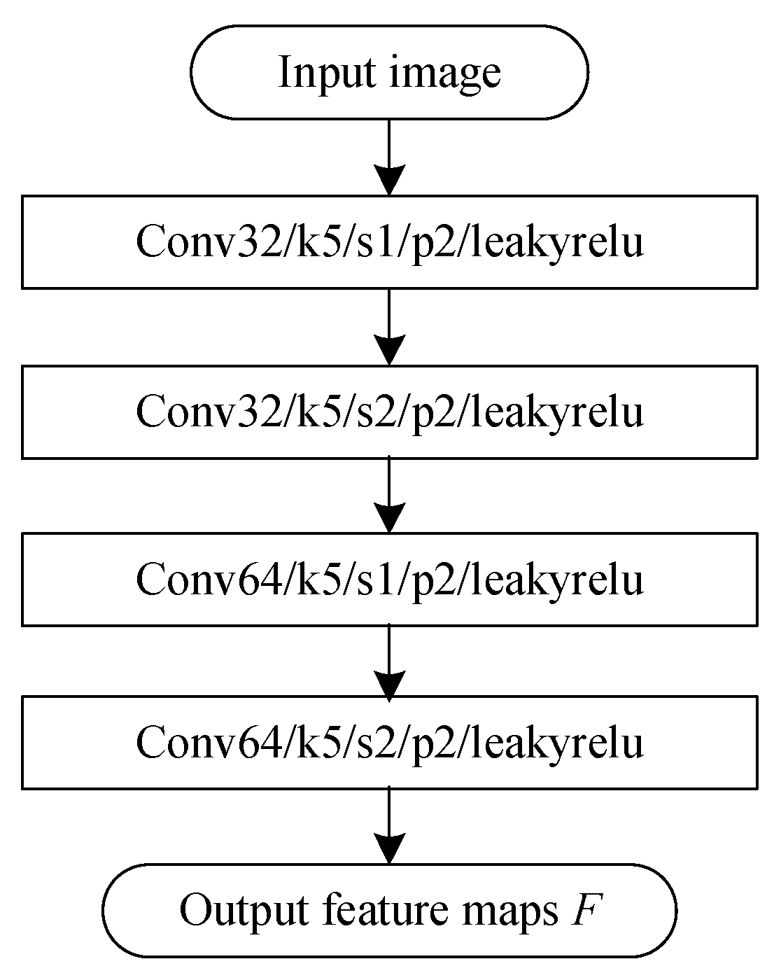
The CNN module aims to map the input sample to the feature map F. The module consists of four convolutional layers and corresponding activation functions. The specific parameters are indicated in Figure 2. For instance, “Conv32/k5/s1/p2/leakyrelu” indicates that the convolution layer has 32 output channels, a kernel size of 5 × 5, a stride of 1, and a padding of 2 around the input. “leakyrelu” refers to the activation function used in this paper, with the slope of the negative half-axis set to 0.1.
Since slot attention employs a structure similar to that of the transformer [47], it does not inherently encode sequential information. In this paper, a position encoding matrix is embedded into the feature map to enhance the positional information of the features. The feature map F has a size of (B, D c n n , H, W), where B is the batch size, D c n n denotes the number of channels and is set to 64, and (H, W) represents the resolution. Next, the position matrix is generated based on the size of the feature map. First, two coordinate axes, x i and y j , are generated as follows:
x i = i H 1 , i [ 0 , H 1 ] y j = j W 1 , j [ 0 , W 1 ]
Then, a four-dimensional position encoding matrix G of size (B,4 , H , W ) is constructed as follows:
G b , 0 , i , j = x i , G b , 1 , i , j = y j , G b , 2 , i , j = 1 x i , G b , 3 , i , j = 1 y j .
where b is batch index ( 0 b < B ). Finally, a linear layer is applied to map the coordinates G to a new shape of (B, D c n n , H, W). As shown in Figure 1, the feature map F of the embedded position matrix is:
F = F + G .

2.3. Slot Attention Module

The slot attention module is the core component of the network proposed in this paper. It disentangles distinct features by associating specific regions of the input samples. The structure of this module is illustrated in Figure 3.
The feature map F is reshaped to serve as the input I to the slot module. The dimension of the input is N × D i , where N represents the number of features and N = H × W , and D i denotes the feature dimension and D i = D c n n . The slot size is set to n × D s , with its values initialized using a Gaussian distribution, where D s represents the feature dimension. In this paper, D s = D c n n is used. Then, a linear layer transforms I and the slot into query Q ( Q R n × D s ), key K( K R N × D s ), and value V( V R N × D s ), as follows:
I l n = f l n K V ( I ) s l o t l n = f l n Q ( s l o t ) Q = f l p Q ( s l o t l n ) K = f l p K ( I l n ) V = f l p V ( I l n )
where f l n refers to layer normalization [48], which enhances the stability of the model by normalizing the input data. I l n ( I l n R N × D i ) and s l o t l n ( s l o t l n R n × D s ) are the result of layer normalization of the input I and slot, respectively. f l p represents a linear map, R denotes the set of real numbers, and the superscripts indicate the matrix dimensions. Next, the similarity matrix M is calculated from the query matrix Q and the key matrix K.
M = Q K T D s .
where M R n × N . Apply the softmax operation along the column dimension of matrix M to obtain the attention matrix a. The formula is:
a i , j = f s ( M i , j ) = e M i , j l e M l , j .
where a R n × N , i , l [ 0 , n 1 ] , j [ 0 , N 1 ] . From the perspective of the matrix’s column dimension, a consists of N attention vectors, each containing n attention coefficients. Each coefficient represents the attention weight among all slots of each input feature, reflecting the degree of attention paid by different slots to the same feature. f s represents the softmax function. The row dimension of the attention matrix is then normalized to obtain A:
A i , j = a i , j l a i , l .
where i [ 0 , n 1 ] , j , l [ 0 , N 1 ] . (7) stabilizes the model’s gradient and facilitates training. From the perspective of the matrix’s row dimension, a represents the attention weight of the query vector across different key vectors, indicating the attention each slot assigns to various features. The value matrix V is weighted using the attention matrix A, resulting in O A V :
O A V = A V .
where O A V R n × D s . In this process, the vectors in V are weighted according to the attention weights, generating new feature representations. Equations (5)–(8) represent the core computational steps of Slot Attention, whose major computational cost arises from the linear interactions between inputs and slots. The time complexity of this process is O ( N · n · D s ) . Since the number of slots n (typically 3–10) is much smaller than the number of inputs N (usually hundreds to thousands), the dominant term O ( N · n · D s ) can be regarded as growing approximately linearly with the input size N in practical scenarios.
(6) and (7) is one of the key factors that enable the slot attention module to perform feature disentanglement. In particular, the softmax function in (6) performs “inter-slot” normalization on the similarity matrix. The softmax function is very sensitive to differences in similarity coefficients. It will amplify the larger value in the input and reduce the smaller value. During the weighted summation process in (8), slots with larger attention coefficients receive more information from the target feature compared to those with smaller coefficients. This reflects the competitive mechanism between the slots. Throughout the weighted summation process, input features are automatically combined, with similar target features aggregated into the same slot and distinct features separated. Ultimately, each slot corresponds to a specific region of the image, facilitating feature disentanglement. However, softmax has a limitation: it reduces smaller values but does not set them to zero, which may result in leakage of target information to different slots. To address this issue, this paper uses a set of feature masks and weights them on the output features, as shown in (9) and (10). Therefore, layer normalization and linear mapping of O A V are performed to obtain O 2 and O 3 :
O 1 = f ln O 1 ( O A V ) , O 2 = f l p O 2 ( O 1 ) , O 3 = f l p O 3 ( O 1 ) .
where O 2 , O 3 R n × D o , D o represents the output feature dimension. In this paper, D o = 256 . Finally, adjust the output features:
O s = O 2 f s ( O 3 ) , f s ( O 3 i , j ) = e O 3 i , j l e O 3 l , j .
where O s R n × D o represents the final output of the module. Combined with the above, O s is the updated slots. ⊙ represents the hadamard product. i , l [ 0 , n 1 ] , j [ 0 , D o 1 ] . f s ( O 3 i , j ) represents the feature mask, which is used to suppress the leaked features and improve the ability of slot separation features. Combining Equations (9) and (10), layer normalization is first applied to eliminate the influence of local energy differences. One linear projection branch preserves semantic features, while the other generates the basis features for attention weights. The softmax operation amplifies the weights of high-response features and suppresses those of low-response features. Finally, by weighting the semantic features, the network adaptively highlights target features with strong energy responses while suppressing background clutter. Overall, through Equations (9) and (10), our network achieves adaptive enhancement and suppression of elements within each slot, enabling secondary decoupling and focusing between targets and background.

2.4. Upsampling Module

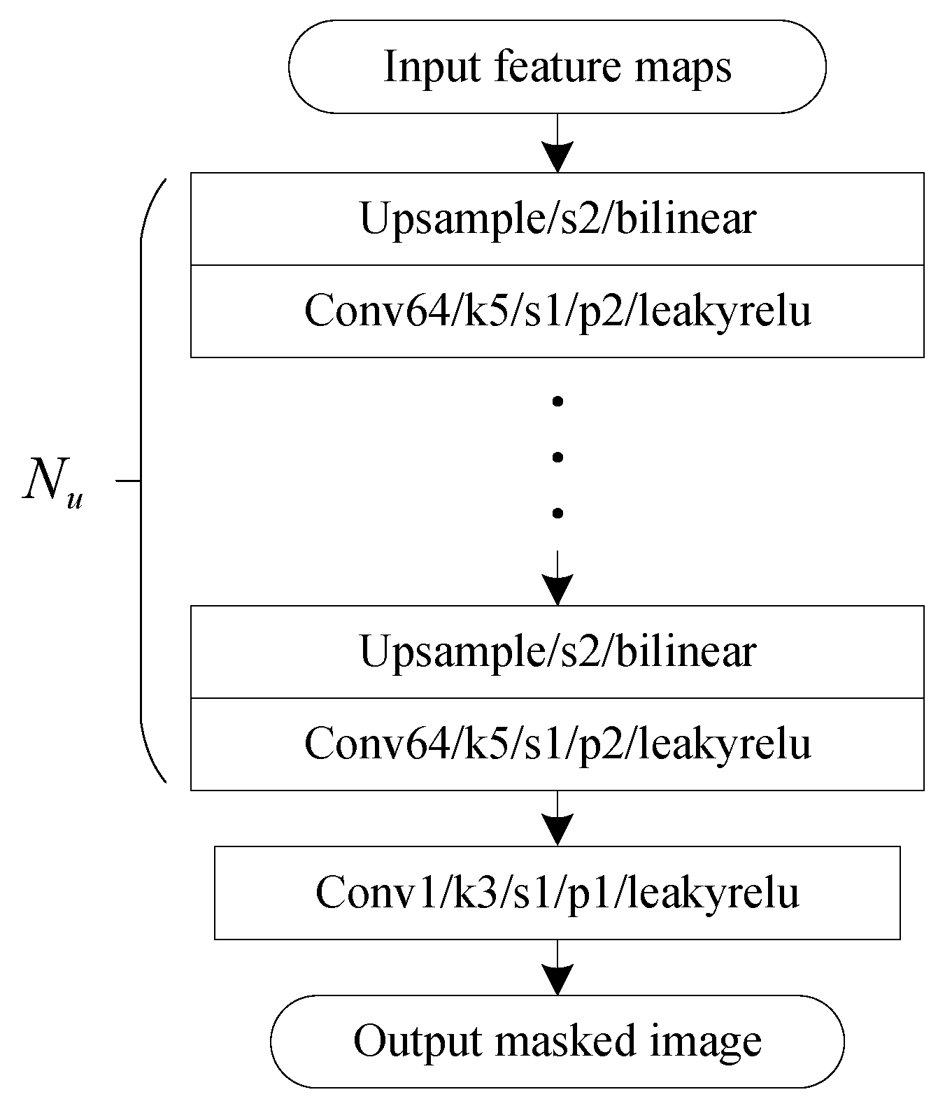
The upsampling module performs the decoder function by reconstructing the encoded features to the original size output image. This module comprises N u upsampling layers and N u + 1 convolution layers. The specific parameters are indicated in Figure 4. For example, “Upsample/s2/bilinear” represents an upsampling layer that performs 2x upsampling using the bilinear interpolation algorithm. The advantage of using the upsampling method over transposed convolution is its ability to avoid the checkerboard effect.
The feature O s is reshaped into I d ( I d R n × H d × W d ), where H d and W d denote the resolution, which is set to 16 in this paper. Next, I d is used as the input to the module. The n feature maps are decoded by the module separately to obtain output image O d ( O d R n × H o × W o ), where H o and W o represent the resolution of the image. H d and H o satisfy H d × 2 N u = H o .

2.5. Slot Selection Module and Classification Module

The slot selection and classification modules are involved in the second-stage classification task. The output O s consists of n features, each corresponding to a specific region of the image. However, due to the black-box nature of neural networks, determining the correspondence between each feature vector and its corresponding image region is challenging. Thus, a specialized module needs to be designed to solve this problem. This step is crucial for strengthening the causal relationship between the target feature and the classification task. This paper thus designs a slot selection module based on the class activation heatmap (CAM) [49]. The design strategy involves treating the slot attention module as an n-classification task, calculating the CAM for each feature, and selecting the slot associated with the target based on the activation region. The steps are:
  • Compute the mean of each feature in O s and calculate the CAM of the first convolutional layer for these n means, resulting in n CAMs. Figure 5 illustrates a schematic of CAM. The four subfigures correspond to the four CAMs generated from the four means when n = 4.
  • Construct a mask matrix M s of size H o × W o . The central region occupying approximately 9% of the total elements (rounded to the nearest integer) is set to 1, while the remaining elements are set to 0. Calculate the total energy C M 1 and C M 2 of different regions of the CAM according to the following formula.
    C M 1 i = ( M s C A M i ) C M 2 j = ( ( 1 H o × W o M s ) C A M j )
    where i , j [ 0 , n 1 ] , C M 1 , C M 2 R n × 1 , ⊙ represents the hadamard product, 1 H o × W o is an all-ones matrix.
  • The features corresponding to the CAMs that satisfy the following conditions are selected as the output of this module.
    C M 1 i > d 1 C M 2 j < ( d 2 × 3 + 5 )
    where i , j [ 0 , n 1 ] , d 1 = 1 in this paper, d 2 = min ( C M 2 ) . The first condition ensures that the central region of the CAM maintains a non-zero energy, thereby filtering out slots unrelated to either the target or the background. The parameter d 2 represents the minimum edge energy of the CAM, and the corresponding slot is considered to be focused on the target. The constants 3 and 5 in the second condition serve as empirical offset terms that relax the CAM response boundary, enabling a more robust slot selection. Finally, if multiple slots satisfy these conditions, their features are summed and output together.
These are all the steps of the slot selection module.
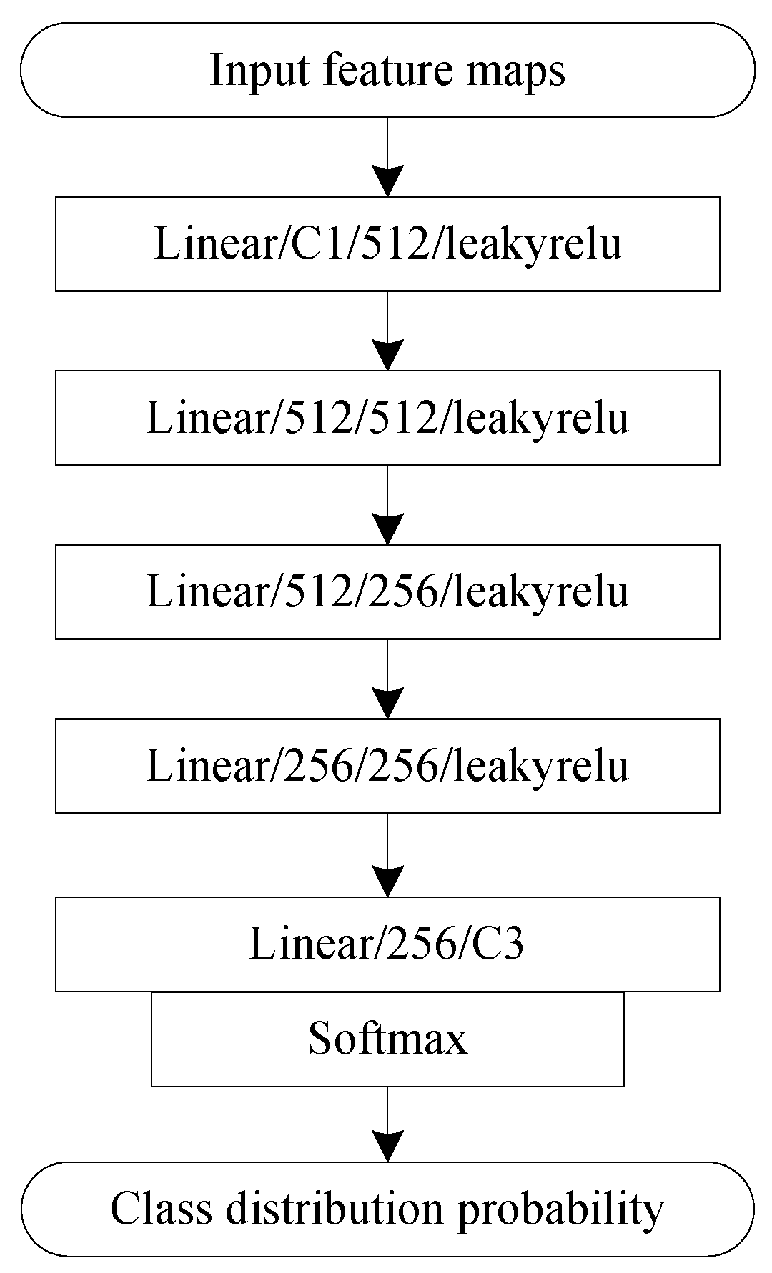
The classification module combines target features and classifies them. The feature vector selected by the selection module serves as the input to this module. This module consists of fully connected layers, with specific parameters shown in Figure 6. For example, “Linear/C1/512/leakyrelu” represents a fully connected layer, with C1 indicating the input feature dimension, 512 indicating the output dimension, and leakyrelu representing the activation function. Finally, the softmax function computes the probability distribution of the output class.

2.6. Loss Function

The two-stage training proposed in this paper optimizes the weights of different modules independently. Therefore, two distinct loss functions are employed to carry out these two training phases. The first loss function is the mean squared error (MSE) loss function, and its formula is:
MSE = 1 N m j = 1 N m | i = 1 n O d ( i j ) L ( j ) | 2 .
where N m denotes the number of samples in a mini-batch, n represents the number of reconstructed outputs for each sample, and L ( j ) is the corresponding reconstruction target. O d ( i j ) ( O d ( i j ) R H o × W o ) represents the i-th reconstructed image of the j-th sample. This is crucial and represents another key factor in determining whether a slot can become competitive. After the convergence of the first loss function, the trainable parameters of the feature extractor are fixed, and the classification network is trained using the second loss function. The second training phase uses the cross-entropy loss function.
CEloss = i = 1 N c y i · ln x i .
where y i represents the one-hot encoding value of the class label conversion, x i represents the output of the network, and N c represents the number of samples.

3. Experimental Results and the Discussion

This section will evaluate the effectiveness and superiority of the proposed network (FDSA-Net) in SAR ATR under cross-background conditions through experiments. First, we introduce the MSTAR dataset [50] and the OpenSARShip dataset [51,52], followed by a description of the experimental settings. Next, we present our experimental results to demonstrate the effectiveness of the network, and finally, we perform comparative experiments to highlight the superiority of the proposed network. The hardware resources for this experiment include an i7-11700 processor, 32GB RAM, and an RTX 2060 GPU with 12GB memory. The software environment consists of Python 3.8 and PyTorch 1.11.0. To assess the robustness of the network, each experimental result is derived by taking the median of five trials.

3.1. Datasets and Experimental Parameter Settings

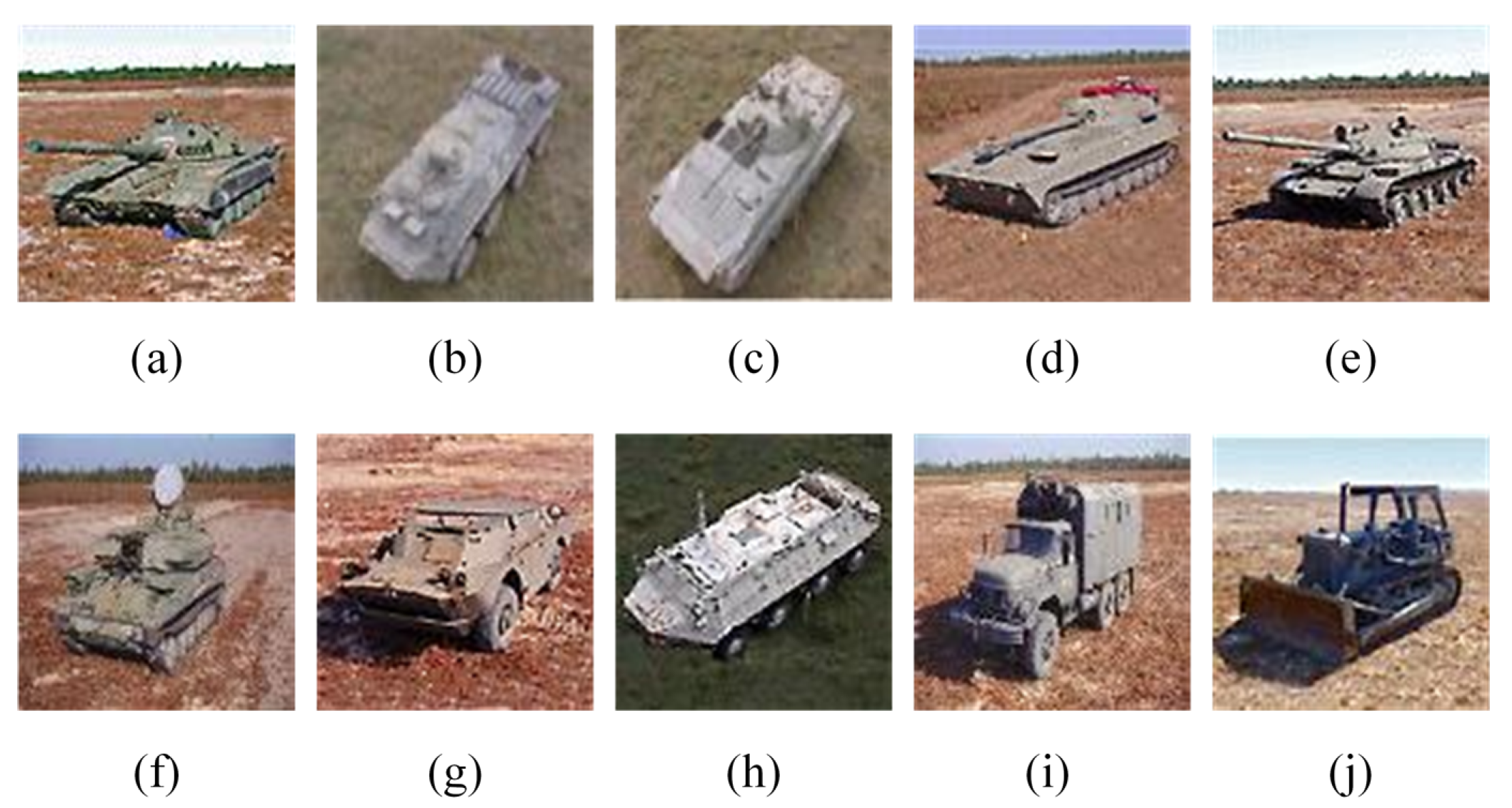
The MSTAR dataset [50] contains SAR images of stationary ground targets captured in real-time, encompassing ten types of civilian and military ground vehicle targets: armored vehicles (BMP-2, BRDM-2, BTR-60, BTR-70), tanks (T62, T72), rocket launchers (2S1), air defense units (ZSU-234), trucks (ZIL-131), and bulldozers (D7). The optical images of these ten target types are shown in Figure 7. The SAR operating mode is X-band, HH polarization spotlight SAR with a resolution of 0.3 m × 0.3 m. The azimuth angles of each target type in the MSTAR dataset range evenly from 0° to 360°. The SOC dataset in MSTAR includes targets with the same serial number and configuration, featuring two pitch angles of 17° and 15°. These dataset can evaluate the network’s recognition performance under slight changes in imaging conditions. Detailed information about the SOC dataset is provided in Table 1.
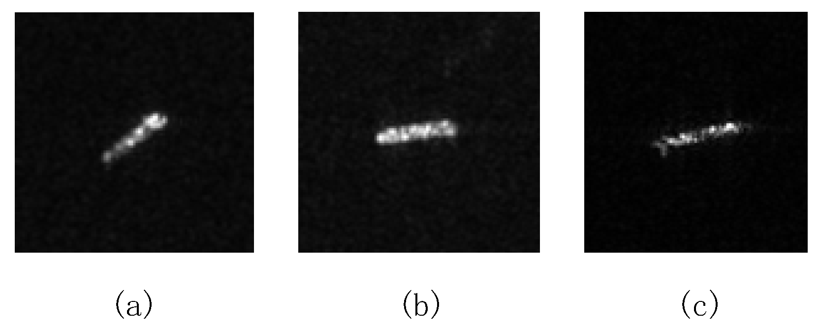
The OpenSARShip dataset [51] consists of satellite SAR data collected by Sentinel-1. The radar operates in the X-band, using VH and VV polarization modes. This paper conducts experiments using three relatively balanced target categories from the OpenSARShip dataset, with their detailed information listed in Table 2. Additionally, Figure 8 presents examples of the SAR samples.
Both datasets contain images with inconsistent brightness, which may introduce bias during model training. Therefore, we apply histogram matching to the images in the datasets. Moreover, since SAR images are single-channel grayscale images, increasing the brightness contrast between the target and the background will help the proposed network better disentangle target and background features. Therefore, during histogram matching, the pixel brightness distribution of the images is adjusted to match that of low-brightness images. Furthermore, to test the robustness of the designed network against background variations, we construct several test datasets with different backgrounds based on (15).
I n = I i M a + G a ( 1 H o × W o M a ) .
where I i represents the image after histogram matching, 1 H o × W o is an all-ones matrix, G a denotes different backgrounds simulated by Gaussian distribution. I n represents the generated new image. M a is a binary segmentation mask of the target region in the image, consisting of values 0 and 1. M a is generated based on the following segmentation method.
First, a brightness enhancement operation is performed on the image I i , producing the output image I o .
I o = I i γ .
where γ = 2.5. The grayscale values are adjusted using a power-law transformation to further enhance the clarity of the target’s edges, which facilitates target segmentation. Then, the Sobel filters S x and S y in the horizontal and vertical directions are applied to compute the edge response strength E of the image I o .
E = ( I o S x ) 2 + ( I o S y ) 2 .
where ⊗ represents two-dimensional convolution.
Finally, the binary segmentation mask M b is generated according to the threshold T:
T = 0.3 · max ( E ) , M b = 1 , if E > T , 0 , if E T .
This thresholding operation means that all positions with an edge response greater than 0.3 times the maximum value of E are assigned to 1, while the remaining positions are set to 0 to form the binary mask. A morphological closing operation is applied to the largest connected component of M b using a circular structuring element with a radius of 5 pixels. This process results in the final binary mask M a . Figure 9 shows an example of input and output images for image segmentation.
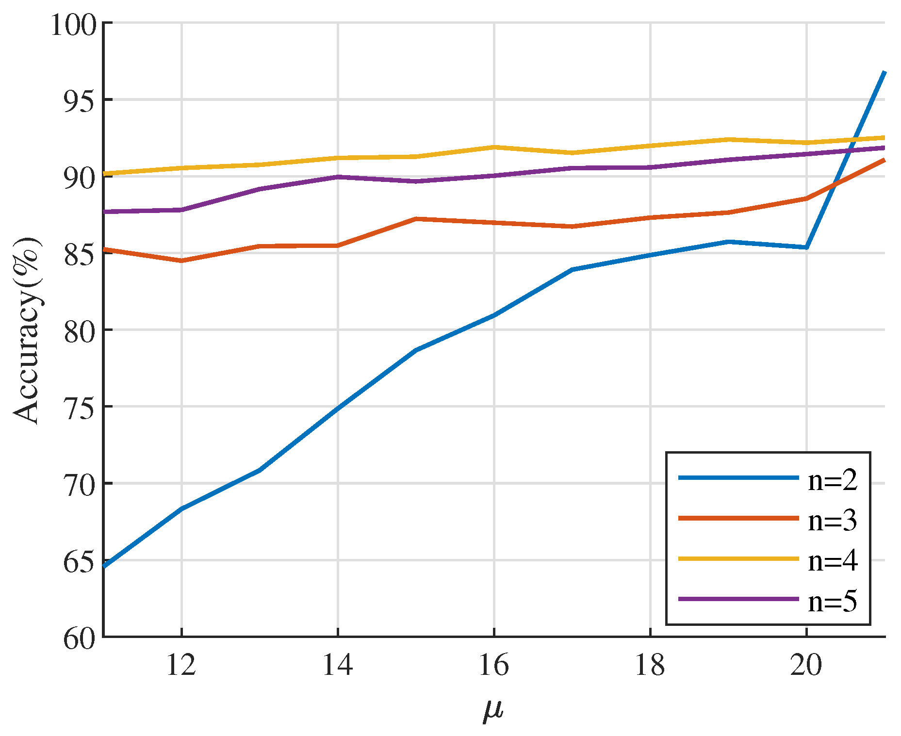
During the training and testing phases, we extracted a 128 × 128 pixel image patch from the center of the original images in the MSTAR dataset. For the OpenSARShip dataset, a 64 × 64 pixel image patch was extracted. No additional data augmentation techniques were applied. In the proposed framework, the weights of the convolutional and linear layers were initialized using a Kaiming uniform distribution [53], while bias vectors were initialized using a uniform distribution. Pre-training was not required. The Adam optimizer [54] was used for weight optimization, with weight decay disabled. The initial learning rate was set to 0.001. The number of epochs for the two training phases were set to 100 and 160, respectively. An early stopping strategy was adopted to prevent overfitting. Specifically, the training was terminated when the magnitude of loss change was smaller than 5 × 10 4 for 20 consecutive epochs. The batch size was set to 32. The classification results were evaluated using accuracy and Shapley values. The method for calculating the Shapley values can be found in the reference [40]. The number of slots n is a critical hyperparameter, as its value significantly affects the network’s ability to achieve optimal feature disentanglement. To investigate this, we conducted a series of experiments on the MSTAR dataset by varying n from 2 to 5 with a step size of 1. According to (15), we constructed datasets with varying background distributions, where the background noise follows a Gaussian distribution N ( μ , σ 2 ) , with μ denoting the mean and σ the standard deviation. Figure 10 presents the recognition accuracy of networks with different n values under various background conditions. The results indicate that the model achieves the best recognition performance when n = 4, suggesting the strongest feature disentanglement capability. Additionally, the models with n = 3 and n = 5 also demonstrate competitive performance, indicating a decent level of disentanglement. The model with n = 5 exhibits lower accuracy than the n = 4 configuration, possibly because a larger number of slots introduces more parameters and increases the risk of overfitting. Considering both effectiveness and stability, we set n = 4 for subsequent experiments.

3.2. Experimental Results on Different Datasets

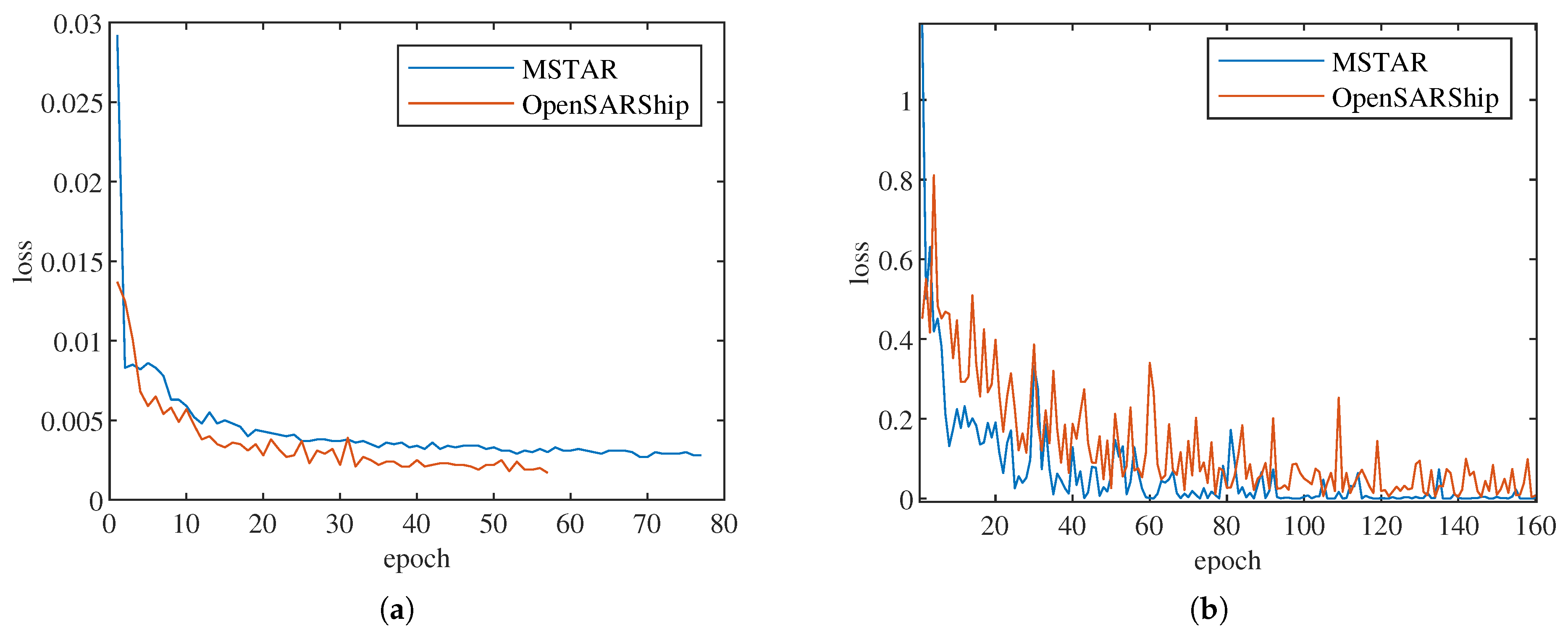
To thoroughly evaluate the performance of the proposed network framework, experiments were conducted on the MSTAR SOC dataset and the OpenSARShip dataset in this subsection. The details of the target names, serial numbers, pitch angles, and sample sizes in the MSTAR dataset are provided in Table 1. As is customary, the samples at a pitch angle of 17° were used for training, while those at 15° were used for testing. The details of the target names and sample sizes in the OpenSARShip dataset are given in Table 2. The loss function curves during the training process are shown in Figure 11.
It can be observed that the loss functions in both training stages of the proposed network reach a minimum and stabilize, indicating that the network has converged. We then evaluate the network’s performance on the original test set. The confusion matrices obtained from the experiments are presented in Table 3 and Table 4. The rows and columns of the table represent “predicted labels” and “ground truths,” respectively.
By analyzing the confusion matrix of Table 3, it is evident that the model performs exceptionally well in most categories, demonstrating the effectiveness of the network in classification tasks. Classes such as BTR-70, BTR-60, BRDM-2, and BMP2 share similar geometric shapes and target characteristics, making them more likely to be confused with one another and resulting in lower accuracy. In contrast, other targets exhibit more distinctive structural features that are easier to identify, leading to higher classification accuracy. The overall classification accuracy reaches 93.88%, indicating that the network can accurately differentiate between different categories and exhibits strong generalization ability.
In Table 4, the network achieves an overall accuracy of 80.39%. The classification accuracy of the Tanker is exceptionally high, reaching 97.44%, with almost no misclassifications. In contrast, the classification accuracy for the Bulk Carrier (80.12%) and Container Ship (75.00%) is slightly lower, primarily due to certain similarities in features between these two categories. However, the overall classification performance remains strong, indicating that the network can effectively distinguish between these three ship types.

3.3. Ablation Experiments

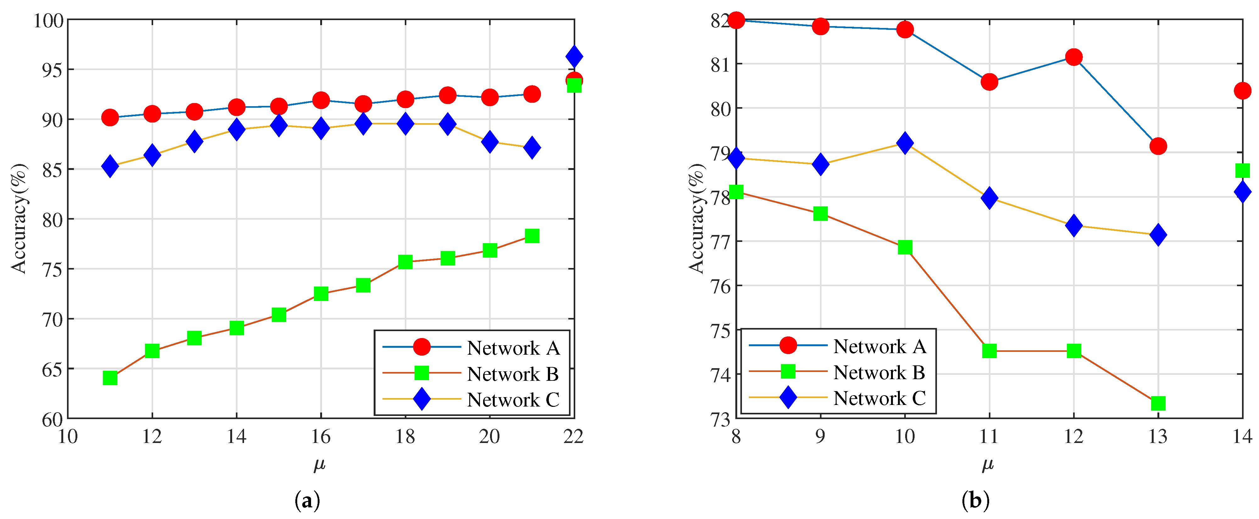
This subsection demonstrates the effectiveness of our proposed innovation through ablation experiments. We denote the complete network designed in this paper as Network A. A variant of Network A, obtained by removing the target mask, is referred to as Network B, which corresponds to the scenario where mask guidance is not applied in the first stage of training. Another variant, obtained by removing the feature mask in the slot attention module, is denoted as Network C. Firstly, we compare the performance of the three networks under different environmental variants. The test set is generated according to (15), where G a N ( μ , σ 2 ) . The experimental results are shown in Figure 12.
Figure 12 illustrates the change in recognition accuracy for networks A, B, and C under different values of μ . It can be observed from the figure that all three networks exhibit fluctuations as the value of μ changes. These fluctuations are mainly caused by random factors during the training process, including weight initialization and the stochastic nature of the optimizer. In addition, MSTAR targets have higher signal energy, making the model less sensitive to background perturbations. In contrast, OpenSARShip targets have lower energy, leading to higher sensitivity to perturbations and a corresponding performance decline. In our experiments, although such fluctuations exist, the overall performance trend remains consistent. The results also show that network A outperforms the two variants. A comparison between network A and network B suggests that the mask guidance makes an independent contribution to the network’s performance. This is mainly because the mask helps the network distinguish between strong clutter points and target features, thereby reducing the impact of strong clutter on performance. A comparison between network A and network C highlights the role of the feature mask in improving performance. This is mainly because the feature mask enhances the ability to disentangle features, thereby improving final recognition performance. Among the three networks, Network B exhibits lower accuracy mainly because the target mask provides useful target-related constraints, and the absence of such information in Network B leads to reduced performance. In summary, the comparison of the three networks demonstrates that the target and feature masks we designed are effective.
Second, the effectiveness of the proposed innovations is further validated by calculating the Shapley values [55] for networks A, B, and C. The Shapley value is a method used to quantify the contribution of each player in a cooperative game. A higher value indicates a greater contribution of the player to the outcome. This is a widely used attribution method [40]. The proposed network primarily decomposes the original image into two parts: the target and the background. These two components are treated as two players, and their respective Shapley values are calculated and subsequently normalized. The normalized results indicate the relative contribution of the target and background to the classification task. The experimental results are presented in Table 5.
From the table, it can be seen that the Shapley values for the target region in the MSTAR dataset (0.9917, 0.93, 0.9869) are much higher than those for the background region (0.0083, 0.07, 0.0131). Similarly, in the OpenSARShip dataset, the Shapley values for the target region (0.9291, 0.8735, 0.81) are significantly higher than those for the background region (0.0709, 0.1265, 0.19). This highlights the dominant influence of the target region on the classification results. These findings indicate that the proposed method effectively focuses on the target region while minimizing the impact of the background, which enhances the network’s recognition ability and robustness across different backgrounds. Additionally, it can be observed from both datasets that the Shapley values for the target region in Network A (0.9917/0.9291) are higher than those of Networks B and C (0.93, 0.9869/0.8735, 0.81). This suggests that incorporating the target mask and feature mask amplifies the contribution of target features to the classification results. This further confirms the important role of the target and feature masks in reducing background interference and improving the network’s target classification ability.
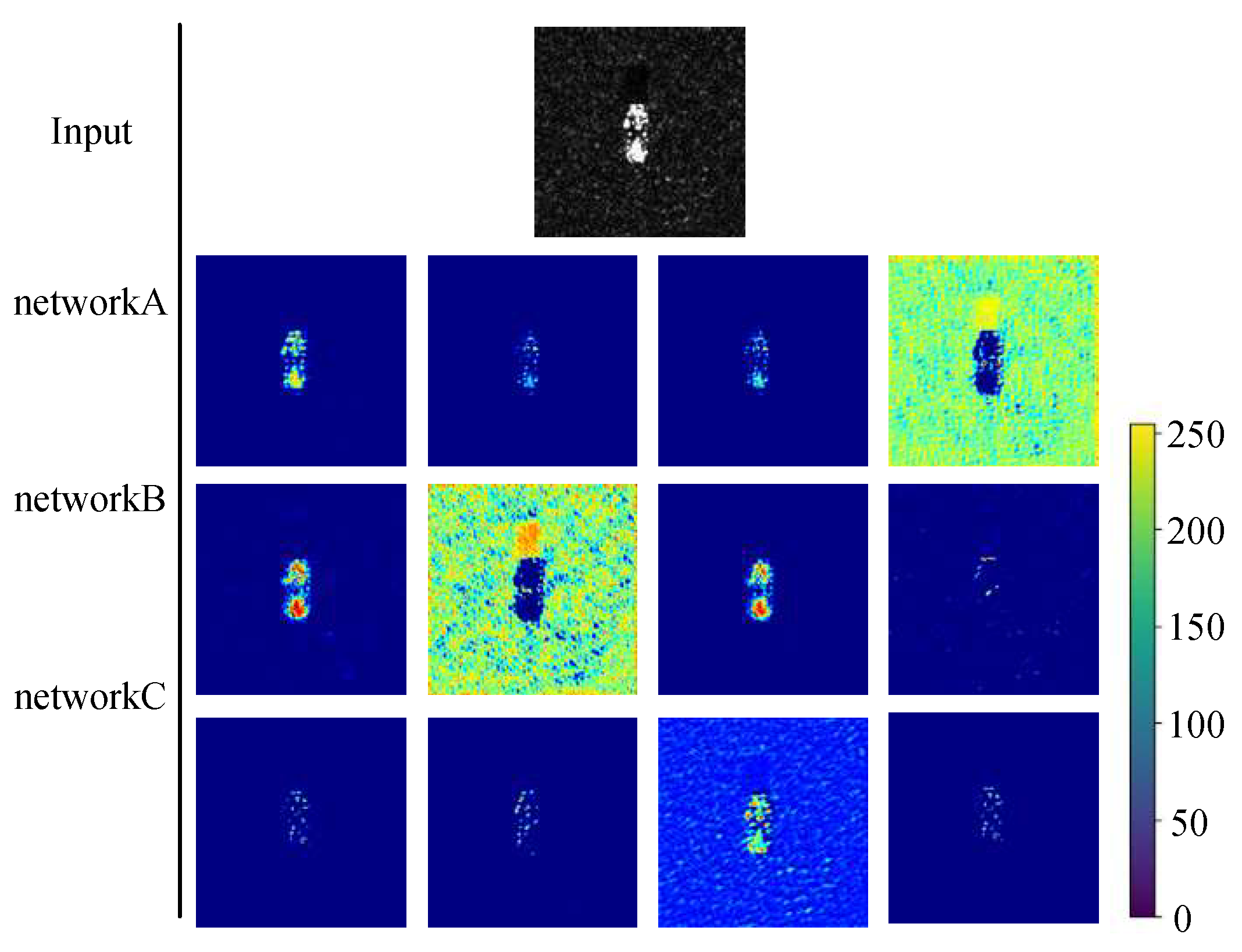
Third, we perform a visualization analysis of the network. CAM provide an intuitive representation of each pixel’s impact on the classification outcome, thereby enhancing the network’s interpretability. In this paper, we treat the slot attention module as an n-class classification task and compute the CAM for each feature in the first convolutional layer. The results are presented in Figure 13.
The first row of Figure 13 shows the input images, while the rows below display the CAMs of the encoders for networks A, B, and C. Each column corresponds to the CAM response of one of the four slots within the network. In the heatmaps, yellow indicates higher activation, and blue represents lower activation. By examining the CAMs for each network, it is evident that the activation areas of the target and background are distributed across different CAMs, suggesting that all three networks are capable of feature disentangling. However, a comparison of the CAMs for networks A and B clearly shows that network A aggregates strong clutter points into the background features, while network B assigns them to the target features. This difference arises because the slot attention mechanism highlights high-intensity regions to aggregate target features. Without the target mask, network B automatically classifies high-intensity clutter and target features as a single category. In contrast, the target mask in network A serves as additional information, helping the slot mechanism distinguish between target features and strong clutter points. This highlights the necessity of using the target mask to guide feature disentangling. As a further comparison, the third CAM of network C shows incomplete feature disentangling, reinforcing the importance of the feature mask. In conclusion, this experiment validates the effectiveness of the proposed design.

3.4. Comparative Experiments

This subsection demonstrates the superiority of our proposed network by designing comparative experiments.
We firstly compare our network with four classic networks: EfficientNet [56], MVGGNet [57], ResNet [58], and A-ConvNet [20]. Among these, EfficientNet and ResNet are widely recognized neural network frameworks in the field of optical images, while A-ConvNet is a well-established benchmark algorithm in the SAR ATR domain. A-ConvNet achieves excellent results by replacing fully connected layers with convolutional layers. MVGGNet is a lightweight variant of VGGNet designed for small-sample SAR ATR. Then, we compare our method with a causal inference framework [45], which represents a state-of-the-art approach in the field of feature disentanglement. We reproduced these five comparison networks based on relevant literature. The input size for A-ConvNet is 88 × 88, and that for the causal framework is 60 × 60, while the other networks use the original image sizes (128 × 128 for MSTAR and 64 × 64 for OpenSARShip). To eliminate the influence of input size on the comparison results, the proposed network was resized to 88 × 88 and 60 × 60 for a fair comparison. To ensure fairness, all networks were trained and tested on a dataset after histogram matching without the use of any data augmentation techniques. The test set consists of two subsets: the original test set (with the original background) and the new test set (with different backgrounds). The recognition accuracy and Shapley values for all networks were obtained through experiments, and the results are presented in Table 6 and Table 7.
The experimental results presented in Table 7 reveal the performance differences in various networks on the original and new test sets. EfficientNet, MVGGNet, and ResNet achieve recognition rates of 97.68%, 99.26%, and 95.45% on the original test set, while their recognition rates on the new test set drop to 42.85%, 8.19%, and 15.22%, respectively. The significant decline in accuracy indicates that these networks exhibit poor generalization ability under different backgrounds. This is primarily due to the large scale of these networks, which makes them prone to overfitting background information during training, while this reduces training error, it leads to over-reliance on specific background features during decision-making, preventing the networks from effectively adapting to new backgrounds. In contrast, A-ConvNet benefits from its smaller size, which reduces overfitting compared to the first three networks, and it achieves a recognition accuracy of 64.19% on the new background dataset. Owing to its capability to eliminate background bias, the causal inference framework achieves a recognition accuracy of 65.75% on the new dataset. As for the network designed in this paper, despite the background change, its accuracy remains relatively high (dropping from 93.88% to 91.98%), demonstrating its strong adaptability to different backgrounds. This performance is attributed to its strong focus on target features and its relatively low reliance on background information. The performance of the proposed network was compared under three different input sizes, and the results show that the input size has little impact on the network’s performance. Table 7 also shows that the performance on the OpenSARShip dataset is significantly lower than that on MSTAR. This discrepancy is primarily attributed to differences in data distribution between the two datasets. Specifically, the MSTAR dataset contains a larger number of samples with azimuth angles collected at nearly uniform intervals, resulting in a more balanced and diverse sample distribution. In contrast, the OpenSARShip dataset has fewer samples and more uneven imaging conditions, leading to weaker generalization and lower recognition accuracy.
From the perspective of Shapley values, EfficientNet and MVGGNet exhibit a balanced reliance on both target and background features, indicating that changes in background features significantly affect their decision-making process. This could be one of the reasons for their poor performance on the new test set. In contrast, ResNet, A-ConvNet and causal framework demonstrate a stronger dependence on target features, with causal framework showing particularly high attention to the target (target Shapley value of 0.9896). The Shapley values for our network reveal an even higher focus on target features (target Shapley value of 0.9917) and a lower reliance on background information. This enables the network to maintain stable performance across different backgrounds, demonstrating superior adaptability to background changes. In addition, the Shapley indicator reflects the degree of feature disentanglement. These values show that background components such as clutter and shadows still have a slight influence on the predictions, while our method maintains the best overall balance between feature disentanglement and classification performance.
A similar conclusion can be drawn from Table 7. Although EfficientNet, MVGGNet, and ResNet outperform our network on the original test set, our network demonstrates the most stable performance on the new test set. Although our network yields lower Shapley values compared to the causal inference framework, it still achieves competitive performance, and attains the highest recognition accuracy on the new background dataset. In conclusion, the comparative experiments validate the superiority of our network in adapting to environmental changes.
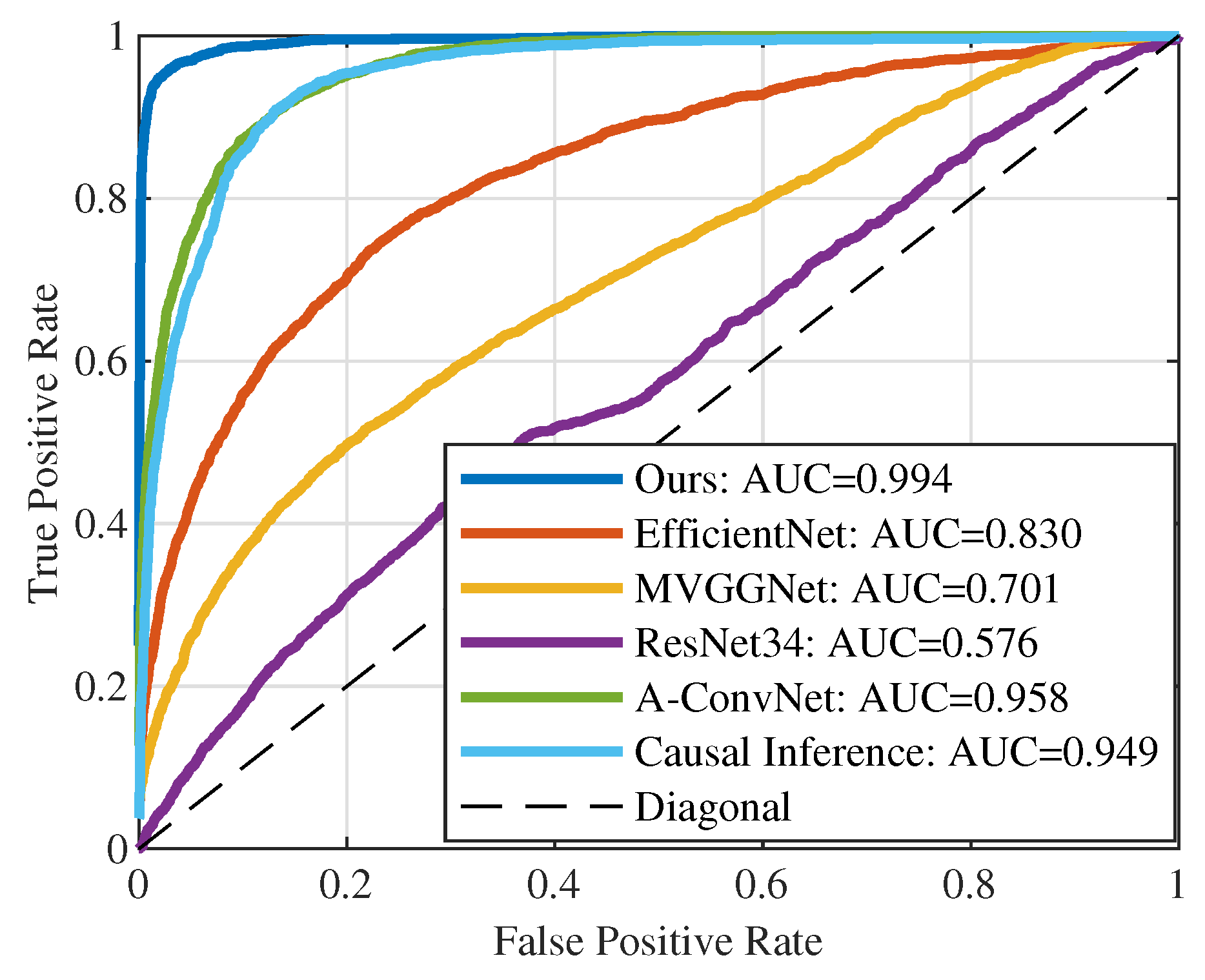
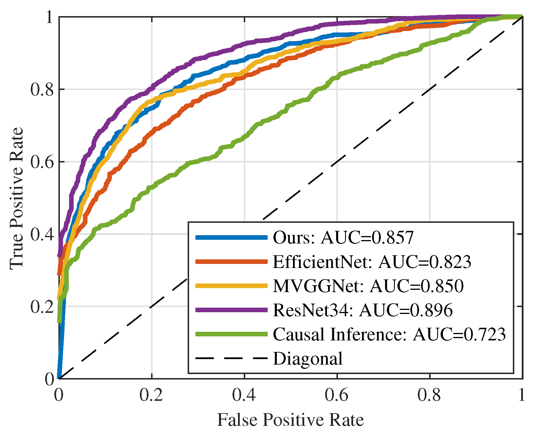
To further evaluate the performance of the proposed network, we plot the ROC curves of our method and several comparison models, as shown in Figure 14 and Figure 15. On the MSTAR dataset, our method achieves the highest AUC of 0.994, with the curve closely approaching the top-left corner, indicating that the network effectively disentangles and captures the discriminative features of targets. The Causal Inference framework and EfficientNet follow with AUCs of 0.949 and 0.830, respectively. In contrast, the curves of ResNet_34 and A-ConvNet exhibit noticeable drops, with significantly lower AUCs of 0.576 and 0.701. On the OpenSARShip dataset, ResNet_34 achieves the best AUC of 0.896, mainly due to its deeper residual architecture that offers slightly better ranking capability. However, this model is less competitive in terms of recognition accuracy and model size. Our method ranks second with an AUC of 0.857. The slight gap to ResNet_34 is primarily attributed to an increase in high-confidence false positives, yet our approach still outperforms other comparison methods by a clear margin. Taken together with the accuracy comparisons presented earlier, these results demonstrate that the proposed network achieves a favorable trade-off between classification accuracy and ranking robustness across cross-background scenarios.

4. Conclusions

This paper proposes a feature disentangling network based on the slot attention mechanism. The network binds target and background features in the input through the mutual competition of n slots. A designed slot selection module is used to identify the slot associated with the target, and the selected slot is then used for the classification task. Additionally, the network’s ability to focus on target features is enhanced by incorporating mask guidance and a feature mask. The proposed network achieves feature disentangling followed by classification, thereby strengthening the causal relationship between target features and classification results.
In future work, we may explore the separation of shadow features and their subsequent fusion with target features to further improve the network’s recognition performance. Another important area for further research is the development of a fast and efficient slot selection module, which is essential for improving the network’s recognition speed. We will further simulate real clutter in future work to improve the experimental fidelity. Our method relies on target masks for weak supervision, which may limit use without segmentation. Future work will explore weaker or self-supervised alternatives to enhance flexibility.

Author Contributions

Conceptualization, T.S.; Methodology, R.W.; Software, R.W. and Y.L.; Validation, R.W.; Formal analysis, R.W.; Investigation, R.W.; Resources, T.S.; Data curation, R.W.; Writing—original draft preparation, R.W.; Writing—review and editing, T.S., Y.L. and J.L.; Visualization, R.W.; Supervision, T.S. and J.L.; Project administration, T.S.; Funding acquisition, T.S. All authors have read and agreed to the published version of the manuscript.

Funding

This work was supported by the National Natural Science Foundation of China under Grant 62271379, and the Innovation Fund of Xidian University.

Institutional Review Board Statement

Not applicable.

Informed Consent Statement

Not applicable.

Data Availability Statement

This paper uses a publicly available dataset, as referenced in [50,52].

Conflicts of Interest

The authors declare no conflicts of interest.

References

  1. Moreira, A.; Prats-Iraola, P.; Younis, M.; Krieger, G.; Hajnsek, I.; Papathanassiou, K.P. A tutorial on synthetic aperture radar. IEEE Geosci. Remote Sens. Mag. 2013, 1, 6–43. [Google Scholar] [CrossRef]
  2. Yu, X.; Yu, H.; Peng, Y.; Miao, L.; Ren, H. Relation-Guided Embedding Transductive Propagation Network with Residual Correction for Few-Shot SAR ATR. Remote Sens. 2025, 17, 2980. [Google Scholar] [CrossRef]
  3. Sun, G.C.; Liu, Y.; Xiang, J.; Liu, W.; Xing, M.; Chen, J. Spaceborne Synthetic Aperture Radar Imaging Algorithms: An overview. IEEE Geosci. Remote Sens. Mag. 2022, 10, 161–184. [Google Scholar] [CrossRef]
  4. Hu, Z.; Xu, D.; Su, T. A Fast Wavenumber Domain 3-D Near-Field Imaging Algorithm for Cross MIMO Array. IEEE Trans. Geosci. Remote Sens. 2024, 62, 1–9. [Google Scholar] [CrossRef]
  5. Hu, Z.; Su, T.; Xu, D.; Pang, G.; Gini, F. A practical approach for calibration of MMW MIMO near-field imaging. Signal Process. 2024, 225, 109634. [Google Scholar] [CrossRef]
  6. Li, Y.; Du, L.; Wei, D. Multiscale CNN Based on Component Analysis for SAR ATR. IEEE Trans. Geosci. Remote Sens. 2022, 60, 1–12. [Google Scholar] [CrossRef]
  7. Leutenegger, S.; Chli, M.; Siegwart, R.Y. BRISK: Binary robust invariant scalable keypoints. In Proceedings of the 2011 International Conference on Computer Vision, Barcelona, Spain, 6–13 November 2011; IEEE: Piscataway, NJ, USA, 2011; pp. 2548–2555. [Google Scholar]
  8. Dalal, N.; Triggs, B. Histograms of oriented gradients for human detection. In Proceedings of the 2005 IEEE Computer Society Conference on Computer Vision and Pattern Recognition (CVPR’05), San Diego, CA, USA, 20–25 June 2005; Volume 1, pp. 886–893. [Google Scholar] [CrossRef]
  9. Clemente, C.; Pallotta, L.; Gaglione, D.; De Maio, A.; Soraghan, J.J. Automatic Target Recognition of Military Vehicles With Krawtchouk Moments. IEEE Trans. Aerosp. Electron. Syst. 2017, 53, 493–500. [Google Scholar] [CrossRef]
  10. Ding, B.; Wen, G.; Zhong, J.; Ma, C.; Yang, X. A robust similarity measure for attributed scattering center sets with application to SAR ATR. Neurocomputing 2017, 219, 130–143. [Google Scholar] [CrossRef]
  11. Mishra, A.K. Validation of PCA and LDA for SAR ATR. In Proceedings of the TENCON 2008—2008 IEEE Region 10 Conference, Hyderabad, India, 19–21 November 2008; pp. 1–6. [Google Scholar] [CrossRef]
  12. Hyvärinen, A.; Karhunen, J.; Oja, E. Independent Component Analysis; John Wiley & Sons: Hoboken, NJ, USA, 2004. [Google Scholar]
  13. Li, X.M.; Sun, Y.; Zhang, Q. Extraction of Sea Ice Cover by Sentinel-1 SAR Based on Support Vector Machine With Unsupervised Generation of Training Data. IEEE Trans. Geosci. Remote Sens. 2021, 59, 3040–3053. [Google Scholar] [CrossRef]
  14. Li, S.; Song, W.; Fang, L.; Chen, Y.; Ghamisi, P.; Benediktsson, J.A. Deep Learning for Hyperspectral Image Classification: An Overview. IEEE Trans. Geosci. Remote Sens. 2019, 57, 6690–6709. [Google Scholar] [CrossRef]
  15. Li, J.; Yu, Z.; Yu, L.; Cheng, P.; Chen, J.; Chi, C. A Comprehensive Survey on SAR ATR in Deep-Learning Era. Remote Sens. 2023, 15, 1454. [Google Scholar] [CrossRef]
  16. Kechagias-Stamatis, O.; Aouf, N. Automatic Target Recognition on Synthetic Aperture Radar Imagery: A Survey. IEEE Aerosp. Electron. Syst. Mag. 2021, 36, 56–81. [Google Scholar] [CrossRef]
  17. Ding, J.; Chen, B.; Liu, H.; Huang, M. Convolutional Neural Network With Data Augmentation for SAR Target Recognition. IEEE Geosci. Remote Sens. Lett. 2016, 13, 364–368. [Google Scholar] [CrossRef]
  18. Guo, J.; Lei, B.; Ding, C.; Zhang, Y. Synthetic Aperture Radar Image Synthesis by Using Generative Adversarial Nets. IEEE Geosci. Remote Sens. Lett. 2017, 14, 1111–1115. [Google Scholar] [CrossRef]
  19. Oh, J.; Kim, M. PeaceGAN: A GAN-Based Multi-Task Learning Method for SAR Target Image Generation with a Pose Estimator and an Auxiliary Classifier. Remote Sens. 2021, 13, 3939. [Google Scholar] [CrossRef]
  20. Chen, S.; Wang, H.; Xu, F.; Jin, Y.Q. Target Classification Using the Deep Convolutional Networks for SAR Images. IEEE Trans. Geosci. Remote Sens. 2016, 54, 4806–4817. [Google Scholar] [CrossRef]
  21. Lin, Z.; Ji, K.; Kang, M.; Leng, X.; Zou, H. Deep Convolutional Highway Unit Network for SAR Target Classification With Limited Labeled Training Data. IEEE Geosci. Remote Sens. Lett. 2017, 14, 1091–1095. [Google Scholar] [CrossRef]
  22. Wang, D.; Song, Y.; Huang, J.; An, D.; Chen, L. SAR Target Classification Based on Multiscale Attention Super-Class Network. IEEE J. Sel. Top. Appl. Earth Obs. Remote Sens. 2022, 15, 9004–9019. [Google Scholar] [CrossRef]
  23. Ren, H.; Yu, X.; Zou, L.; Zhou, Y.; Wang, X.; Bruzzone, L. Extended convolutional capsule network with application on SAR automatic target recognition. Signal Process. 2021, 183, 108021. [Google Scholar] [CrossRef]
  24. Zhang, T.; Zhang, X. Squeeze-and-Excitation Laplacian Pyramid Network With Dual-Polarization Feature Fusion for Ship Classification in SAR Images. IEEE Geosci. Remote Sens. Lett. 2022, 19, 1–5. [Google Scholar] [CrossRef]
  25. Zhang, T.; Zhang, X. A polarization fusion network with geometric feature embedding for SAR ship classification. Pattern Recognit. 2022, 123, 108365. [Google Scholar] [CrossRef]
  26. Pei, J.; Huang, Y.; Huo, W.; Zhang, Y.; Yang, J.; Yeo, T.S. SAR Automatic Target Recognition Based on Multiview Deep Learning Framework. IEEE Trans. Geosci. Remote Sens. 2018, 56, 2196–2210. [Google Scholar] [CrossRef]
  27. Bai, X.; Xue, R.; Wang, L.; Zhou, F. Sequence SAR Image Classification Based on Bidirectional Convolution-Recurrent Network. IEEE Trans. Geosci. Remote Sens. 2019, 57, 9223–9235. [Google Scholar] [CrossRef]
  28. Xue, R.; Bai, X.; Zhou, F. Spatial–Temporal Ensemble Convolution for Sequence SAR Target Classification. IEEE Trans. Geosci. Remote Sens. 2021, 59, 1250–1262. [Google Scholar] [CrossRef]
  29. Lv, B.; Ni, J.; Luo, Y.; Zhao, S.Y.; Liang, J.; Yuan, H.; Zhang, Q. A Multiview Interclass Dissimilarity Feature Fusion SAR Images Recognition Network Within Limited Sample Condition. IEEE J. Sel. Top. Appl. Earth Obs. Remote Sens. 2024, 17, 17820–17836. [Google Scholar] [CrossRef]
  30. Zhang, R.; Duan, Y.; Zhang, J.; Gu, M.; Zhang, S.; Sheng, W. An Adaptive Multiview SAR Automatic Target Recognition Network Based on Image Attention. IEEE J. Sel. Top. Appl. Earth Obs. Remote Sens. 2024, 17, 13634–13645. [Google Scholar] [CrossRef]
  31. Wang, R.; Su, T.; Xu, D.; Chen, J.; Liang, Y. MIGA-Net: Multi-View Image Information Learning Based on Graph Attention Network for SAR Target Recognition. IEEE Trans. Circuits Syst. Video Technol. 2024, 34, 10779–10792. [Google Scholar] [CrossRef]
  32. Zeng, Z.; Sun, J.; Han, Z.; Hong, W. SAR Automatic Target Recognition Method Based on Multi-Stream Complex-Valued Networks. IEEE Trans. Geosci. Remote Sens. 2022, 60, 1–18. [Google Scholar] [CrossRef]
  33. Zhou, X.; Luo, C.; Ren, P.; Zhang, B. Multiscale Complex-Valued Feature Attention Convolutional Neural Network for SAR Automatic Target Recognition. IEEE J. Sel. Top. Appl. Earth Obs. Remote Sens. 2024, 17, 2052–2066. [Google Scholar] [CrossRef]
  34. Liu, Z.; Wang, L.; Wen, Z.; Li, K.; Pan, Q. Multilevel Scattering Center and Deep Feature Fusion Learning Framework for SAR Target Recognition. IEEE Trans. Geosci. Remote Sens. 2022, 60, 1–14. [Google Scholar] [CrossRef]
  35. Xiong, X.; Zhang, X.; Jiang, W.; Liu, T.; Liu, Y.; Liu, L. Lightweight Dual-Stream SAR–ATR Framework Based on an Attention Mechanism-Guided Heterogeneous Graph Network. IEEE J. Sel. Top. Appl. Earth Obs. Remote Sens. 2025, 18, 537–556. [Google Scholar] [CrossRef]
  36. Wen, Z.; Yu, Y.; Wu, Q. Multimodal Discriminative Feature Learning for SAR ATR: A Fusion Framework of Phase History, Scattering Topology, and Image. IEEE Trans. Geosci. Remote Sens. 2024, 62, 1–14. [Google Scholar] [CrossRef]
  37. Huang, Z.; Pan, Z.; Lei, B. What, Where, and How to Transfer in SAR Target Recognition Based on Deep CNNs. IEEE Trans. Geosci. Remote Sens. 2020, 58, 2324–2336. [Google Scholar] [CrossRef]
  38. Li, C.; Du, L.; Du, Y. Semi-Supervised SAR ATR Based on Contrastive Learning and Complementary Label Learning. IEEE Geosci. Remote Sens. Lett. 2024, 21, 1–5. [Google Scholar] [CrossRef]
  39. Belloni, C.; Balleri, A.; Aouf, N.; Le Caillec, J.M.; Merlet, T. Explainability of Deep SAR ATR Through Feature Analysis. IEEE Trans. Aerosp. Electron. Syst. 2021, 57, 659–673. [Google Scholar] [CrossRef]
  40. Li, W.; Yang, W.; Liu, L.; Zhang, W.; Liu, Y. Discovering and Explaining the Noncausality of Deep Learning in SAR ATR. IEEE Geosci. Remote Sens. Lett. 2023, 20, 1–5. [Google Scholar] [CrossRef]
  41. Cui, Z.; Yang, Z.; Zhou, Z.; Mou, L.; Tang, K.; Cao, Z.; Yang, J. Deep Neural Network Explainability Enhancement via Causality-Erasing SHAP Method for SAR Target Recognition. IEEE Trans. Geosci. Remote Sens. 2024, 62, 1–15. [Google Scholar] [CrossRef]
  42. Kang, X.; Guo, J.; Song, B.; Cai, B.; Sun, H.; Zhang, Z. Interpretability for reliable, efficient, and self-cognitive DNNs: From theories to applications. Neurocomputing 2023, 545, 126267. [Google Scholar] [CrossRef]
  43. Zhou, F.; Wang, L.; Bai, X.; Hui, Y. SAR ATR of Ground Vehicles Based on LM-BN-CNN. IEEE Trans. Geosci. Remote Sens. 2018, 56, 7282–7293. [Google Scholar] [CrossRef]
  44. Peng, B.; Xie, J.; Peng, B.; Liu, L. Learning Invariant Representation Via Contrastive Feature Alignment for Clutter Robust SAR ATR. IEEE Geosci. Remote Sens. Lett. 2023, 20, 1–5. [Google Scholar] [CrossRef]
  45. Liu, J.; Liu, Z.; Zhang, Z.; Wang, L.; Liu, M. A New Causal Inference Framework for SAR Target Recognition. IEEE Trans. Artif. Intell. 2024, 5, 4042–4057. [Google Scholar] [CrossRef]
  46. Locatello, F.; Weissenborn, D.; Unterthiner, T.; Mahendran, A.; Heigold, G.; Uszkoreit, J.; Dosovitskiy, A.; Kipf, T. Object-Centric Learning with Slot Attention. In Proceedings of the Advances in Neural Information Processing Systems, Virtual, 6–12 December 2020; Curran Associates, Inc.: Red Hook, NY, USA, 2020; Volume 33, pp. 11525–11538. [Google Scholar]
  47. Vaswani, A.; Shazeer, N.; Parmar, N.; Uszkoreit, J.; Jones, L.; Gomez, A.N.; Kaiser, L.u.; Polosukhin, I. Attention is All you Need. In Proceedings of the Advances in Neural Information Processing Systems, Long Beach, CA, USA, 4–9 December 2017; Curran Associates, Inc.: Red Hook, NY, USA, 2017; Volume 30. [Google Scholar]
  48. Ba, J.L.; Kiros, J.R.; Hinton, G.E. Layer normalization. arXiv 2016, arXiv:1607.06450. [Google Scholar] [CrossRef]
  49. Zhou, B.; Khosla, A.; Lapedriza, A.; Oliva, A.; Torralba, A. Learning deep features for discriminative localization. In Proceedings of the IEEE Conference on Computer Vision and Pattern Recognition, Las Vegas, NV, USA, 27–30 June 2016; pp. 2921–2929. [Google Scholar]
  50. The Air Force Moving and Stationary Target Recognition (MSTAR) Database. Available online: https://www.sdms.afrl.af.mil (accessed on 1 January 2014).
  51. Huang, L.; Liu, B.; Li, B.; Guo, W.; Yu, W.; Zhang, Z.; Yu, W. OpenSARShip: A Dataset Dedicated to Sentinel-1 Ship Interpretation. IEEE J. Sel. Top. Appl. Earth Obs. Remote Sens. 2018, 11, 195–208. [Google Scholar] [CrossRef]
  52. Shanghai Jiao Tong University. OpenSAR: Data and Codes. 2023. Available online: https://opensar.sjtu.edu.cn/DataAndCodes.html (accessed on 15 September 2023).
  53. He, K.; Zhang, X.; Ren, S.; Sun, J. Delving deep into rectifiers: Surpassing human-level performance on imagenet classification. In Proceedings of the IEEE International Conference on Computer Vision, Santiago, Chile, 7–13 December 2015; pp. 1026–1034. [Google Scholar]
  54. Kingma, D.P.; Ba, J. Adam: A Method for Stochastic Optimization. arXiv 2014, arXiv:1412.6980. [Google Scholar]
  55. Shapley, L.S. A value for n-person games. In Contributions to the Theory of Games, Volume II; Princeton University Press: Princeton, NJ, USA, 1953; pp. 307–317. [Google Scholar]
  56. Tan, M.; Le, Q. EfficientNet: Rethinking Model Scaling for Convolutional Neural Networks. In Proceedings of the 36th International Conference on Machine Learning, Long Beach, CA, USA, 9–15 June 2019; PMLR: New York, NY, USA, 2019. Proceedings of Machine Learning Research. Volume 97, pp. 6105–6114. [Google Scholar]
  57. Zhang, J.; Xing, M.; Xie, Y. FEC: A Feature Fusion Framework for SAR Target Recognition Based on Electromagnetic Scattering Features and Deep CNN Features. IEEE Trans. Geosci. Remote Sens. 2021, 59, 2174–2187. [Google Scholar] [CrossRef]
  58. He, K.; Zhang, X.; Ren, S.; Sun, J. Deep Residual Learning for Image Recognition. In Proceedings of the IEEE Conference on Computer Vision and Pattern Recognition (CVPR), Las Vegas, NV, USA, 27–30 June 2016. [Google Scholar]
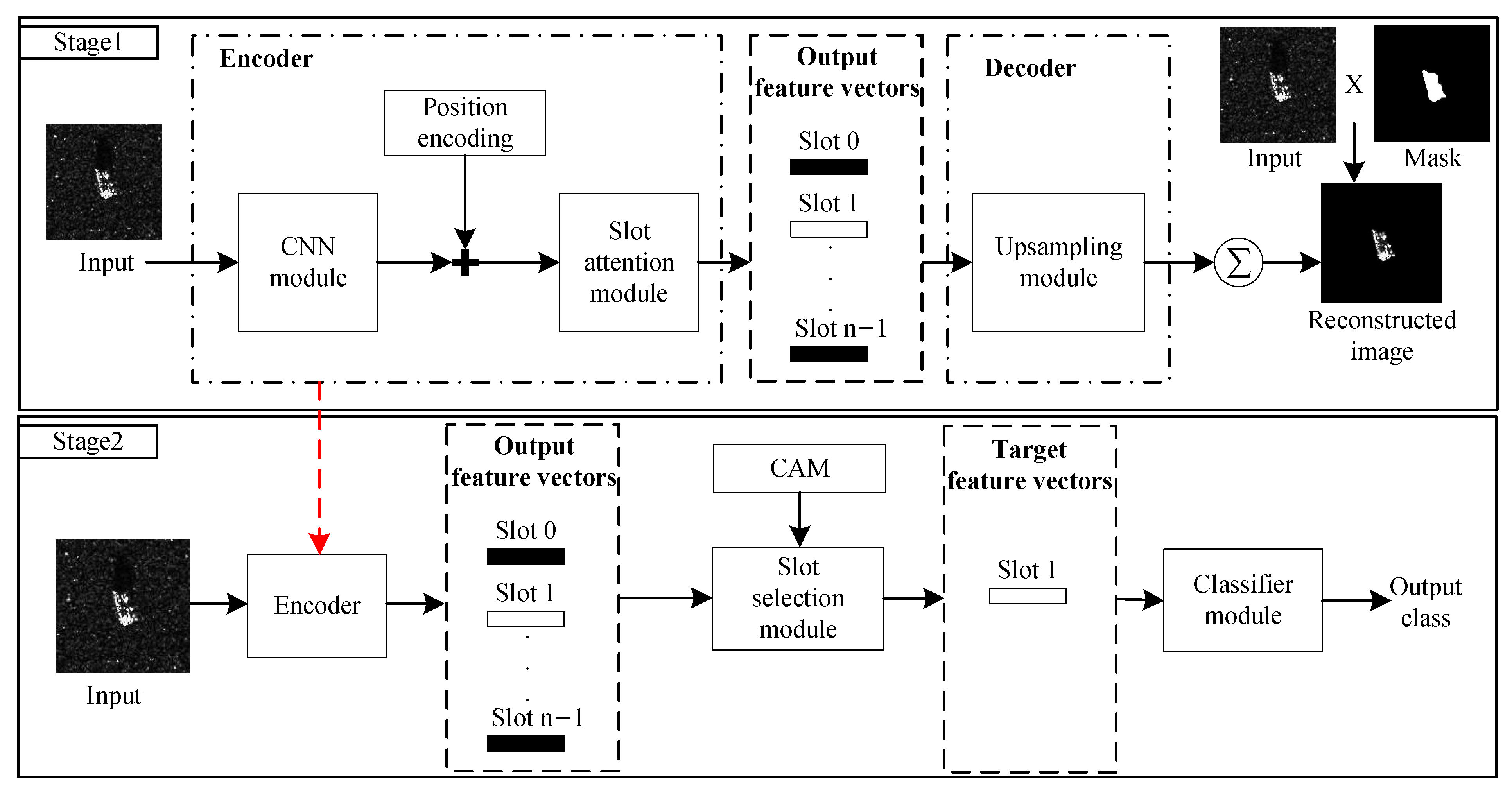
Figure 1. Overall framework of the network.
Remotesensing 18 00003 g001
Figure 2. CNN module.
Remotesensing 18 00003 g002
Figure 3. Slot attention module.
Remotesensing 18 00003 g003
Figure 4. Upsampling module.
Remotesensing 18 00003 g004
Figure 5. Schematic diagram of CAM when n = 4. The activation area of the second CAM is concentrated in the target part, while the rest is in the background part.
Remotesensing 18 00003 g005
Figure 6. Classification module.
Remotesensing 18 00003 g006
Figure 7. Optical sample images of ten types of targets in the MSTAR dataset. (a) T72. (b) BTR-70. (c) BMP2. (d) 2S1. (e) T62. (f) ZSU-234. (g) BRDM-2. (h) BTR-60. (i) ZIL131. (j) D7.
Remotesensing 18 00003 g007
Figure 8. Examples of SAR images in the OpenSARShip dataset. (a) Bulk carrier. (b) Container ship. (c) Tanker.
Remotesensing 18 00003 g008
Figure 9. Image segmentation example. (a) Input image. (b) Binary mask (white 1 black 0). (c) Mask image.
Remotesensing 18 00003 g009
Figure 10. Performance of networks with different values of n under varying background conditions.
Remotesensing 18 00003 g010
Figure 11. Loss function. (a) The loss function of the first training phase. (b) The loss function of the second training phase.
Remotesensing 18 00003 g011
Figure 12. Recognition rates. (a) Recognition rates of networks A, B, and C on the MSTAR dataset. μ increases from 11 to 21, σ = 8. μ = 22 represents the recognition rate of the network in the original test set. (b) Recognition rates of networks A, B, and C on the OpenSARShip dataset. μ increases from 8 to 13, σ = 4. μ = 14 represents the recognition rate of the network in the original test set.
Remotesensing 18 00003 g012
Figure 13. CAM of networks A, B, and C when n = 4.
Remotesensing 18 00003 g013
Figure 14. Comparison of Macro-Average ROC Curves Between Different Models on the MSTAR Dataset.
Remotesensing 18 00003 g014
Figure 15. Comparison of Macro-Average ROC Curves Between Different Models on the OpenSARShip Dataset.
Remotesensing 18 00003 g015
Table 1. Details of SOC.
ClassSerial No.Training SetTesting Set
DepressionNum.DepressionNum.
T72SNS717°22815°191
BTR-70SNc7117°23315°196
BMP2956317°23315°195
BTR-60K10yt753217°25615°195
2S1b0117°29915°274
BRDM-2E-7117°29815°274
D792v1310517°29915°274
T62A5117°29915°273
ZIL131E1217°29915°274
ZSU-234d0817°29915°274
Table 2. Details of OpenSARShip.
ClassTraining Num.Testing Num.
Bulk Carrier1821182
Container Ship182188
Tanker18278
Table 3. Confusion Matrix on SOC Dataset.
ClassT72BTR-70BMP2BTR-602S1BRDM-2D7T62ZIL131ZSU-234Acc. (%)
T7219101110000098.45
BTR-7011655959000085.05
BMP2130172072000088.66
BTR-6046017445000090.16
2S113212661000097.08
BRDM-23118102240000087.59
D700000027301099.64
T6200011002618295.60
ZIL13100007001264296.35
ZSU-23410001024226496.35
Total 93.88
Table 4. Confusion Matrix on OpenSARShip Dataset.
ClassBulk CarrierContainer ShipTankerAcc. (%)
Bulk Carrier947228780.12
Container Ship46141175.00
Tanker117697.44
Total 80.39
Table 5. The Shapley Value of The Target and Background in The Network A,B,C.
Shapley ValueNetworkABC
Player
MSTARBackground0.00830.070.0131
Target0.99170.930.9869
OpenSARShipBackground0.07090.12650.19
Target0.92910.87350.81
Table 6. Comparison of Shapley Value of Each Network on Two Datasets. SvB and SvT represent the Shapley value of the background and target parts, respectively. Our network size refers to the size of the classification subnetwork.
NetworkNetwork
Size
MSTAROpenSARShip
SvBSvTSvBSvT
EfficientNet [56]4.02 M0.46950.53050.45900.5410
MVGGNet [57]16.81 M0.40600.59400.27980.7202
ResNet_34 [58]21.29 M0.20010.79990.25470.7453
A-ConvNet [20]0.30 M0.12230.8777//
Causal [45]0.32 M−0.01040.9896−0.01740.9826
Ours1.03 M0.00830.99170.07090.9291
Ours (88 × 88)0.94 M0.00850.9915//
Ours (60 × 60)0.83 M0.00550.9945//
Table 7. Comparison of Recognition Rates of Each Network on Two Datasets. Original refers to the original test set, while New refers to the newly generated dataset. MSTAR: G a N ( 18 , 8 2 ) . OpenSARShip: G a N ( 8 , 4 2 ) .
NetworkAcc. (%) in MSTARAcc. (%) in OpenSARShip
OriginalNewOriginalNew
EfficientNet [56]97.68%42.85%83.84%79.01%
MVGGNet [57]99.26%8.19%85.70%63.26%
ResNet_34 [58]95.45%15.22%80.66%76.73%
A-ConvNet [20]93.55%64.19%//
Causal [45]68.67%65.75%81.11%79.93%
Ours93.88%91.98%80.39%81.98%
Ours (88 × 88)93.87%92.27%//
Ours (60 × 60)94.17%92.39%//
Disclaimer/Publisher’s Note: The statements, opinions and data contained in all publications are solely those of the individual author(s) and contributor(s) and not of MDPI and/or the editor(s). MDPI and/or the editor(s) disclaim responsibility for any injury to people or property resulting from any ideas, methods, instructions or products referred to in the content.