Article

Online Prototype Angular Balanced Self-Distillation for Non-Ideal Annotation in Remote Sensing Image Segmentation

1
School of Computer Science and Engineering, Macau University of Science and Technology, Macau 999078, China
2
Advanced Institute of Natural Sciences, Beijing Normal University, Zhuhai 519000, China
*
Author to whom correspondence should be addressed.
Remote Sens. 2026, 18(1), 22; https://doi.org/10.3390/rs18010022
Submission received: 12 November 2025 / Revised: 14 December 2025 / Accepted: 15 December 2025 / Published: 22 December 2025
(This article belongs to the Section AI Remote Sensing)

Highlights

That are the main findings?
  • The Online Prototype Angular Balanced Self-Distillation (OPAB) framework enhances remote sensing semantic segmentation performance under non-ideal annotation conditions, reaching 2.0% mIoU improve.
  • The Bilateral-Branch Network (BBN) strategy with a cosine classifier and MMA regularization build an angular balance representation.
  • Stable convergence in label count is observed during OPAB multi-round calibration, ensuring consistent performance.
What is the implication of the main finding?
  • We propose an improved approach to address non-ideal data in remote sensing semantic segmentation, which enhances model generalization.
  • Our modified BBN procedure prevents the performance degradation typically associated with integrating a cosine classifier into an existing code framework.
  • We provide a tool for erroneous label detection and correction. It operates by monitoring the sub-class Local Intrinsic Dimensionality (LID), thereby preventing representation over-compression and the assimilation of erroneous labels in noisy settings.

Abstract

This paper proposes an Online Prototype Angular Balanced Self-Distillation (OPAB) framework to address the challenges posed by non-ideal annotation in remote sensing image semantic segmentation. “Non-ideal annotation” typically refers to scenarios where long-tailed class distributions and label noise coexist in both training and testing sets. Existing methods often tackle these two issues separately, overlooking the conflict between noisy samples and minority classes as well as the unreliable early stopping caused by non-clean validation sets, which exacerbates the model’s tendency to memorize noisy samples. OPAB mitigates the imbalance problem by employing an improved bilateral-branch network (BBN) that integrates max-min angular regularization (MMA) and category-level inverse weighting to achieve balanced hyperspherical representations. The balanced hyperspherical representations further facilitate noise-clean sample separation and early stopping estimation based on large category-wise Local Intrinsic Dimensionality (LID). Moreover, OPAB introduces a bootstrap teacher label refinement strategy coupled with a student full-parameter retraining mechanism to avoid memorizing noisy samples. Experimental results on ISPRS datasets demonstrate that OPAB achieves a 2.0% mIoU improvement under non-ideal annotation conditions and achieves 89% mIoU after cross-set correction, showcasing strong robustness across different backbones and effective iterative calibration capability.

1. Introduction

Remote sensing image semantic segmentation faces the core challenge of intertwined long-tailed class distribution and label noise, which significantly impacts critical applications such as urban planning [1,2,3,4,5] and environmental monitoring [6,7,8,9,10]. In pixel-level classification tasks, the long-tailed distribution manifests as a considerably larger number of pixels in certain dominant categories (e.g., roads, buildings) compared to rare categories (e.g., specific vegetation types, small objects), leading to a notable decline in model recognition performance for rare classes. Noisy labels primarily stem from coarse-grained annotations and crowdsourced data collection processes and are particularly prevalent in class boundary regions and categories with scarce samples [11,12]. This issue shares a similar formation mechanism with annotation noise in medical image segmentation caused by the scarcity of high-quality annotations, both of which significantly impair the model’s generalization capability [13], shown in Figure 1.
Existing research methods typically address these two issues separately: During training, re-weighting methods [22,23,24] alleviate class imbalance by adjusting the weights of samples from different categories in the loss function, whereas noise-robust learning [25,26,27,28,29,30,31,32] methods mitigate the negative impact of noisy labels by introducing regularization constraints or designing robust loss functions. To tackle the synergistic interference caused by long-tailed distributions and label noise, current distillation studies [11,33,34,35,36] have proposed various strategies, but they generally target each problem individually. The ACOC-MT framework performs object-level label correction using adaptive confidence thresholds [11]; knowledge distillation methods introduce noise to generate diverse teacher perspectives [24,32,34,35]; and clear validation dataset loss monitors the early learning phase to avoid memory noisy annotations [37]. However, in teacher–student frameworks, class imbalance leads to significant bias in pseudo-labels generated by the teacher for tail classes, resulting in representation collapse [38]. Meanwhile, noise memorized in head classes propagates to the student model through pseudo-labels, causing cumulative errors. Early-stopping strategies [37,39,40] typically terminate training based on validation loss minimization, but under non-ideal conditions, the validation loss may be corrupted, causing the model to stop at a solution yet overfit to noisy patterns. In such cases, the teacher model can also introduce erroneous labels into the distillation process [11,35,36]. Furthermore, the synergistic effect of long-tailed distributions and label noise exacerbates gradient interference, whereby the optimization directions of rare classes are dominated by noisy gradients from majority classes, making retraining strategies indispensable in the distillation process.
To address the intertwined challenges of non-ideal data, specifically imbalanced class frequencies and label noise, we propose the Online Prototype Angular Balanced Self-Distillation (OPAB) framework. Although existing teacher-student methods have shown promise in knowledge distillation [34] and noisy label learning [13,34,41], they often overlook the need for explicit geometric constraints to handle class imbalance. Building upon the concept of balanced hyperspherical representation inspired by Minimizing Hyperspherical Energy [42,43] and the Lipschitz continuity assumption [44], the OPAB framework introduces three key innovations. First, OPAB incorporates a modified bilateral-branch network (BBN) [45] with category-level inverse weighting to address class imbalance. Second, OPAB employs Maximizing Minimal Angles (MMA) regularization [46] to enforce angular separation between class prototypes on the unit hypersphere. Third, OPAB replaces conventional early stopping with a selection criterion based on large category-level Local Intrinsic Dimensionality (LID) [28,47], synchronizing teacher model weights for the self-distillation step. During the self-distillation training phase, the student model is fully reinitialized to avoid memorizing noisy labels from previous stages.
Our Online Prototype Angular Balanced Self-Distillation (OPAB) framework integrates three technical innovations to tackle class imbalance and label noise in semantic segmentation. First, we employ a modified bilateral-branch network [45] with category-level inverse weighting, which dynamically scales loss contributions according to class frequency, effectively preventing representation collapse in tail classes. Second, we borrow the idea of Maximizing Minimal Angles (MMA) regularization [46] for representation learning, which enhances inter-class discrimination by enforcing angular separation between class prototypes on the unit hypersphere, thereby reducing class overlap. Third, we replace validation-loss-based early stopping with category-level Local Intrinsic Dimensionality (LID) [28] monitoring to address the challenge of non-clean validation sets. We hypothesize that a correctly learned model adheres to Lipschitz continuity—i.e., outputs for the same class do not change abruptly, and embedded pixel vectors of the same category belong to the same cluster. Therefore, during training with confirmed label noise, a high category-level LID may indicate that the model has learned correct representations, meaning mislabeled pixel vectors are embedded within their correct clusters.
In summary, this paper addresses the challenging problem of joint long-tailed class distribution and label noise in remote sensing semantic segmentation, where conventional methods typically treat these issues separately. To address the challenge of label noise in remote sensing, experiments incorporate a novel validation protocol. This protocol, inspired by cross-validation, alternates between training and refining both the training and validation sets, without altering the test set. As a result, our approach improves mIoU by up to 2.0%, reaching 89% after cross-set correction. Our main contributions are summarized as follows:
  • We propose a unified teacher-student framework that leverages geometric and manifold learning principles to simultaneously handle both long-tailed distributions and noisy labels.
  • We introduce balanced hyperspherical representations regularized by a Maximizing Minimal Angles (MMA) objective, along with category-level Local Intrinsic Dimensionality (LID) monitoring. This design enhances inter-class separability and enables effective detection of label noise, without reliance on potentially contaminated validation metrics.
  • We develop a stopping criterion based on category-level LID trends to prevent noise memorization. By tracking changes in local manifold structure, our method overcomes the limitations of validation-loss-based stopping strategies.
  • Extensive experiments on benchmark datasets demonstrate consistent performance gains. The proposed approach achieves an average improvement of 2.0% in mIoU across varying noise levels and class distributions, while showing notable robustness against representation collapse in tail classes.

2. Related Work

2.1. Long-Tailed Semantic Segmentation

In remote sensing semantic segmentation, land-cover categories typically exhibit a long-tailed distribution, where classes such as buildings and roads have abundant samples, while small objects (e.g., ships, towers) are scarce. Such imbalance often biases models toward head classes, degrading the recognition performance of tail classes. Existing approaches mainly include re-weighting [22,23,24], resampling [48,49], and data augmentation [50]. However, in the presence of noisy annotation [23], these long-tail strategies can be significantly compromised: re-weighting may amplify the influence of mislabeled samples, resampling can repeatedly expose noisy tail samples, and data augmentation may generate synthetic data containing label noise [13]. Consequently, the effectiveness of standard long-tailed techniques is highly sensitive to annotation noise, highlighting the need for methods that can jointly address class imbalance and label corruption.
Self-distillation has been introduced into remote sensing segmentation to mitigate noise interference. Its performance improvements mainly arise from the implicit denoising and boundary-smoothing effects provided by soft labels. However, relying solely on soft labels may be insufficient to effectively handle long-tailed distributions under noise and class bias conditions [36]. In other words, although soft labels can alleviate noise interference to some extent, stronger boundary constraints and class-balancing strategies are still required to enhance robustness in long-tailed scenarios. Moreover, incorporating Minimizing Hyperspherical Energy (MHE) regularization [42,43] helps maintain the feature diversity of tail classes, prevent feature collapse, and provide geometric constraints for boundary stabilization. Overall, a self-distillation framework that integrates dynamic label correction and teacher–class balancing mechanisms demonstrates greater robustness for long-tailed semantic segmentation [13].

2.2. Noisy Label Learning in Remote Sensing Segmentation

When transferring noisy label learning from image classification to remote sensing semantic segmentation, the noise characteristics become more complex due to multi-scale objects, visually similar land-cover categories, and blurred boundaries. Conventional methods, such as MentorNet [51] and Co-teaching [32], which rely on sample-level loss ranking or consistency constraints, struggle to handle shape noise caused by boundary errors and semantic noise induced by category confusion [40]. Regularization strategies, such as label smoothing [52,53] and MixUp [54,55], can mitigate noise to some extent but tend to weaken tail class representations under long-tailed distributions. The performance degradation is primarily attributed to the spatial heterogeneity of pixel-level noise, the strong reliance of segmentation models on local context, and the intricate coupling between long-tailed distributions and label noise [11]. To address these issues, various pixel-level noise-robust frameworks have been proposed in recent years: BAKD suppresses noise through boundary uncertainty estimation [12]; Double Similarity Distillation strengthens semantic consistency via inter-class similarity distillation [56,57]; AIO 2 integrates object-level correction with temporal adaptive mechanisms [40]; and ACOC-MT leverages contextual invariance and adaptive thresholding to improve prediction stability [11]. Notably, standard self-distillation approaches generally adopt a two-stage strategy for noise mitigation: the first stage focuses on teacher model soft-label generation, while the second stage trains the student model under guidance from the teacher’s soft labels, gradually suppressing noise and enhancing tail class representations.
Under conditions without a clean validation set, traditional early stopping strategies based on validation loss are prone to overfitting noisy labels. To address this, we introduce a dynamic stopping mechanism inspired by the Lipschitz continuity hypothesis [44] and pixel representation clustering assumptions [58]. When the model has not memorized incorrect labels, erroneous labels tend to cluster with their correct class, resulting in high Local Intrinsic Dimensionality (LID) statistics. We leverage large LID values as the stopping criterion for the first stage of the two-stage training. In the second stage, the student model continues self-distillation under the teacher’s soft-label guidance, combined with dynamic label correction and class-weight rebalancing, thereby mitigating noise effects and improving tail class generalization even in the absence of a clean validation set.

3. Methods

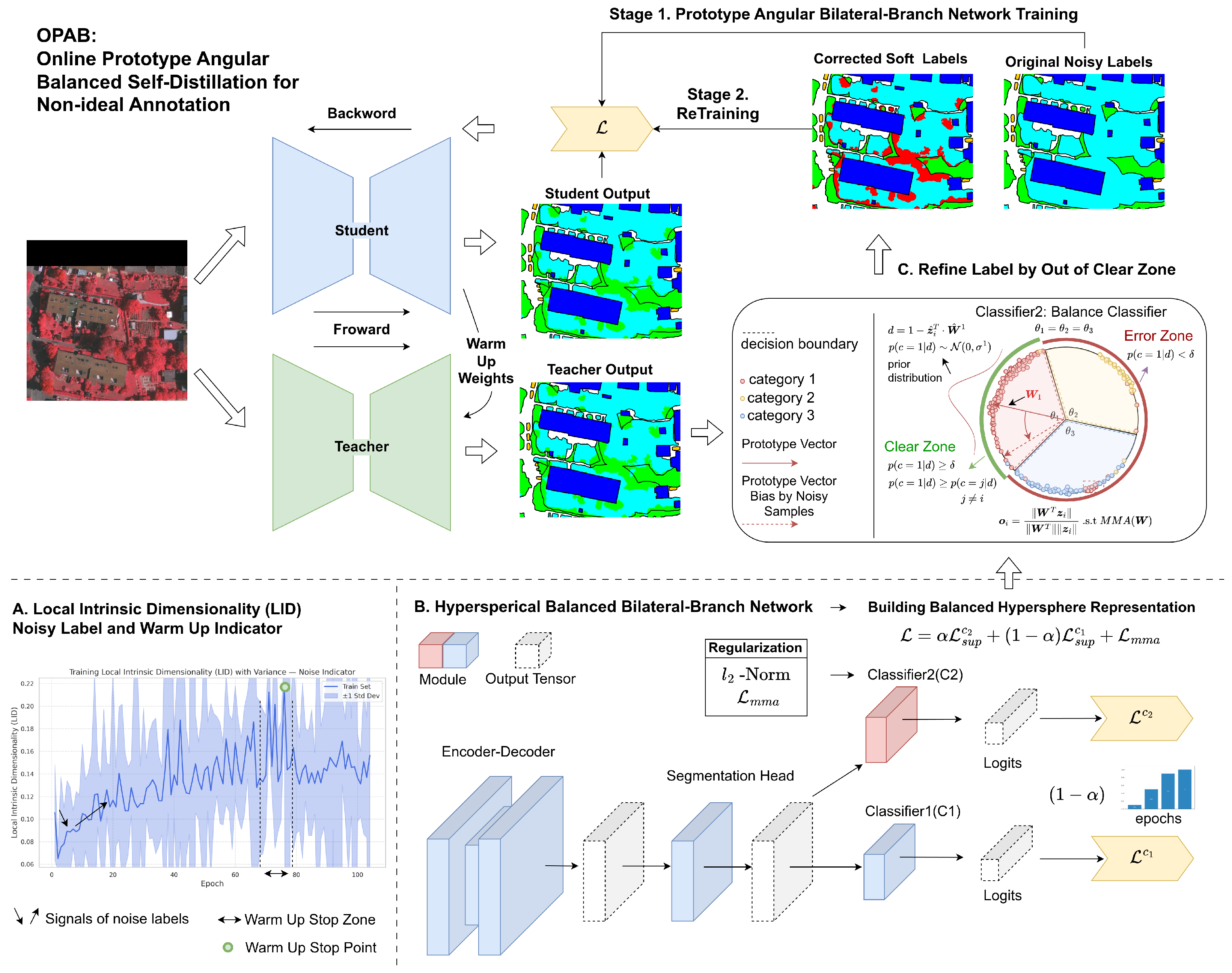
To address long-tailed and noisy segmentation, we propose Online Prototype Angular Balanced Self-Distillation (OPAB), a two-stage teacher-student framework: the first stage performs warm-up training on noisy data, and the second stage refines noisy labels with pseudo-labels for retraining. Specifically, we modify the bilateral-branch network (BBN) [45], where the default branch follows standard training, and the balancing branch applies MMA [46] directly to the classifier, promoting angular separation among class prototypes.

3.1. Semantic Segmentation Framework Design Based on a Bilateral-Branch Network

To address the coupled issues of long-tailed distributions and label noise in remote sensing image semantic segmentation, we propose an improved bilateral-branch network (BBN) framework, detail in Figure 2 part B. Our modified BBN framework consists of a default branch and a balanced branch: the default branch employs the standard cross-entropy loss to handle all training samples, while the balanced branch specifically optimizes tail classes through a class-level inverse weighting mechanism. For the first branch, we use a linear classifier, denoted as c 1 , while for the second branch, we adopt a cosine classifier, denoted as c 2 . The main loss of our modified BBN framework is defined as follows:
L = α · L s u p c 1 + ( 1 α ) · ω b · L s u p c 2 + β · L m m a .
Our main loss guides the model to transform its learned representations from unconstrained forms into hyperspherical representations. α and β are the hyperparameters for the main loss, as discussed in Section 5.3. In detail, α is a weighting factor that controls the relative importance of the losses between the two classifiers. As training progresses, α gradually decreases from its initial value of 1 to 0, causing the model’s emphasis to shift from classifier c 1 to classifier c 2 . This process also imposes a reverse constraint, encouraging the learned representations to align with the expectations of the classifiers. β is the hyperparameter for the MMA [46] loss of classifier c 2 . L mma is the max–min angular regularization applied to c 2 , described in Section 3.2. ω b is a category-level inverse weighting [23], which is used to amplify the loss signal of minority classes.
The cross entropy loss denoted as L s u p and the output probability distribution as p = p 1 , p 2 , , p K . Each prediction, p , corresponds to a one-hot label y = y 1 , y 2 , , y K . Then, the supervised loss is defined as
L s u p = k = 1 K y k l o g ( p k ) + ( 1 y k ) l o g ( 1 p k ) .

3.2. Balanced Hyperspherical Representations and Max-Min Angular Regularization

Our bilateral-branch network architecture proposes a method for building balanced hyperspherical representations with max-min angular regularization [46] to optimize the geometric relationships among class prototypes. This method constrains the feature space to the unit hypersphere S d 1 , where all class prototype vectors w ^ i c 2 satisfy the normalization condition: w ^ i c 2 2 = 1 . Let the total number of classes be n. To achieve maximal inter-class separation, we define the max-min angular regularization term as
L mma = 1 n i = 1 n min j i θ i j , θ i j = arccos w ^ i c 2 · w ^ j c 2 ,
where θ i j denotes the angular distance between class prototypes i and j. This regularization encourages the class prototypes to approach a uniform distribution on the hypersphere by maximizing the minimal angular distance between any two prototypes. The latent representation of each sample i, denoted as z ^ i S d 1 and z ^ i 2 = 1 , is constrained to remain close to its corresponding class prototype. Once the class prototypes are uniformly distributed, tail-class prototypes gain sufficient angular space on the hypersphere, allowing their sample representations to spread out without being compressed or collapsed by other classes. This mechanism effectively mitigates the collapse problem of tail-class representations under long-tailed distributions.

3.3. Label Correction via Hyperspherical Angular Bisectors

From a geometric perspective, distinguishing clean samples from noisy labels on the hypersphere mainly requires defining a decision boundary for clean samples and noisy samples. This usually involves evaluating an angular threshold for each class and performing additional clustering on the learned class representations. To simplify distinguishing clean samples from noisy labels, we propose using the angular bisector in the hyperspherical balanced representation as a unified boundary between clean and noisy samples.
Assume that for each category in the ideal balanced state, the representations are distributed around the class prototype with equal-variance Gaussian distribution. Based on this assumption, we innovatively unify the classification decision boundary and the clean-noise separation boundary: The angular bisector between any two class prototypes simultaneously serves as both the decision boundary for distinguishing clean and noisy samples and the classification boundary, and samples crossing this boundary are considered potential mislabeled samples; detailed proof can be found in Supplementary Section S1.
Formally, as the latent representation of any sample i is z ^ i S d 1 in k category, we define the error zone as
I k error zone = z ^ i S d 1 : arccos ( w ^ k T z ^ i ) > θ threshold ,
where θ threshold is a preset angular threshold to identify noisy samples deviating from the class prototype. In the hyperspherical balanced representation, this threshold corresponds to the angular bisector,
θ threshold = arccos 1 + w ^ k T w ^ j 2 ( 1 + w ^ k T w ^ j ) ,
where w ^ k and w ^ j denote the learnable weight vectors as class prototypes of classes k and j, respectively, and category j denotes any category except k in the classification task.
To further address label noise, we introduce a hybrid label correction mechanism based on balanced hypersphere geometry. By measuring the angular deviation between a sample and its class prototype, potential mislabeled samples are identified. For a sample i and class prototype w ^ k , the error zone I k error zone and clear zone I k clear zone are defined as
I k error zone = i   |   1 w ^ k T z ^ i < 1 + w ^ k T w ^ j 2 ( 1 + w ^ k T w ^ j ) ,
I k clear zone = i   |   1 + w ^ k T w ^ j 2 ( 1 + w ^ k T w ^ j ) w ^ k T z ^ i < 1 .
Consistent with unsupervised label error detection [59,60], we update labels using the bootstrapping method, defined as
y ˜ i = ω i y i * + ( 1 ω i ) y ˜ i ,
where y ˜ i is the original true label one-hot vector, and y i * is the teacher model’s predicted label one-hot vector. The weight ω i for the i-th sample in class k is defined as
ω i = 1 , i I k error zone , 0 , otherwise .

3.4. Warm Up Strategy

To improve teacher quality and improve noise-clean separation, we modify Local Intrinsic Dimensionality (LID) at the category level as an early stopping criterion. Our approach targets high category-level LID to better separate noisy and clean samples. The class-wise Local Intrinsic Dimensionality (LID) is defined as
LID category level ( x ) = 1 j i = 1 j 1 k j i = 1 k j log r i ( x ) r k ( x ) 1 ,
where r i ( x ) is the distance to the i-th nearest neighbor of data point x . A high category-level LID implies low intra-class cohesion, which improves the discernibility between noisy and clean samples. However, high category-level LID also indicates greater overlap between class representations, potentially leading to misclassification errors. The balanced hyperspherical representation further alleviates overlap-induced issues by maximizing inter-class prototype distances while maintaining equitable feature space partitioning. To overcome the representation overlap while accounting for potential bias in the teacher model, we completely re-initialize and retrain the student model in the second stage, rather than fine-tuning from the teacher parameters. The second-stage training adopts validation loss as the model selection criterion.

3.5. Two-Stage Training Procedure

Based on the previously defined modules, the proposed two-stage training procedure can be summarized in Algorithm 1.
Algorithm 1 Online Prototype Angular Balanced Self-Distillation
1:
Input: Training set D train , validation set D val , hyperparameters α , β and max epochs λ .
2:
Stage 1: Prototype Angular Bilateral-Branch Network Training
3:
Initialize default and balanced branches.
4:
while not reached max epochs λ  do
5:
      Compute c 1 and c 2 branch loss:
L sup = k = 1 K y k log ( p k ) + ( 1 y k ) log ( 1 p k )
6:
      Compute balanced branch loss with inverse weights ω b and max-min angular regularization:
L mma = 1 n i = 1 n min j i θ i j
7:
      Update parameters via gradient descent by main loss.
L = α · L s u p c 1 + ( 1 α ) · ω b · L s u p c 2 + β · L m m a .
8:
      Monitor class-level LID:
LID category level ( x ) = 1 j i = 1 j 1 k j i = 1 k j log r i ( x ) r k ( x ) 1
9:
      save model parameters to teacher model as LID reached local maxima.
10:
end while
11:
Stage 2: Label Correction and Student Training
12:
Generate pseudo-labels from the teacher model:
y i ˜ = ω i y i * + ( 1 ω i ) y ˜ i
13:
Save pseudo labels as refine labels during argmax operator.
14:
Re-initialize the student model.
15:
Train student model on refine labels with the same Prototype Angular Bilateral-Branch Network Training workflow as stage 1.
16:
Select model based on validation loss with refine labels.
17:
Output: Trained student model.

4. Experimental Setup

We selectively focused on the ISPRS remote sensing segmentation dataset, which showed performance anomalies and suspected noisy annotations even in the test set, as shown in Figure 1. We first reproduced a state-of-the-art work [17] to validate our method and then used cross-validation [61,62] to correct the dataset, assessing our approach’s adaptability to unknown noisy-type scenarios.

4.1. Datasets and Implementation Details

ISPRS dataset. The International Society for Photogrammetry and Remote Sensing (ISPRS) for 2-D semantic labeling. We followed the experimental setup of UNetformer [17]. The training and validation sets for the Vaihingen and Potsdam datasets follow the same division as mentioned in the paper referenced with code. Vaihingen: We divide 16 images for training and 17 images for testing. In detail, we utilized ID: 2, 4, 6, 8, 10, 12, 14, 16, 20, 22, 24, 27, 29, 31, 33, 35, 38 for testing. Each image is divided into sub-images of (1024, 1024) and slid with a stride of 512. In other words, 344 training images and 398 validation images. Potsdom: We divide 23 images for training and 14 images for testing. In detail, we utilized ID: 2 13, 2 14, 3 13, 3 14, 4 13, 4 14, 4 15, 5 13, 5 14, 5 15, 6 13, 6 14, 6 15, 7 13 for testing. Each image is divided into sub-images of (1024, 1024) and slid with a stride of 512. In other words, 3456 training images and 2016 validation images.
Implementation details. We apply automatic brightness contrast, rotation and flipping data augmentation strategies to both datasets. When loading the data, we apply mosaic data augmentation to 0.25% of the training data. In Vaihingen, additional data augmentations are applied to the car category, including scaling, rotation, cropping, etc. During the training process, the training Vaihingen of the reference paper is set to 105 epochs, and the potsdam is set to 45 epochs. The initial learning rate is 6 × 10⁻⁴, and the weight decay is set to 0.01. The initial part of the backbone learning rate is set to 6 × 10⁻⁵, and the weight decay is set to 0.01. The learning rate scheduler is CosineAnnealingWarmRestarts, the initial interval ( γ ) is set to 15, and the amplification factor ( τ ) is set to 2. The optimizer is Adamw [63], and lookahead [64] is applied to regularize the search process. During the testing phase, all models apply the test-time augmentation (TTA) strategy. The training process we propose modifies the training duration of the Vaihingen dataset to 225 epochs and the Potsdam dataset to 75 epochs. The lookahead strategy has been canceled. Other settings are consistent with the reference paper [17]. The software and hardware environment are pytorch 2.0 and Tesla T4, Tesla V100.

4.2. Evaluation Metrics and Implementation Details

We evaluate model performance under noisy and long-tailed conditions using standard semantic segmentation metrics: mean Intersection over Union (mIoU), overall accuracy (OA), and mean F1 score (mF1). The mIoU is defined as
mIoU = 1 K k = 1 K T P k T P k + F P k + F N k ,
where T P k , F P k , and F N k denote true positives, false positives, and false negatives for class k, respectively.
The overall accuracy (OA) measures the ratio of correctly classified pixels over all pixels and is given by
OA = k = 1 K T P k k = 1 K ( T P k + F P k + F N k ) .
The mean F1 score (mF1) is the harmonic mean of precision and recall, averaged across all classes,
mF 1 = 1 K k = 1 K 2 T P k 2 T P k + F P k + F N k .
To assess performance on minority classes and robustness to label noise, we report per-class IoU values and introduce a tail-class performance metric, defined as the average IoU of the least frequent classes (cars in our datasets).

5. Results and Analysis

5.1. Results on ISPRS Dataset with OPAB Framework

Results of the OPAB framework are presented in Table 1. Our method outperforms direct training of the UNetformer backbone on origin datasets, resulting in an improvement of up to 2.0% in mIoU on the Vaihingen dataset and 0.3% on Potsdam. For the Vaihingen dataset, the mean F1 score increased from 90.4% to 91.5% (+1.1%), overall accuracy rose from 91.0% to 93.5% (+2.5%), and mean IoU improved from 82.7 to 84.7% (+2.0%). On the Potsdam dataset, while the mean F1 score remained at 92.8, overall accuracy increased from 91.3 to 91.6% (+0.3%) and mean IoU saw a rise from 86.8% to 87.0% (+0.2%).
Robustness between backbones. To validate the robustness of our OPAB training framework, we applied it to four backbone networks: UNetformer [17], UNet [65], BANet [16], and DCSwin [18], and trained them using our proposed OPAB process.
Label Correction. Table 1 provides a detailed overview of the label correction experiments. We compared the performance of models trained on the original dataset with those trained on the modified dataset containing corrected labels. We explored two scenarios: one is applying the original training without the OPAB method, and another is applying the OPAB training method. Further enhancements were noted when using the corrected dataset and OPAB technology, with the Vaihingen dataset showing a mean F1 score boost from 92.0% to 94.1% (+2.1%), overall accuracy improving from 94.2% to 95.7% (+1.5%), and mean IoU increasing from 85.4% to 89.0% (+3.6%). For the Potsdam dataset, the mean F1 score went up from 92.9% to 94.6% (+1.7%), overall accuracy improved from 91.7 to 93.2% (+1.5%), and mean IoU rose from 86.9% to 89.9% (+3.0%). Overall, the use of OPAB and dataset corrections has significantly enhanced the performance.

5.2. Ablation

To delineate the role of each strategy in OPAB, we conducted a series of experiments combining BBN [45], our training strategy, MMA [46], linear classifiers, and cosine classifiers. The results are presented in Table 2. When applied individually, BBN exhibited inconsistent performance on the Vaihingen and Potsdam datasets. The cosine classifier had a negative impact on the model’s performance. However, MMA showed potential in mitigating the negative effects of the cosine classifier.

5.3. Hyperparameter Analysis

This subsection performs hyperparameter analysis on the modified Bilateral-Branch network (BBN) of Online Prototype Angular Balanced Self-Distillation (OPAB). Detail modified BBN framework shown in Figure 2 and Supplementary File Section S2.
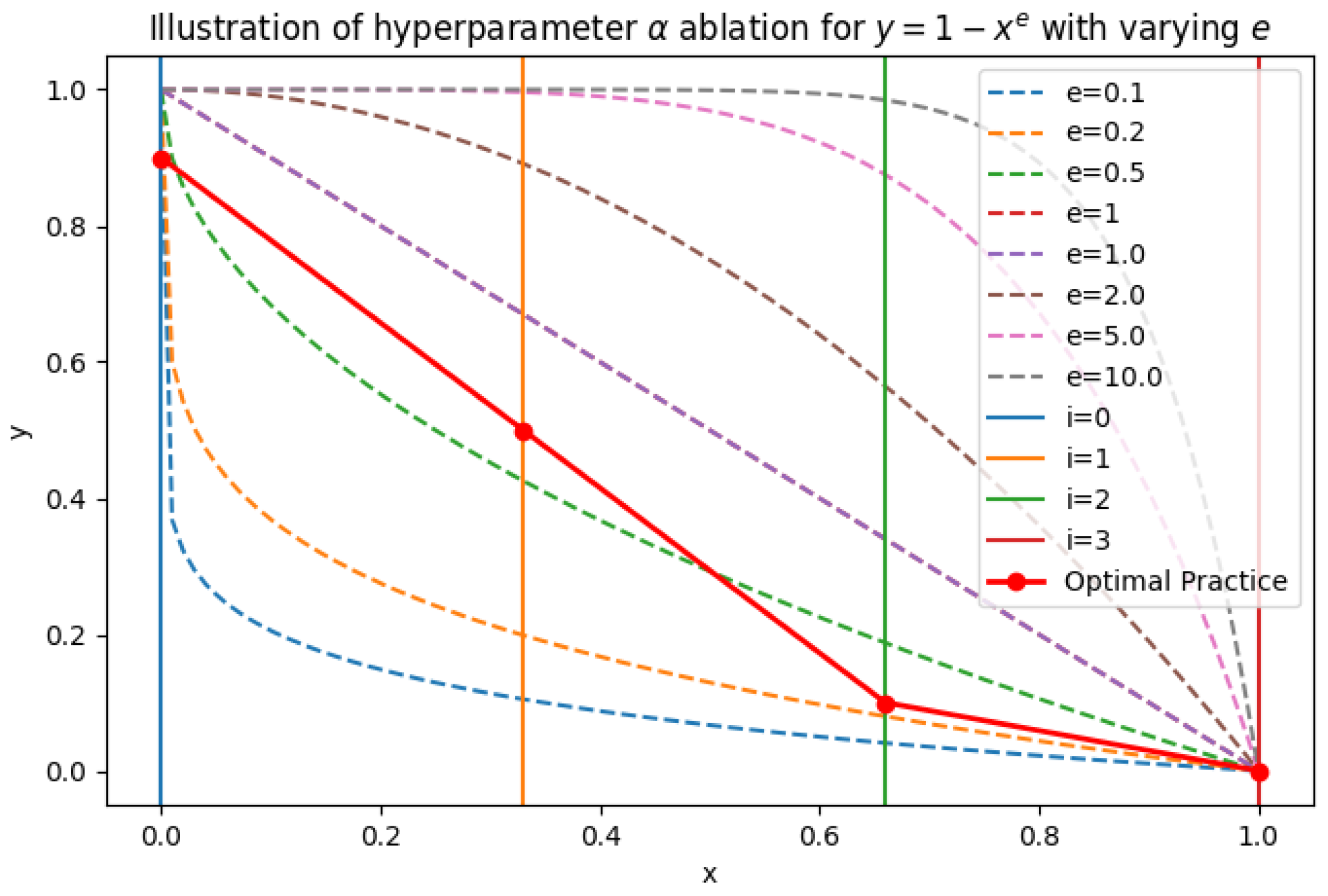
Analysis of α . The exponential curve family equation y = 1 x e has been selected to represent the changing pattern of the hyperparameter α . This hyperparameter α comprises a set of parameters that control the importance of the linear classifier and the cosine classifier during the training process, as defined in Equation (31). The parameter e acts as a novel hyperparameter that influences the behavior of α at each phase. Initially, the value of α is initialized at 1 and gradually diminishes to 0 by the final phase. In the exponential equation, the variable i represents the ith phase, while N represents the total number of phases, currently set at N = 4 . A detailed explanation of α is presented below:
α = 1 ( i 1 N 1 ) e .
There are several exponential monotonic decline curves with e as the parameter to control downward trend of α . The value of e is a set, [0.1, 0.2, 0.5, 1.0, 2.0, 5.0, 10.0]. The specific variations for e are depicted in Figure 3, and, the experimental results are presented in Table 3.
As the parameter e approaches near zero, a significant degradation in performance is observed. Optimal results are achieved when e = 5 . When e approaches zero, the cosine classifier’s loss weight during training quickly exceeds that of the linear classifier. This rapid transition prevents the linear classifier branch from converging adequately. Consequently, the cosine classifier serves as a fine-tuning mechanism, requiring guidance from the linear classifier to reach a better starting point. This underscores the necessity of a multi-stage training process. In our implementation, we empirically divide α and the training process into four stages by Figure 3, defined as follows:
α = 0.9 if 0 < e p o c h T 1 0.5 if T 1 < e p o c h T 2 0.1 if T 2 < e p o c h T 3 0 else wise .
As indicated in Table 3, it can be concluded that the hyperparameter α is sensitive. For instance, the difference in Intersection over Union (IoU) between e = 0.1 and e = 10 is 0.3%. We performed extensive search experiments using a set of exponential curves for e, with the current optimal practice presented in Equation (23). During the initial training phase, enabling backpropagation through the cosine classifier gradient enhances generalization, with the best results observed at e = 1 . The solid red line in Figure 3 is our best practice for tuning hyperparameters.
In ablation experiments, we also examined the generalization ability of solutions obtained through our training framework for minority categories. In the ISPRS dataset, the car class is a minority category, accounting for less than 2% of the total pixels. As the value of e increases, especially at e = 5 , the Intersection over Union (IoU) metric for the car category improves by 1%. This indicates that the obtained solution improves generalization for minority categories. Simultaneously, we observed that the final solution does not diminish the generalization ability for the primary categories.
Analysis of β . To understand the impact of the hyperparameter β on the main loss function (28), a range of β values was investigated. The hyperparameter β represents the importance assigned to the gradient of the regularization term in achieving a balanced space. As shown in Table 4, the sensitivity of the β hyperparameter within the selected range was found to be minimal.
Visual analysis. We plotted the loss curves of the MMA, as shown in Figure 4. The loss curves indicate that the MMA loss reaches its minimum value within a short period, likely in 1 to 4 epochs. In training progress, if the β value is close to 0, we observe an increase in the loss of MMA. This upward trend suggests a worsening of imbalance. Based on these observations, we empirically choose 0.5 as the default value for our experimental hyperparameter.

5.4. Category-Wise LID Dynamics Under Symmetric Noise Levels

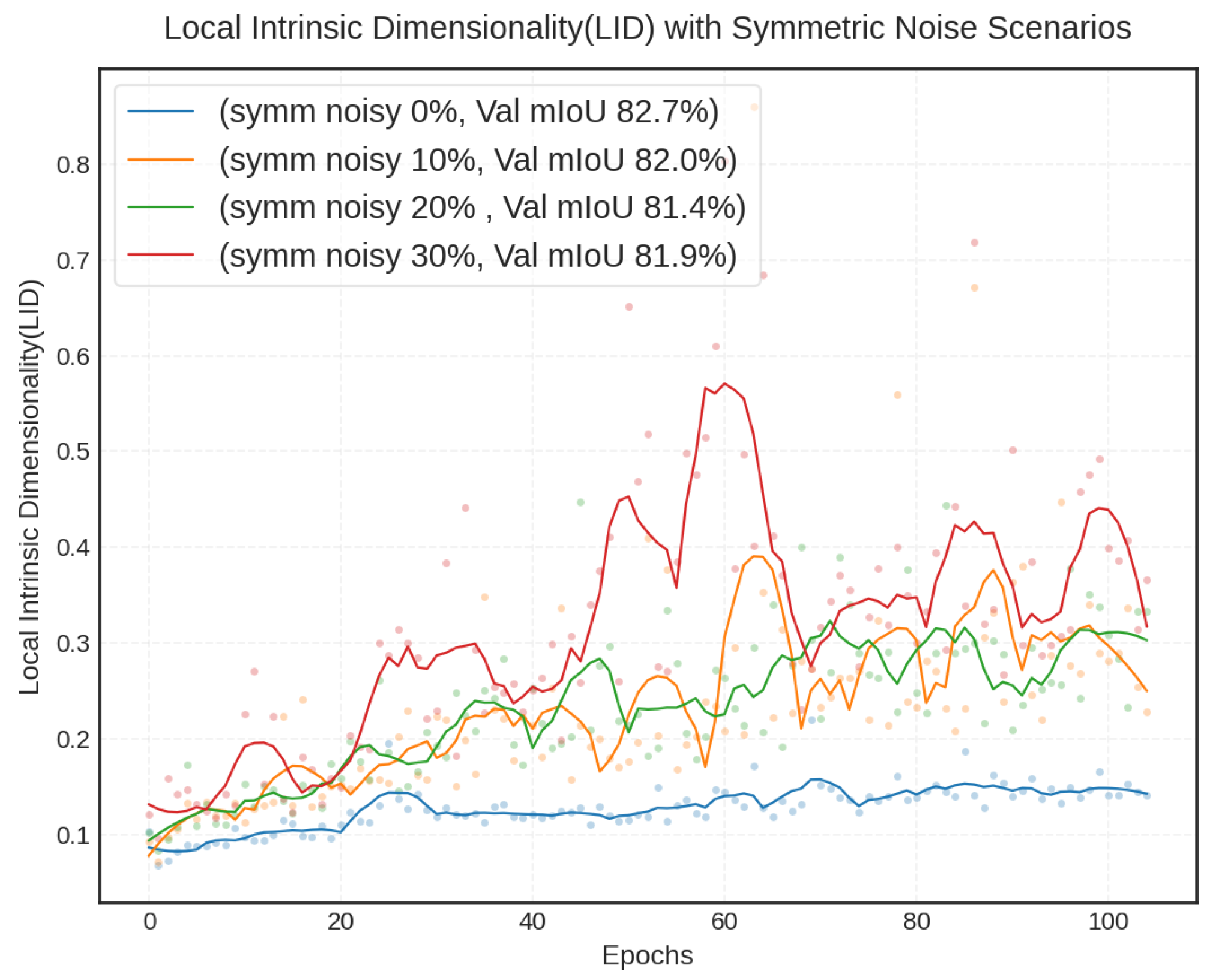
To further examine the stability of LID-based signals under varying annotation noise, we added symmetric noise to the training set of Vaihingen to simulate a synthetic noisy environment. A symmetric noisy environment may not match the noise patterns in real-world remote sensing data; it represents a controllable noise pattern. Figure 5 visualizes how the mean category-wise LID evolves throughout training across different symmetric noise levels. As the noise ratio increases, the overall category-wise Local Intrinsic Dimensionality (LID) values rise accordingly, indicating that noisier datasets induce more complex and ambiguous local data structures in representation. More importantly, the characteristic mid-training local maximum consistently appears across all noise settings, typically emerging around epochs 60 to 80, which shows that this peak is not an artifact of the origin data but a robust phenomenon.
Based on the joint analysis of Local Intrinsic Dimensionality (LID) and mean Intersection over Union (mIoU), we observe that the remote-sensing semantic segmentation model exhibits strong robustness to label noise, which forms the basis for the validity of our method. This indicates that the teacher model can still provide clean supervisory signals. Under 10% symmetric noise, the model achieves 82.0% accuracy, only a 0.7% drop compared with the noise-free setting, which achieves 82.7%. The accuracy is 81.4% under 20% symmetric noise and 81.9% under 30% symmetric noise. These results align with the measured category-wise LID trends, where LID increases with higher noise levels, suggesting that the model learns representations similar to those obtained in the clean condition. It means that pixels remain clustered into the correct semantic categories. The LID behavior observed under synthetic noise further supports the possibility that the original dataset contains mislabeled samples.
To validate the effectiveness of OPAB-stage1 under varying levels of label noise, we conducted experiments on the Vaihingen dataset with different symmetric noise intensities. As shown in Table 5, OPAB-stage1 consistently outperforms the baseline in OA, mIoU, and mF1 across all noise levels, demonstrating strong robustness against performance degradation. The method also achieves higher calibration accuracy on both training and test sets, indicating more reliable confidence estimates. Importantly, although symmetric noise patterns do not fully reflect real-world label corruption, the observed improvements still provide relative evidence that OPAB-stage1 effectively mitigates noisy-label effects and maintains stable semantic segmentation performance.

5.5. Loss Curves Analysis

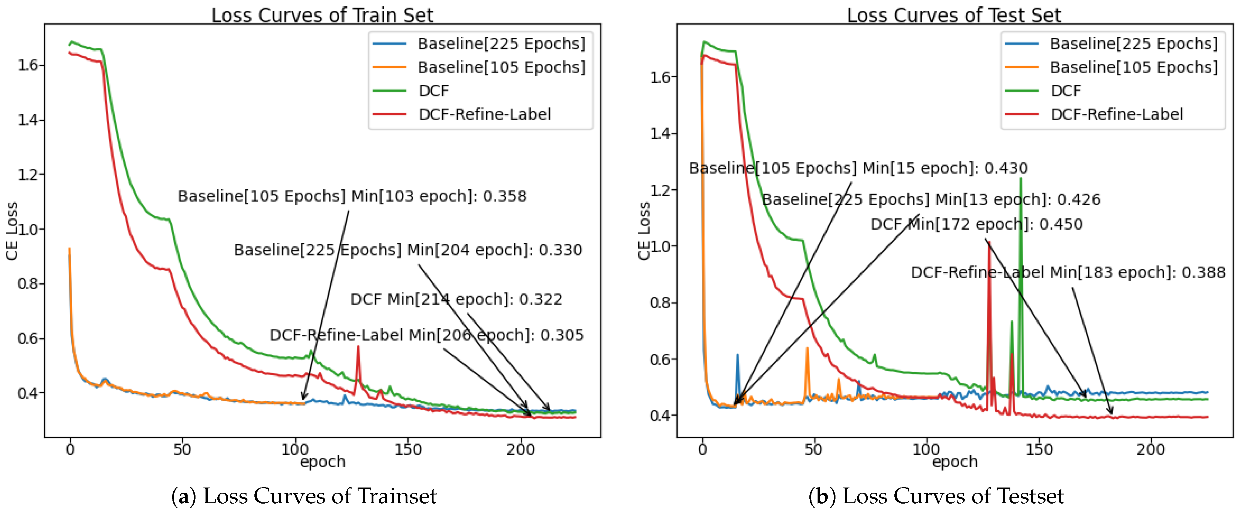
In order to enhance our comprehension of the OPAB training framework and active label calibration, we present the loss curves obtained during the training process, as illustrated in Figure 6. The standard training approach attains a minimal loss value prematurely on the test dataset. Conversely, the cosine classifier with MMA exhibits a lower training loss, suggesting an enhanced ability to fit the training data. Moreover, the calibrated dataset displays decreased loss values during both training and testing phases. A calibrated dataset that manifests reduced loss across both training and test datasets signifies a reduction in noise within the dataset as a whole. Introducing random alterations to the labels assigned to the training and test datasets is more likely to lead to higher loss values on the test dataset.

5.6. T-SNE Visualization

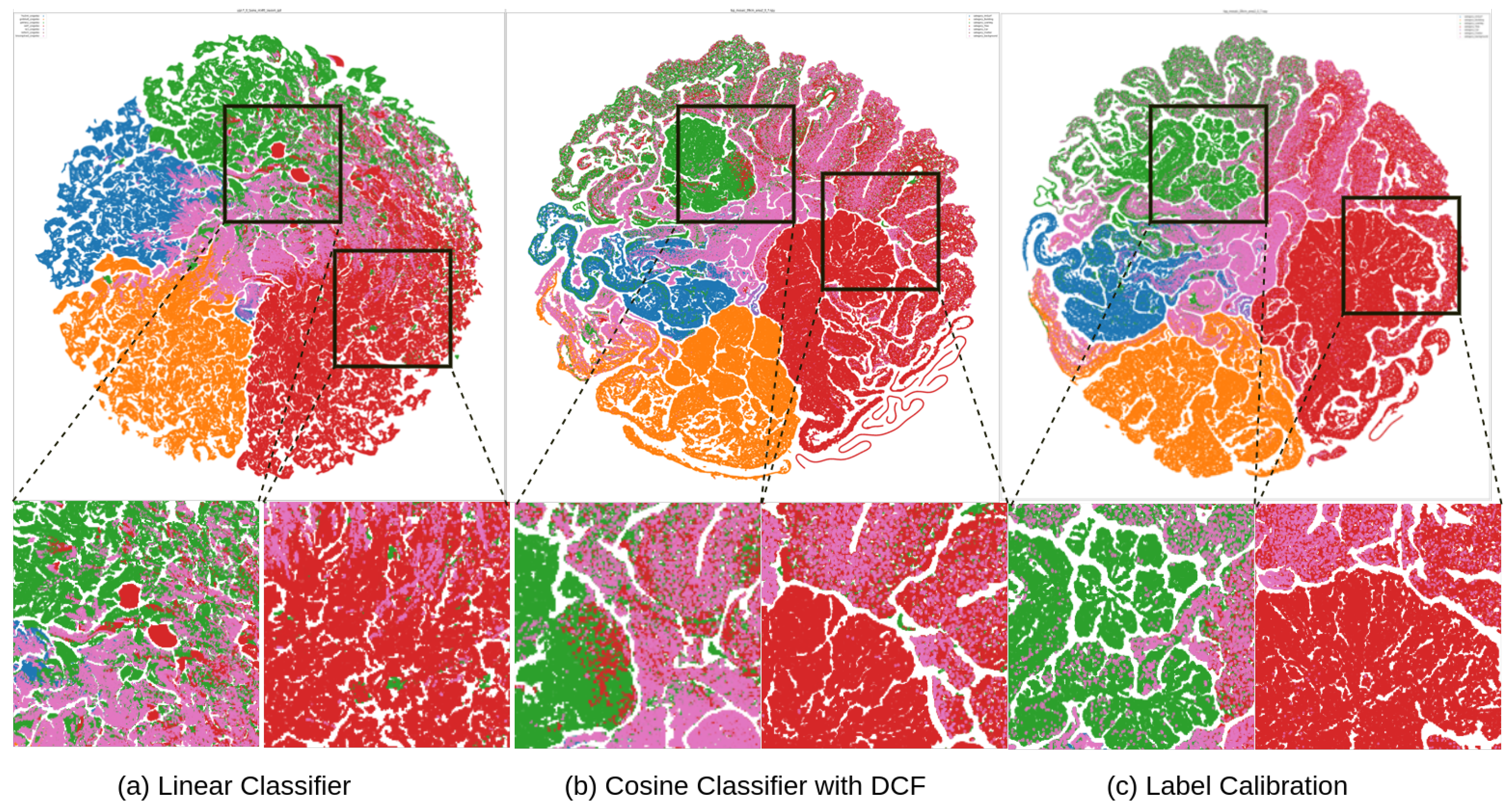
The t-SNE visualization presented in Figure 7 showcases the embedding space, where individual pixels are represented as points. The focus of the analysis is on the red and green regions, which correspond to the tree and low vegetation categories subject to label calibration. Examination of the plot reveals instances of sample overlap within regions associated with trees and low vegetation, suggesting potential mislabeling issues. A comparison between the outcomes of our OPAB training framework and a baseline training method, as illustrated in Figure 7, demonstrates that our approach enhances intra-class aggregation, leading to a higher density of class representation points. Furthermore, a decrease in overlap is observed for the tree and low vegetation categories following label calibration. In conclusion, the t-SNE plot provides additional evidence supporting the efficacy of our methodology.

5.7. Results on Comparative on Cross-Method Comparison Under Non-Ideal Annotation

To further evaluate the effectiveness of OPAB-stage1 under non-ideal annotations, we conducted a cross-method comparison with several representative strategies. These methods can be grouped into three categories: (1) loss function-based robust approaches, including GCE [67], SCE [30], and Focal [68], all evaluated using their default hyperparameters; (2) overfitting mitigation techniques, such as teacher-student distillation using an EMA strategy similar to that in AIO 2 [40], and loss control methods, Flooding [69], with a bias of 0.5 set based on observed training loss to prevent overfitting; (3) data augmentation-based strategies, exemplified by Mixup [55], where up to 50% of the training data was used to generate mixed samples.
All experiments were performed using the default parameters of each method, serving as a reference for comparative trends rather than rigorous hyperparameter optimization. As reported in Table 6, OPAB-stage1 achieves competitive or superior performance across multiple metrics, including mean F1 (mF1), mIoU, and overall accuracy (OA). These results demonstrate the robustness and effectiveness of OPAB-stage1 in handling non-ideal annotations for remote sensing image segmentation.

5.8. Results on (Online) Iteratively Calibration

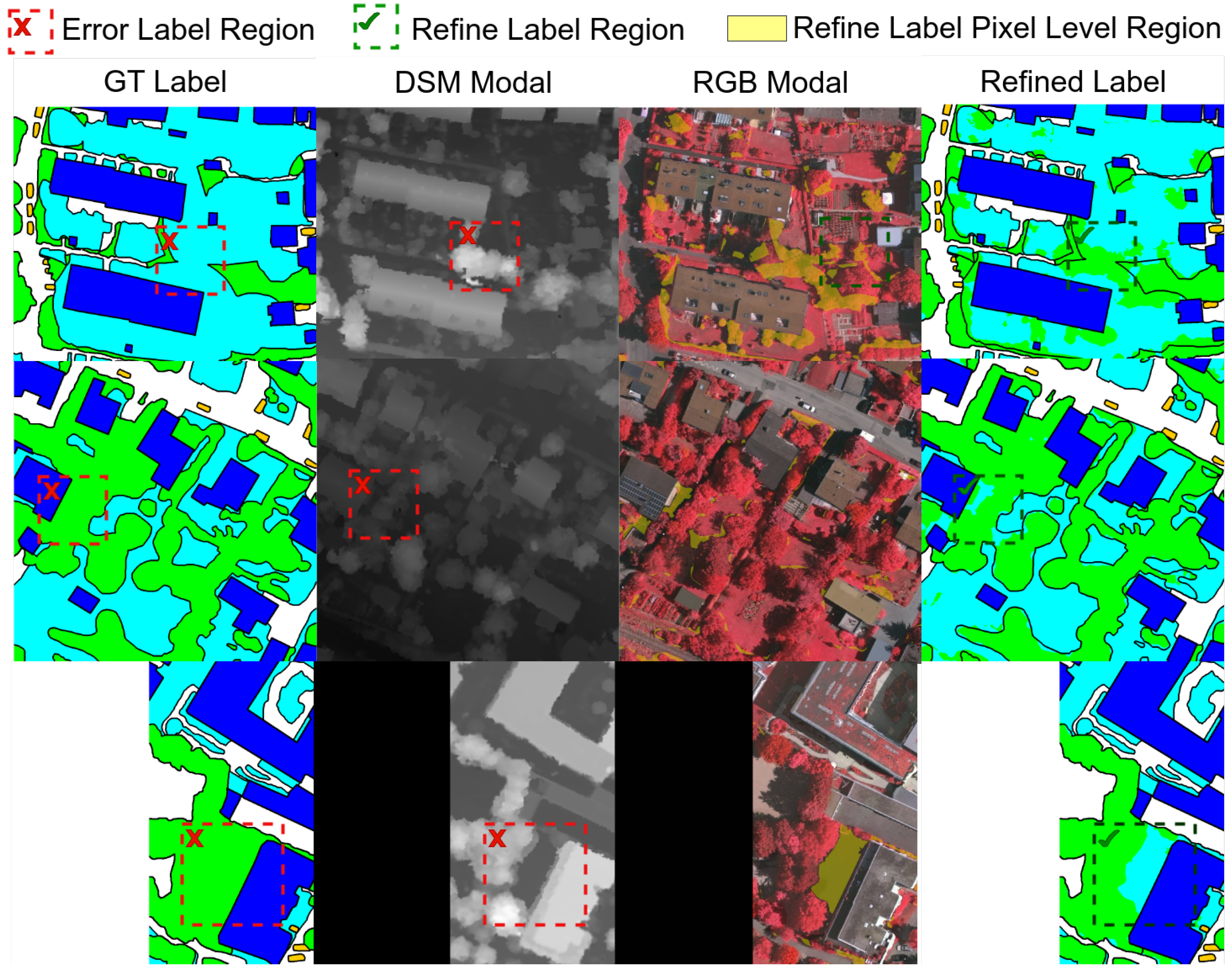
This section presents experiments on calibration between low vegetation and tree categories, using two baselines to evaluate the proposed algorithm’s efficacy; visualization of the corrections is shown in Figure 8. We compared the proposed calibration method between the original training process and our OPAB training process.
The results of multiple iterative experiments indicate that the pixel-level refinement process in Online Prototype Angular Balanced Self-Distillation (OPAB) converges. To evaluate the effectiveness of the active calibration program, we conducted several rounds of calibration. The calibration algorithm, as detailed in Table 7, modified approximately 5% of all labels, maintaining a consistent proportion across different calibration iterations. The results indicate that achieving balance in the embedding space has significant advantages, particularly for categories with lower levels of label noise. The synergy between structured embedding space and precise labeling enhances their efficacy, thereby significantly improving overall performance. Based on our findings, we recommend setting the default number of iterations to 3–5 cycles. Alternatively, calibration iterations can be terminated when successive calibrated labels exhibit minimal changes compared to the previous cycle. Moreover, the iterative calibration process also reflects the robustness of our algorithm. When label changes become negligible during iterations, it shows the algorithm has stabilized and confirms its reliability.

6. Discussion

6.1. Computational Complexity and Overhead Analysis

We evaluate the computational overhead of OPAB with respect to architectural complexity, training time, and calibration cost. First, OPAB introduces a lightweight BBN module by adding only a single linear layer to the classification head. This modification is negligible compared with the computational footprint of large backbones such as UNetformer, and thus does not materially increase per-iteration cost.
Second, the BBN strategy leads to a substantial increase in training time, typically by a factor of 2×. For UNetformer, each epoch requires approximately 10 s on the Vaihingen dataset and 60 s on the Potsdam dataset when trained on 2×Tesla V100 GPUs. With OPAB enabled, the total GPU-hours rise from 0.3 to 0.6 on Vaihingen and from 0.75 to 1.75 on Potsdam. On 1×Tesla T4, the overall training time is empirically observed to increase by roughly 6×. The primary source of this overhead is the extended training schedule imposed by BBN: the number of epochs increases from 105 to 225 for Vaihingen and from 45 to 105 for Potsdam, corresponding to an additional cycle of CosineAnnealingWarmRestarts scheduler.

6.2. Training Time and Efficiency Considerations

The computational overhead of the BBN module may exceed 2×; however, the BBN process can be removed if necessary. The goal of BBN is to construct balanced hyperspherical representations without degrading baseline performance. However, in real-world scenarios, we observed a performance degradation caused by directly replacing the classifier, as shown in Table 2. BBN is primarily designed to adapt to different baselines: setting α = 1 preserves baseline performance, while gradually decreasing α to 0 allows a smooth transition to a cosine classifier with MMA without performance loss. If replacing the final layer of the classifier with a cosine classifier directly under MMA achieves comparable performance, removing BBN can significantly reduce training time. As a compensatory measure, you can consider adjusting the hyperparameters using cyclic learning rate scheduling (CosineLRSchedule) in [17].
For the second stage of OPAB, fine-tuning can be performed without reinitialization or full training, thereby substantially reducing training time. The purpose of reinitializing the student model is to prevent the teacher model from learning poor solutions caused by noisy label data, which could hinder convergence to the optimal solution on clean data. Future improvements could consider geometric properties of the loss landscape, such as its connectivity. If the poor solutions induced by noisy labels lie within the gradient accumulation radius of the optimal solutions on clean data, direct fine-tuning is feasible. Understanding the linear connectivity among solutions from clean data can define the necessity of reinitialization. However, analysis of multi-model distance and connectivity in a loss landscape may be beyond the scope of this work and can be left for future study.
Regarding multi-round calibration, empirical results suggest that a single round is typically sufficient. Table 7 shows that most label corrections occur in the first round. If needed, an additional round can be performed to verify whether further pixel-level corrections are achieved, which can guide whether extra calibration is necessary.

6.3. Limitations and Future Work

Our OPAB framework advances semantic segmentation by tackling long-tail distributions and noisy labels, improving robustness and reducing angular deviation. However, it is limited by high computational cost and potential biases in label correction. Future work includes automating hyperparameter optimization and refining early stopping strategies. Although we intentionally selected a scenario with an unknown type of label noise, where noisy labels may exist in both the test and training sets, to validate our method’s applicability, it is still necessary to design a controllable noise scenario for validation. However, compared to classification tasks, designing a controllable, balanced, and noise-free dataset for semantic segmentation remains a challenge. Moreover, since clean datasets may remain consistently scarce and full manual calibration is highly resource-intensive, future work will also involve designing an appropriate human expert involvement mechanism to better assess the quality of modifications applied to non-ideal data in remote sensing semantic segmentation.

7. Conclusions

This study investigates labeling errors and class imbalance in semantic segmentation, proposing a strategy for their detection and correction. By integrating a balanced hypersphere representation, we enhance inter-class distances and improve noisy label classification. The method, embedded in a semi-supervised framework, mitigates label noise and boosts model performance in imbalanced settings. Its potential extends beyond remote sensing, especially in large-scale datasets with scarce data and sample imbalance, where tail samples are difficult to capture. As the complexity of semantic segmentation and image understanding tasks grows, addressing label noise and rare class samples becomes increasingly crucial. This approach offers broad applicability across diverse fields, such as medical imaging, autonomous driving, and video surveillance, promoting the development of universal image understanding systems and advancing AI technologies.

Supplementary Materials

The following supporting information can be downloaded at https://www.mdpi.com/article/10.3390/rs18010022/s1, Figure S1: Ideal Model for label errors detection; Figure S2 part I Illustration of calibration; Figure S2 part II Illustration of calibration.

Author Contributions

Conceptualization, H.L., H.M., H.Z., Y.L. and J.H.; methodology, H.L.; software, H.L.; validation, H.L. and Y.L.; formal analysis, H.M. and Y.L.; investigation, H.L., Y.L. and H.Z.; resources, H.M. and H.L.; data curation, H.M. and H.L.; writing—original draft preparation, H.L.; writing—review and editing, Y.L., H.M. and J.H.; visualization, H.L. and H.Z.; supervision, Y.L.; project administration, Y.L.; funding acquisition, Y.L. All authors have read and agreed to the published version of the manuscript.

Funding

This document is the result of the research project funded by the National Key Research and Development Plan under Grant 2021YFE0205700, the Science and Technology Development Fund of Macau project 0070/2020/AMJ, 00123/2022/A3, 0096/2023/RIA2, and the Zhuhai City Polytechnic Research Project (No. 2024KYBS02).

Institutional Review Board Statement

Not applicable.

Informed Consent Statement

Not applicable.

Data Availability Statement

The datasets are derived from the ISPRS Vaihingen and Potsdam datasets, with the links as follows: Vaihingen dataset: https://www.isprs.org/resources/datasets/benchmarks/UrbanSemLab/2d-sem-label-vaihingen.aspx accessed on 12 November 2025; Potsdam dataset: https://www.isprs.org/resources/datasets/benchmarks/UrbanSemLab/2d-sem-label-potsdam.aspx accessed on 12 November 2025.

Acknowledgments

We thank the open-source code of project UNetFormer for easy reproduction.

Conflicts of Interest

The authors declare that there is no conflicts of interest regarding the publication of this paper.

References

  1. Pacheco-Prado, D.; Bravo-López, E.; Martínez, E.; Ruiz, L.Á. Urban Tree Species Identification Based on Crown RGB Point Clouds Using Random Forest and PointNet. Remote Sens. 2025, 17, 1863. [Google Scholar] [CrossRef]
  2. Chen, Z.; Lin, Z.; Shi, T.; Deng, D.; Chen, Y.; Pan, X.; Chen, X.; Wu, T.; Lei, J.; Li, Y. Advancing Forest Inventory in Tropical Rainforests: A Multi-Source LiDAR Approach for Accurate 3D Tree Modeling and Volume Estimation. Remote Sens. 2025, 17, 3030. [Google Scholar] [CrossRef]
  3. Shi, L.; Zhang, X.; Halik, Ü. The Driving Mechanism and Spatio-Temporal Nonstationarity of Oasis Urban Green Landscape Pattern Changes in Urumqi. Remote Sens. 2025, 17, 3123. [Google Scholar] [CrossRef]
  4. Yilmaz, E.O.; Kavzoglu, T. DeepSwinLite: A Swin Transformer-Based Light Deep Learning Model for Building Extraction Using VHR Aerial Imagery. Remote Sens. 2025, 17, 3146. [Google Scholar] [CrossRef]
  5. García, G.; Antonio, J.; Lazzeri, G.; Tapete, D. Airborne and Spaceborne Hyperspectral Remote Sensing in Urban Areas: Methods, Applications, and Trends. Remote Sens. 2025, 17, 3126. [Google Scholar] [CrossRef]
  6. Kim, Y.; Yoon, D.; Kim, S.; Jeon, M. N Segment: Label-specific Deformations for Remote Sensing Image Segmentation. IEEE Geosci. Remote Sens. Lett. 2025, 22, 8003405. [Google Scholar] [CrossRef]
  7. Wei, J.; Sun, K.; Li, W.; Li, W.; Gao, S.; Miao, S.; Tan, Y.; Gui, W.; Duan, Y. Cross-Visual Style Change Detection for Remote Sensing Images via Representation Consistency Deep Supervised Learning. Remote Sens. 2025, 17, 798. [Google Scholar] [CrossRef]
  8. Zhang, W.; Shu, X.; Wu, S.; Ding, S. Semi-Supervised Change Detection with Data Augmentation and Adaptive Thresholding for High-Resolution Remote Sensing Images. Remote Sens. 2025, 17, 178. [Google Scholar] [CrossRef]
  9. Zhang, F.; Xia, K.; Yin, J.; Deng, S.; Feng, H. FFPNet: Fine-Grained Feature Perception Network for Semantic Change Detection on Bi-Temporal Remote Sensing Images. Remote Sens. 2024, 16, 4020. [Google Scholar] [CrossRef]
  10. Wang, L.; Zhang, M.; Gao, X.; Shi, W. Advances and challenges in deep learning-based change detection for remote sensing images: A review through various learning paradigms. Remote Sens. 2024, 16, 804. [Google Scholar] [CrossRef]
  11. Wang, Z.; Ding, Y.; Li, Y.; Wu, Z.; Yang, X.; Chen, Z. ACOC-MT: More Effective Handling of Real-World Noisy Labels in Remote Sensing Semantic Segmentation. IEEE Trans. Geosci. Remote Sens. 2025, 63, 4708318. [Google Scholar] [CrossRef]
  12. Sun, Y.; Liang, D.; Li, S.; Chen, S.; Huang, S.J. Handling noisy annotation for remote sensing semantic segmentation via boundary-aware knowledge distillation. IEEE Trans. Geosci. Remote Sens. 2025, 63, 4408720. [Google Scholar] [CrossRef]
  13. Qian, C.; Han, K.; Ding, J.; Lyu, C.; Yuan, Z.; Chen, J.; Liu, Z. Adaptive label correction for robust medical image segmentation with noisy labels. arXiv 2025, arXiv:2503.12218. [Google Scholar] [CrossRef]
  14. Li, R.; Zheng, S.; Zhang, C.; Duan, C.; Su, J.; Wang, L.; Atkinson, P.M. Multiattention network for semantic segmentation of fine-resolution remote sensing images. IEEE Trans. Geosci. Remote Sens. 2021, 60, 5607713. [Google Scholar] [CrossRef]
  15. Li, R.; Zheng, S.; Zhang, C.; Duan, C.; Wang, L.; Atkinson, P.M. ABCNet: Attentive bilateral contextual network for efficient semantic segmentation of fine-resolution remotely sensed imagery. ISPRS J. Photogramm. Remote Sens. 2021, 181, 84–98. [Google Scholar] [CrossRef]
  16. Wang, L.; Li, R.; Wang, D.; Duan, C.; Wang, T.; Meng, X. Transformer meets convolution: A bilateral awareness network for semantic segmentation of very fine resolution urban scene images. Remote Sens. 2021, 13, 3065. [Google Scholar] [CrossRef]
  17. Wang, L.; Li, R.; Zhang, C.; Fang, S.; Duan, C.; Meng, X.; Atkinson, P.M. UNetFormer: A UNet-like transformer for efficient semantic segmentation of remote sensing urban scene imagery. Isprs J. Photogramm. Remote Sens. 2022, 190, 196–214. [Google Scholar] [CrossRef]
  18. Wang, L.; Li, R.; Duan, C.; Zhang, C.; Meng, X.; Fang, S. A novel transformer based semantic segmentation scheme for fine-resolution remote sensing images. IEEE Geosci. Remote Sens. Lett. 2022, 3065, 6506105. [Google Scholar] [CrossRef]
  19. Hasan, A.; Saoud, L.S. Semantic labeling of high-resolution images using EfficientUNets and transformers. IEEE Trans. Geosci. Remote Sens. 2023, 61, 4402913. [Google Scholar]
  20. Li, Y.; Hou, Q.; Zheng, Z.; Cheng, M.M.; Yang, J.; Li, X. Large selective kernel network for remote sensing object detection. In Proceedings of the IEEE/CVF International Conference on Computer Vision, Paris, France, 1–6 October 2023. [Google Scholar]
  21. Tom, B.; Ravanbakhsh, M.; Demir, B. On the effects of different types of label noise in multi-label remote sensing image classification. IEEE Trans. Geosci. Remote Sens. 2022, 60, 1–13. [Google Scholar] [CrossRef]
  22. Liu, T.; Tao, D. Classification with noisy labels by importance reweighting. IEEE Trans. Pattern Anal. Mach. Intell. 2015, 38, 447–461. [Google Scholar] [CrossRef]
  23. Peng, Z.; Huang, W.; Guo, Z.; Zhang, X.; Jiao, J.; Ye, Q. Long-tailed distribution adaptation. In Proceedings of the 29th ACM International Conference on Multimedia, Virtual Event, China, 20–24 October 2021. [Google Scholar]
  24. Iliopoulos, F.; Kontonis, V.; Baykal, C.; Menghani, G.; Trinh, K.; Vee, E. Weighted distillation with unlabeled examples. Adv. Neural Inf. Process. Syst. 2022, 35, 7024–7037. [Google Scholar]
  25. Yi, K.; Wu, J. Probabilistic end-to-end noise correction for learning with noisy labels. In Proceedings of the IEEE/CVF Conference on Computer Vision and Pattern Recognition, Long Beach, CA, USA, 15–20 June 2019. [Google Scholar]
  26. Zheng, G.; Awadallah, A.H.; Dumais, S. Meta label correction for noisy label learning. In Proceedings of the AAAI Conference on Artificial Intelligence, Online, 2–9 February 2021; Volume 35. [Google Scholar]
  27. Sukhbaatar, S.; Bruna, J.; Paluri, M.; Bourdev, L.; Fergus, R. Training convolutional networks with noisy labels. arXiv 2014, arXiv:1406.2080. [Google Scholar]
  28. Ma, X.; Wang, Y.; Houle, M.E.; Zhou, S.; Erfani, S.; Xia, S.; Wijewickrema, S.; Bailey, J. Dimensionality-driven learning with noisy labels. In Proceedings of the International Conference on Machine Learning, PMLR, Stockholm, Sweden, 10–15 July 2018. [Google Scholar]
  29. Miao, Q.; Wu, X.; Xu, C.; Zuo, W.; Meng, Z. On better detecting and leveraging noisy samples for learning with severe label noise. Pattern Recognit. 2023, 136, 109210. [Google Scholar] [CrossRef]
  30. Wang, Y.; Ma, X.; Chen, Z.; Luo, Y.; Yi, J.; Bailey, J. Symmetric cross entropy for robust learning with noisy labels. In Proceedings of the IEEE/CVF International Conference on Computer Vision, Seoul, Republic of Korea, 27 October–2 November 2019. [Google Scholar]
  31. Reed, S.; Lee, H.; Anguelov, D.; Szegedy, C.; Erhan, D.; Rabinovich, A. Training deep neural networks on noisy labels with bootstrapping. arXiv 2014, arXiv:1412.6596. [Google Scholar]
  32. Han, B.; Yao, Q.; Yu, X.; Niu, G.; Xu, M.; Hu, W.; Tsang, I.; Sugiyama, M. Co-teaching: Robust training of deep neural networks with extremely noisy labels. Adv. Neural Inf. Process. Syst. 2018, 31, 1–11. [Google Scholar]
  33. Xie, J.; Li, Y.; Yang, S.; Li, X. Unsupervised Noise-Resistant Remote-Sensing Image Change Detection: A Self-Supervised Denoising Network-, FCM_SICM-, and EMD Metric-Based Approach. Remote Sens. 2024, 16, 3209. [Google Scholar] [CrossRef]
  34. Hossain, M.I.; Akhter, S.; Hong, C.S.; Huh, E.N. Single teacher, multiple perspectives: Teacher knowledge augmentation for enhanced knowledge distillation. In Proceedings of the Thirteenth International Conference on Learning Representations, Singapore, 24–28 April 2025. [Google Scholar]
  35. Liu, Y.; Wu, Z.; Lu, Z.; Nie, C.; Wen, G.; Zhu, Y.; Zhu, X. Noisy node classification by bi-level optimization based multi-teacher distillation. In Proceedings of the AAAI Conference on Artificial Intelligence, Philadelphia, PA, USA, 25 February–4 March 2025; Volume 39. [Google Scholar]
  36. Kaito, T.; Takahashi, T.; Sakata, A. The effect of optimal self-distillation in noisy gaussian mixture model. arXiv 2025, arXiv:2501.16226. [Google Scholar] [CrossRef]
  37. Bai, Y.; Yang, E.; Han, B.; Yang, Y.; Li, J.; Mao, Y.; Niu, G.; Liu, T. Understanding and improving early stopping for learning with noisy labels. Adv. Neural Inf. Process. Syst. 2021, 34, 24392–24403. [Google Scholar]
  38. Wang, X.; Wu, Z.; Lian, L.; Yu, S.X. Debiased learning from naturally imbalanced pseudo-labels. In Proceedings of the IEEE/CVF Conference on Computer Vision and Pattern Recognition, New Orleans, LA, USA, 18–24 June 2022. [Google Scholar]
  39. Prechelt, L. Early stopping-but when? In Neural Networks: Tricks of the Trade; Springer: Berlin/Heidelberg, Germany, 2002; pp. 55–69. [Google Scholar]
  40. Liu, C.; Albrecht, C.M.; Wang, Y.; Li, Q.; Zhu, X.X. AIO2: Online correction of object labels for deep learning with incomplete annotation in remote sensing image segmentation. IEEE Trans. Geosci. Remote Sens. 2024, 62, 5613917. [Google Scholar] [CrossRef]
  41. Bin, H.; Xie, Y.; Xu, C. Learning with noisy labels via clean aware sharpness aware minimization. Sci. Rep. 2022, 15, 1350. [Google Scholar]
  42. Lin, R.; Liu, W.; Liu, Z.; Feng, C.; Yu, Z.; Rehg, J.M.; Xiong, L.; Song, L. Regularizing neural networks via minimizing hyperspherical energy. In Proceedings of the IEEE/CVF Conference on Computer Vision and Pattern Recognition, Seattle, WA, USA, 13–19 June 2020. [Google Scholar]
  43. Kang, B.; Li, Y.; Xie, S.; Yuan, Z.; Feng, J. Exploring balanced feature spaces for representation learning. In Proceedings of the International Conference on Learning Representations, Vienna, Austria, 4 May 2021. [Google Scholar]
  44. Natarajan, N.; Dhillon, I.S.; Ravikumar, P.K.; Tewari, A. Learning with noisy labels. Adv. Neural Inf. Process. Syst. 2013, 26. [Google Scholar] [CrossRef]
  45. Zhou, B.; Cui, Q.; Wei, X.S.; Chen, Z.M. Bbn: Bilateral-branch network with cumulative learning for long-tailed visual recognition. In Proceedings of the IEEE/CVF Conference on Computer Vision and Pattern Recognition, Seattle, WA, USA, 13–19 June 2020. [Google Scholar]
  46. Wang, Z.; Xiang, C.; Zou, W.; Xu, C. Mma regularization: Decorrelating weights of neural networks by maximizing the minimal angles. Adv. Neural Inf. Process. Syst. 2020, 33, 19099–19110. [Google Scholar]
  47. Amsaleg, L.; Chelly, O.; Furon, T.; Girard, S.; Houle, M.E.; Kawarabayashi, K.I.; Nett, M. Estimating local intrinsic dimensionality. In Proceedings of the 21th ACM SIGKDD International Conference on Knowledge Discovery and Data Mining, Sydney, NSW, Australia, 10–13 August 2015. [Google Scholar]
  48. Shi, J.X.; Wei, T.; Xiang, Y.; Li, Y.F. How re-sampling helps for long-tail learning? Adv. Neural Inf. Process. Syst. 2023, 36, 75669–75687. [Google Scholar]
  49. Zhang, Z.; Feng, Z.; Yang, S. Semi-supervised object detection framework with object first mixup for remote sensing images. In Proceedings of the 2021 IEEE International Geoscience and Remote Sensing Symposium IGARSS, Brussels, Belgium, 11–16 July 2021. [Google Scholar]
  50. Hao, X.; Liu, L.; Yang, R.; Yin, L.; Zhang, L.; Li, X. A review of data augmentation methods of remote sensing image target recognition. Remote Sens. 2023, 15, 827. [Google Scholar] [CrossRef]
  51. Jiang, L.; Zhou, Z.; Leung, T.; Li, L.J.; Li, F.F. Mentornet: Learning data-driven curriculum for very deep neural networks on corrupted labels. In Proceedings of the International Conference on Machine Learning, PMLR, Stockholm, Sweden, 10–15 July 2018. [Google Scholar]
  52. Wei, J.; Liu, H.; Liu, T.; Niu, G.; Sugiyama, M.; Liu, Y. To smooth or not? when label smoothing meets noisy labels. arXiv 2021, arXiv:2106.04149. [Google Scholar]
  53. Lukasik, M.; Bhojanapalli, S.; Menon, A.; Kumar, S. Does label smoothing mitigate label noise? In Proceedings of the International Conference on Machine Learning, PMLR, Virtual, 13–18 July 2020. [Google Scholar]
  54. Ryota, H.; Yoshida, S.; Muneyasu, M. Confidentmix: Confidence-guided mixup for learning with noisy labels. IEEE Access 2024, 12, 58519–58531. [Google Scholar]
  55. Zhang, H.; Cisse, M.; Dauphin, Y.N.; Lopez-Paz, D. Mixup: Beyond empirical risk minimization. arXiv 2017, arXiv:1710.09412. [Google Scholar]
  56. Feng, Y.; Sun, X.; Diao, W.; Li, J.; Gao, X. Double similarity distillation for semantic image segmentation. IEEE Trans. Image Process. 2021, 30, 5363–5376. [Google Scholar] [CrossRef] [PubMed]
  57. Li, Y.; Yang, J.; Song, Y.; Cao, L.; Luo, J.; Li, L.J. Learning from noisy labels with distillation. In Proceedings of the IEEE International Conference on Computer Vision, Venice, Italy, 22–29 October 2017. [Google Scholar]
  58. Yi, R.; Huang, Y.; Guan, Q.; Pu, M.; Zhang, R. Learning from pixel-level label noise: A new perspective for semi-supervised semantic segmentation. IEEE Trans. Image Process. 2021, 31, 623–635. [Google Scholar] [CrossRef]
  59. Arazo, E.; Ortego, D.; Albert, P.; O’Connor, N.; McGuinness, K. Unsupervised label noise modeling and loss correction. In Proceedings of the International Conference on Machine Learning, PMLR, Long Beach, CA, USA, 9–15 June 2019. [Google Scholar]
  60. Huang, Y.; Bai, B.; Zhao, S.; Bai, K.; Wang, F. Uncertainty-aware learning against label noise on imbalanced datasets. In Proceedings of the AAAI Conference on Artificial Intelligence, Online, 22 February–1 March 2022; Volume 36. [Google Scholar]
  61. Li, Z.; Yang, X.; Meng, D.; Cao, X. An adaptive noisy label-correction method based on selective loss for hyperspectral image-classification problem. Remote Sens. 2024, 16, 2499. [Google Scholar] [CrossRef]
  62. Chen, J.; Ramanathan, V.; Xu, T.; Martel, A.L. Detecting Noisy Labels with Repeated Cross-Validations. In Proceedings of the International Conference on Medical Image Computing and Computer-Assisted Intervention, Marrakesh, Morocco, 6–10 October 2024; Springer: Cham, Switzerland, 2024. [Google Scholar]
  63. Ilya, L.; Hutter, F. Decoupled weight decay regularization. arXiv 2017, arXiv:1711.05101. [Google Scholar]
  64. Zhang, M.; Lucas, J.; Ba, J.; Hinton, G.E. Lookahead optimizer: K steps forward, 1 step back. Adv. Neural Inf. Process. Syst. 2019, 32. [Google Scholar]
  65. Olaf, R.; Fischer, P.; Brox, T. U-net: Convolutional networks for biomedical image segmentation. In Proceedings of the International Conference on Medical Image Computing and Computer-Assisted Intervention, Munich, Germany, 5–9 October 2015; Springer: Cham, Switzerland, 2015. [Google Scholar]
  66. Takumi, K. T-vMF similarity for regularizing intra-class feature distribution. In Proceedings of the IEEE/CVF Conference on Computer Vision and Pattern Recognition, Nashville, TN, USA, 20–25 June 2021. [Google Scholar]
  67. Zhang, Z.; Sabuncu, M. Generalized cross entropy loss for training deep neural networks with noisy labels. Adv. Neural Inf. Process. Syst. 2018, 31. [Google Scholar]
  68. Lin, T.Y.; Goyal, P.; Girshick, R.; He, K.; Dollár, P. Focal loss for dense object detection. In Proceedings of the IEEE International Conference on Computer Vision, Venice, Italy, 22–29 October 2017. [Google Scholar]
  69. Ishida, T.; Yamane, I.; Sakai, T.; Niu, G.; Sugiyama, M. Do we need zero training loss after achieving zero training error? arXiv 2020, arXiv:2002.08709. [Google Scholar]
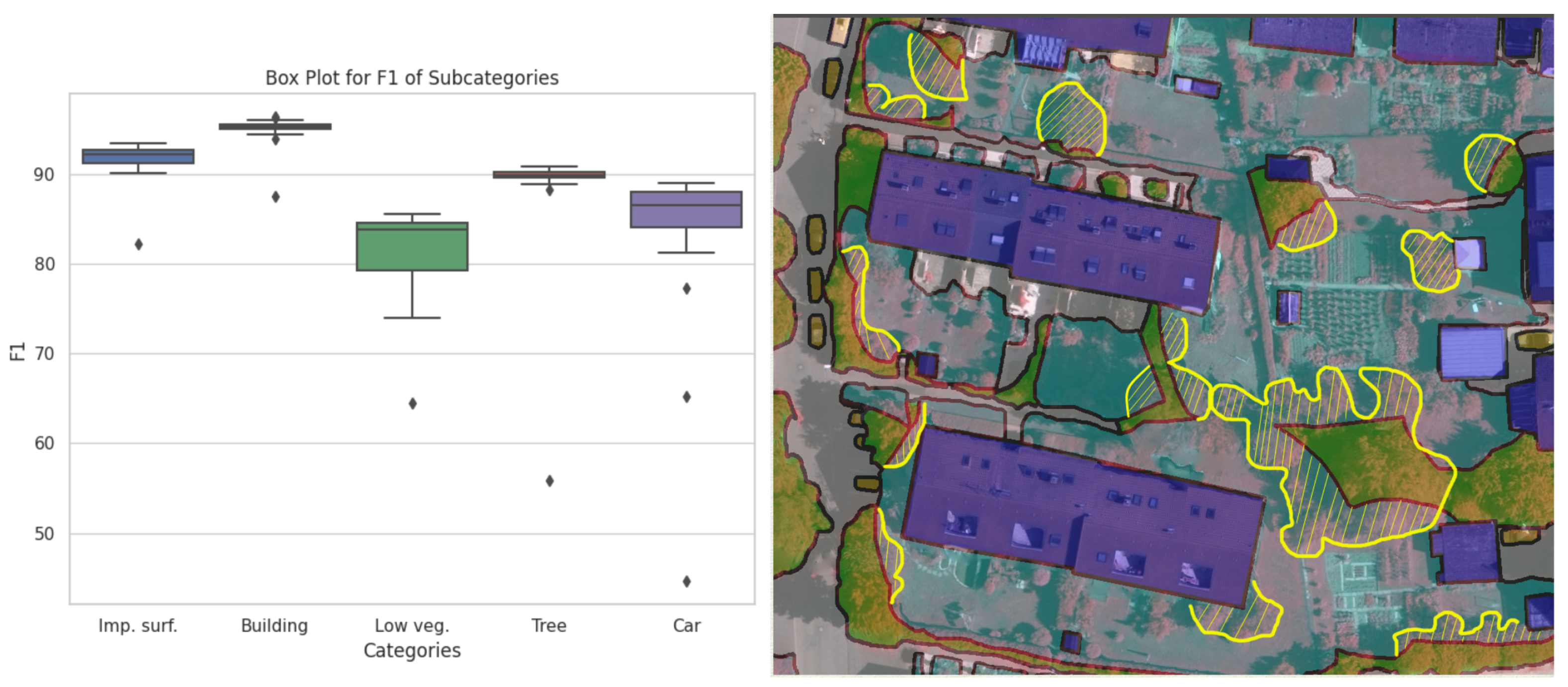
Figure 1. Performance analysis. The left figure shows box plots of performance for 20 backbones from survey papers [14,15,16,17,18,19,20] in ISPRS datasets. The yellow hatched area indicates regions that may contain errors, as identified through manual inspection. The mislabeled examples reveal that (1) low vegetation consistently underperforms with high variance; (2) trees and low vegetation are frequently confused, especially in manually corrected areas; and (3) labeling errors can cause performance issues even for visually clear vegetation regions [21]. This implies that, in real-world application datasets, there may be instances of non-ideal data, and model performance can be degraded by such non-ideal data.
Remotesensing 18 00022 g001
Figure 2. Online Prototype Angular Balanced Self-Distillation Framework (OPAB). Our method introduces a two-stage training strategy [45] to build a balanced hypersphere representation for both teacher and student models, improving label distribution and identifying mislabeled pixels. For label correction, we replace loss-based early stopping with LID to detect noisy labels and warm-up timing. We refine labels via a bootstrapping method guided by teacher predictions. We are using multi-round correction to handle unknown noise and improve model robustness.
Remotesensing 18 00022 g002
Figure 3. Illustration of simulation on the change trend of hyperparameter α . α = 1 ( i 1 N 1 ) e . The x-axis represents the training process progression. The dotted line section represents the exponential decay process. The exponential function is used to test different decay rates for α in the early and late stages. Using the exponential function can smoothly simulate the gradual decay in both stages. Detailed experimental results are shown in Table 3, indicating that the best results are achieved between e = 5 and e = 1 . By using the exponential function to further reduce the search interval, additional manual adjustments can yield even better results, as detailed in Figure 3.
Remotesensing 18 00022 g003
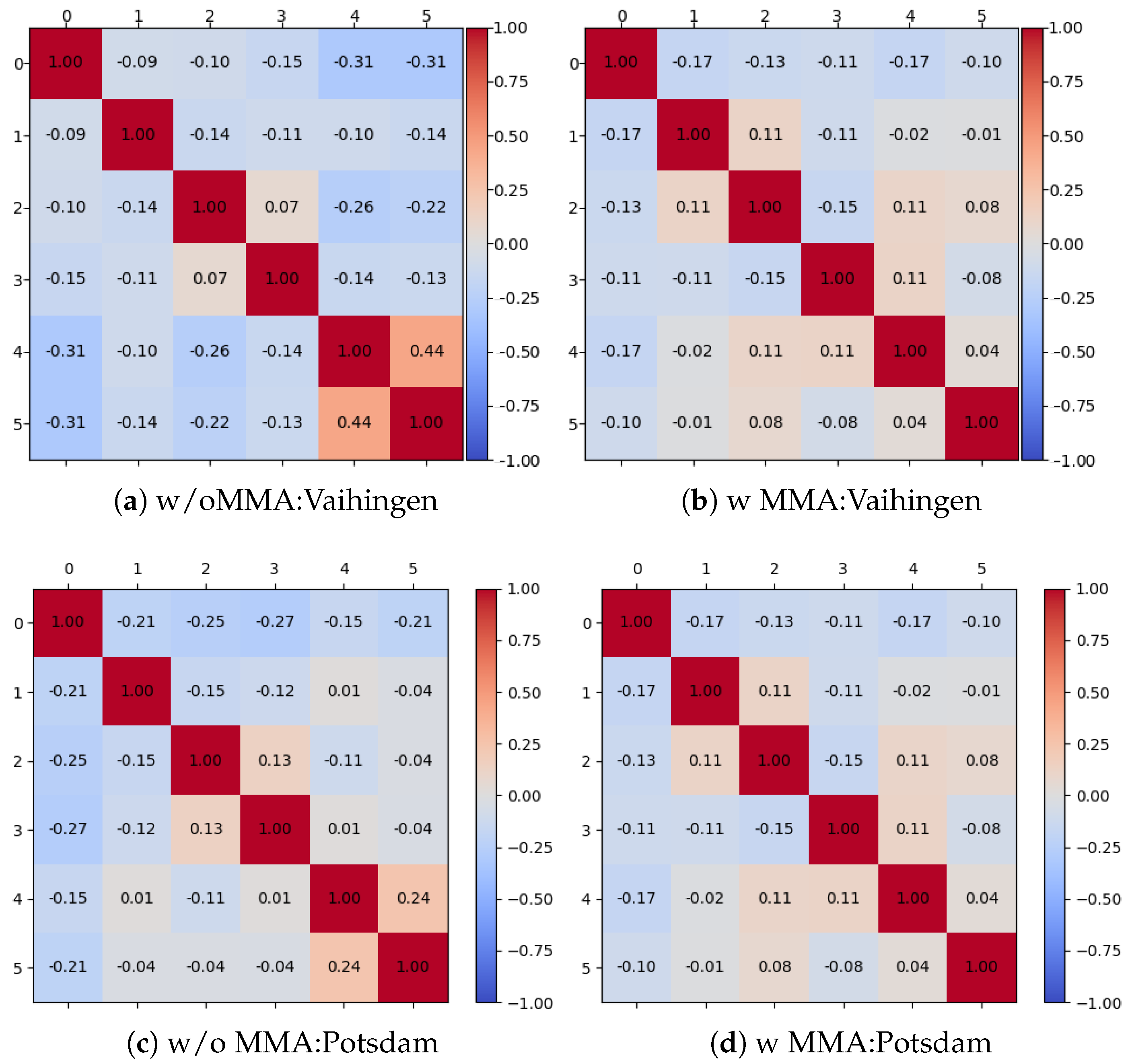
Figure 4. Illustration of the relationship between weight vectors from different channels on the last layer. The difference in angles between each of two channels tends to be minimal. The numbers in the grid denote the cosine values of the angles between class prototypes. Compared with (a), the inter-class prototype cosine differences in (b) are smaller, and similarly, those in (d) are smaller than in (c), indicating that MMA encourages the angles between class prototypes to become more uniform.
Remotesensing 18 00022 g004
Figure 5. Evolution of category-wise Local Intrinsic Dimensionality (LID) across training epochs under four symmetric noise settings of the origin Vaihingen training set (0%, 10%, 20%, 30%). As the noise ratio increases, the overall LID values rise accordingly, yet model performance declines only marginally, with a maximum drop of 1.3% mIoU. This suggests that the model retains strong robustness and can still learn representations similar to those acquired in noise-free environments even under elevated noise levels. The colored dots denote the actual measured LID values, with the line showing the corresponding smoothed trend.
Remotesensing 18 00022 g005
Figure 6. Illustration of loss curve analysis. OPAB minimizes the loss in training and testing in the last stage. The baseline training process achieves the minimum value earlier. The calibrated dataset has lower training and testing losses. DCF is the abbreviation of “Dual Classifier Framework” in bilateral-branch network (BBN).
Remotesensing 18 00022 g006
Figure 7. Illustration of the T-SNE plot for analysis of the embedding space. red is Tree, and green is Low Vegetation. The Dual Classifier Framework (OPAB) improves intra-class cohesion by calibrating mislabeled samples. As shown in (a), the linear classifier’s latent space contains inter-class noise, while the cosine classifier in (b) produces more compact and discriminative embeddings. After calibration (c), mislabeled samples are effectively removed, demonstrating OPAB’s capability in label error detection.
Remotesensing 18 00022 g007
Figure 8. Illustration of calibration, zoom in to observe details. Figure including the original GT, adjusted GT, corrected region’s RGB image, and DSM image. The yellow area in the RGB image indicates the region where labels were corrected, and the DSM image helps readers assess the effectiveness of the correction. More examples can be found in Supplementary Section S3.
Remotesensing 18 00022 g008
Table 1. Main results on Vaihingen and Potsdam datasets. Bold values denote the best results per backbone on each dataset.
BackboneTrainingDatasetVaihingenPotsdam
OA (%)mIoU (%)mF1 (%)OA (%)mIoU (%)mF1 (%)
UNet [65]Default [17]Original92.180.989.291.484.489.9
OPAB-stage192.181.189.391.784.990.2
Distillation [57]Refine92.681.389.491.988.293.7
OPAB (ours)93.984.691.593.988.792.7
BANet [16]Default [17]Original90.581.489.691.086.392.5
OPAB-stage192.983.290.691.586.692.7
Distillation [57]Refine93.785.191.892.789.194.2
OPAB (ours)94.786.892.893.089.594.4
DC-Swin [18]Default [17]Original91.683.289.892.087.593.2
OPAB-stage193.484.691.591.987.293.0
Distillation [57]Refine94.685.291.893.390.094.7
OPAB (ours)95.187.893.493.490.294.8
UNetformer [17]Default [17]Original91.082.790.492.886.891.3
OPAB-stage193.584.791.592.887.091.6
Distillation [57]Refine94.285.492.093.189.794.5
OPAB (ours)95.789.094.193.789.994.6
Table 2. Mean F1 (mF1), overall accuracy and mIoU of UNetformer on Vaihingen and Potsdam. The cosine classifier Impaired the generalization ability. OPAB as fine-tuning leads to better results on both cases. -> represents direction of fine-tuning in BBN framework.
Vaihingen-F1 (%) Metrics
MethodsClassifier>Imp.surfBuildingLowvegTreeCarOA (%)mIoU (%)mF1 (%)
baseline [17]linear92.795.384.990.688.59182.790.4
MMA [46]linear96.995.884.789.987.893.483.991.0
BBN [45]linear->linear96.695.384.489.987.99383.690.8
BBN w MMAlinear->linear96.895.584.790.188.593.283.891.0
cosine [66]cosine96.195.584.290.050.092.674.483.2
cosine w MMAcosine96.695.584.790.278.493.181.089.1
OPAB w/o MMAlinear->cosine97.095.885.090.188.793.584.391.3
OPAB (ours)linear->cosine96.995.685.490.389.493.584.791.5
Potsdam-F1 (%) Metrics
MethodsClassifierImp.surfBuildingLowvegTreeCarOA (%)mIoU (%)mF1 (%)
baseline [17]linear93.697.287.788.996.592.886.591.3
MMA [46]linear93.796.387.589.196.292.686.591.5
BBN [45]linear->linear93.795.987.089.296.592.586.291.1
BBN w MMAlinear->linear94.096.387.389.696.392.786.691.3
cosine [66]cosine93.996.287.689.095.992.586.391.3
cosine w MMAcosine94.096.387.589.196.292.686.591.3
OPAB w/o MMAlinear->cosine93.996.387.589.396.592.786.691.4
OPAB (ours)linear->cosine94.296.687.689.396.592.887.091.6
Table 3. Mean F1 (mF1), overall accuracy and mIoU of α analysis. Opt.Prac. is the abbreviation of optimal practice.
VaihingenF1 (%)Metrics
e Imp. Surf. Building Low Tree Car OA (%) mIoU (%) mF1 (%)
0.196.895.784.790.188.693.384.191.2
0.296.895.484.690.388.693.384.191.2
0.596.995.784.690.189.093.484.391.3
196.995.684.690.289.493.384.491.3
296.895.484.790.189.393.384.291.2
596.995.584.690.189.593.384.491.3
1096.995.684.690.289.493.384.491.3
Opt. Prac.96.995.685.490.389.493.584.791.5
Table 4. Mean F1 (mF1), overall accuracy and mIoU of β analysis.
VaihingenF1 (%)Metrics
Beta Imp.Surf. Building Low Tree Car OA (%) mIoU (%) mF1 (%)
0.196.995.584.790.28993.484.391.3
0.396.995.584.990.388.793.484.391.3
0.596.995.784.990.188.793.484.391.3
0.796.995.784.890.188.893.484.391.3
0.996.995.684.790.189.293.484.491.3
Table 5. Performance comparison under different levels of symmetric label noise on the Vaihingen dataset. Validation metrics include OA, mIoU, and mF1, while calibration accuracy is reported on both training and test sets.
Val-Set Metrics (%)Calibration Accuracy (%)
Noise (%)Method OA mIoUmF1 Train Set Test Set
0baseline [17]91.082.790.4
OPAB-stage193.584.794.1
10baseline [17]90.882.089.888.986.3
OPAB-stage193.584.191.290.487.0
20baseline [17]90.681.489.589.086.1
OPAB-stage193.484.091.190.186.9
30Baseline [17]90.781.989.889.086.2
OPAB-stage193.584.191.290.386.9
Table 6. MeanF1 (mF1), overall accuracy and mIoU of cross-method comparison.
Backbone Vaihingen Potsdam
UnetFormer OA (%) mIoU (%) mF1 (%) OA (%) mIoU (%) mF1 (%)
baseline [17]91.082.790.492.886.891.3
gce [67]93.283.590.892.285.790.7
sce [30]93.483.490.892.586.291.3
focal [68]93.383.790.992.285.891.0
ema [40]93.383.590.892.285.991.0
flooding [69]93.483.590.892.486.191.1
mixup [55]86.777.590.492.185.790.9
OPAB-stage193.584.791.592.887.091.6
Table 7. Per-class F1 scores (%) and metrics of active calibration loops on Vaihingen. r[number] is round index. origin means the setting in [17].
VaihingenF1 (%)MetricsTotal
Round Training Dataset Imp.Surf. Building Low Veg. Tree Car OA (%) mIoU (%) mF1 (%) Pixel Change
-originorigin92.795.384.990.688.591.082.790.4-
r[0]OPABorigin96.895.885.390.789.193.584.791.50.00% (+0.00%)
r[1]OPABby-r[0]96.995.792.096.889.195.789.094.14.12% (+4.12%)
r[2]OPABby-r[1]96.895.792.197.188.895.789.194.14.29% (+0.17%)
r[3]OPABby-r[2]96.995.792.697.288.995.889.394.24.29% (+0.00%)
r[4]OPABby-r[3]96.995.992.597.389.295.989.594.34.26% (−0.03%)
r[5]OPABby-r[4]96.995.792.697.389.095.889.494.34.26% (−0.00%)
r[6]OPABby-r[5]96.995.792.397.288.895.889.394.24.24% (−0.02%)
Disclaimer/Publisher’s Note: The statements, opinions and data contained in all publications are solely those of the individual author(s) and contributor(s) and not of MDPI and/or the editor(s). MDPI and/or the editor(s) disclaim responsibility for any injury to people or property resulting from any ideas, methods, instructions or products referred to in the content.