Article

Global–Local Mamba-Based Dual-Modality Fusion for Hyperspectral and LiDAR Data Classification

School of Computer Science, Northwestern Polytechnical University, Xi’an 710129, China
*
Author to whom correspondence should be addressed.
Remote Sens. 2026, 18(1), 138; https://doi.org/10.3390/rs18010138
Submission received: 24 November 2025 / Revised: 15 December 2025 / Accepted: 18 December 2025 / Published: 31 December 2025
(This article belongs to the Section AI Remote Sensing)

Highlights

What are the main findings?
  • We propose GL-Mamba, a frequency-aware dual-modality fusion network that combines low-/high-frequency decomposition, global–local Mamba blocks, and cross-attention to jointly exploit hyperspectral and LiDAR information for land-cover classification.
  • GL-Mamba achieves state-of-the-art performance on the Trento, Augsburg, and Houston2013 benchmarks, with overall accuracies of 99.71%, 94.58%, and 99.60%, respectively, while producing smoother and more coherent classification maps than recent CNN-, transformer-, and Mamba-based baselines.
What are the implications of the main findings?
  • The results demonstrate that linear-complexity Mamba state-space models are a competitive and efficient alternative to heavy transformer architectures for large-scale multimodal remote sensing, enabling accurate HSI–LiDAR fusion under practical computational constraints.
  • The proposed frequency-aware and cross-modal design can be extended to other sensor combinations and tasks (e.g., multispectral–LiDAR mapping, change detection), providing a general blueprint for building scalable and robust multimodal networks in remote sensing applications.

Abstract

Hyperspectral image (HSI) and light detection and ranging (LiDAR) data offer complementary spectral and structural information; however, the integration of these high-dimensional, heterogeneous modalities poses significant challenges. We propose a Global–Local Mamba dual-modality fusion framework (GL-Mamba) for HSI–LiDAR classification. Each sensor’s input is decomposed into low- and high-frequency sub-bands: lightweight 3D/2D CNNs process low-frequency spectral–spatial structures, while compact transformers handle high-frequency details. The outputs are aggregated using a global–local Mamba block, a state-space sequence model that retains local context while capturing long-range dependencies with linear complexity. A cross-attention module aligns spectral and elevation features, yielding a lightweight, efficient architecture that preserves fine textures and coarse structures. Experiments on Trento, Augsburg, and Houston2013 datasets show that GL-Mamba outperforms eight leading baselines in accuracy and kappa coefficient, while maintaining high inference speed due to its dual-frequency design. These results highlight the practicality and accuracy of our model for multimodal remote-sensing applications.

1. Introduction

Hyperspectral image (HSI) records hundreds of contiguous spectral bands and has become a core tool in remote sensing for fine-grained material analysis. Beyond land-cover classification, recent deep models have pushed HSI towards advanced tasks such as spectral unmixing, anomaly detection and change detection. For example, DGMNet adopts a dual-branch unmixing network that combines an adaptive graph-convolutional branch with a Mamba-based sequence modeller to recover accurate sub-pixel abundances in complex scenes [1]. In hyperspectral anomaly detection, memory-augmented autoencoders with adaptive reconstruction and sample-attribution mining explicitly model normal background behaviour so that rare targets can be isolated more robustly [2]. For change detection, interpretable low-rank sparse unmixing and spatial attention-enhanced difference mapping networks integrate physically motivated unmixing priors with deep feature learning to highlight subtle spectral changes over time [3]. However, HSI alone lacks explicit three-dimensional structural information. Light Detection and Ranging (LiDAR) provides complementary elevation and geometric cues, and recent multimodal approaches have shown that jointly modelling HSI spectra and LiDAR height information through cross-attention collaboration or adaptive feature alignment with Global–Local Mamba modules can significantly improve land-cover classification performance [4,5]. Motivated by these advances, this paper proposes a new Global–Local Mamba-based dual-modality fusion framework for hyperspectral and LiDAR data classification.
Amazing developments in remote sensing over the past few decades have improved our ability to observe and understand the Earth’s surface. The combination of light detection and ranging (LiDAR) with hyperspectral image (HSI) data represents a major breakthrough. HSIs contain rich spectral data across hundreds of narrow bands which can enhance the detection of small chemical, physical, and contextual properties that standard RGB images may miss. LiDAR provides high-resolution three-dimensional structural information. The fusion of both types of data allows for better inference than either one alone, but the differences in spatial resolution, data sampling densities by type, and noise have made achieving fusion difficult.
The early fusion literature concentrated on convolutional architectures and attention mechanisms to cohere spectral and geometric cues. For example, the Cross-Attention Bridge network used two cross-attention modules to disentangle spectral and structural information, which led to significantly improved classification performance [4]. Building off this idea, multiple researchers contributed to LiDAR-guided cross attention, which uses LiDAR signals to help choose the informative hyperspectral bands [6], and then HSLiNets, which have two nonlinear paths for efficient dual-modality fusion [7]. Other examples of early work include state-space models like MSFMamba which account for the long-range dependencies across modalities [8], adaptive gating and learnable transformers [9], dual branch transformers for separating spectral and elevation [10], feature-decision collaborative fusion networks [11], cross-modal semantic enhancement [12], coupled adversarial learning [13], graph based multimodal fusion [14], cross-attention multi-scale convolution networks [15], multi-scale graph encoder–decoder models [16], multiscale adaptive fusion [17], transformer based enhancement modules [18], and hypergraph convolution networks [19]. While the field may have moved on, particularly the introduction of transformer architectures and hybrid methods have allowed long-range dependencies and multimodal interactions to be reflected more robustly. For example, FusionFormer-X utilizes hierarchical top-down self-attention to be applied to multimodal scene understanding [20]. Multi-feature cross attention-induced transformers combine multiple streams of attention to support many features [21]. Hybrid fusion schemes that supported fusion of cue via feature-level and decision-level cues [22]. Recent approaches utilized meta-learning and prompt tuning to adapt a network with the stimulus of the scene [23], as well as using multiscale attention with modified transformers to independently reweight features at various scales [24]. It has also been possible to use reinforcement learning to learn the optimal fusion pathways [25], as well as unsupervised methods such as unified anchor graph learning that jointly clusters multiple features across modalities [26]. Finally, there were additional transformer-based innovations such as cross hyperspectral and LiDAR attention transformers [27], interactive transformer–CNN networks [28], local-to-global cross-modal attention-aware integration [29], graph-infused hybrid vision transformers [30], a comprehensive survey on the trends in hyperspectral image classification [31], multimodal transformer cascaded fusion nets [32], and deep fuzzy fusion networks [33].
The latest studies (2024–2025) develop additional improvements and new avenues. Heterogeneous Attention Feature Fusion Networks maintain modality-specific attention in different branches [34]. HyperPointFormer extends cross attention to 3D point clouds [35],and AFA-Mamba utilizes global–local Mamba blocks to facilitate adaptive feature alignment [5]. Mamba-based joint classification drives fusion using state-space models [36]. There are even developments in hierarchical fusion and separation with height information [37], and cross-modal hierarchical frequency fusion separates and fuses signals according to low- and high-frequency components [38]. This work illustrates that the development of multimodal remote sensing continues to build on cross attention, graph reasoning, adversarial learning, sequence modeling, reinforcement learning, and state-space models. Domain generalization is particularly important in remote sensing because models trained on one geographic region often suffer performance degradation when applied to different areas due to variations in sensor characteristics, atmospheric conditions, and land-cover distributions. Recent works have addressed this challenge through structural optimization and distribution-independent feature learning. Zhang et al. proposed a structural optimization transmission approach that uses optimal transport to align feature distributions across domains for HSI–LiDAR classification [39]. More recently, Gao et al. introduced a feature-distribution-independent network (FDINet) for multisource remote sensing cross-domain classification without explicit feature alignment [40]. These advances motivate the design of GL-Mamba, which implicitly promotes generalization through frequency-aware decomposition and linear-complexity state-space modeling that captures domain-invariant spectral–spatial patterns.
Despite these advancements, many challenges persist. Several of these models are computationally intense, and are not practical for real-time or edge applications, and it is not trivial to align spectral and geometric information across dimensions. Additionally, a performance penalty arises and careful design is required to keep the long-range dependencies in consideration while providing enough local context. Therefore, our work contributes to understanding these challenges by proposing a Global–Local Mamba-based dual-modality fusion framework (GL-Mamba) for hyperspectral and LiDAR data classification, by proposing what we discovered as the Global–Local Mamba-based dual modality with multiple frequency bands for fusion. The network proposed outputs HSI and LiDAR data in a low-frequency and high-frequency way, uses a combination of conventional 2D/3D CNNs to process the low- and high-frequency HSI data alongside lightweight transformers, combines the 2D HSI and 3D LiDAR data through the global–local Mamba block to maintain local contexts while modelling long-range dependencies, and extracts both spectral- and elevation-oriented features using cross-attention methods. In comparison to references on multiple benchmarks, we found our work achieves the highest accuracy while maintaining some computational efficiencies alongside, which re-affirms the potential for various combinations of these newest deep-learning paradigms.
This article’s main contributions are outlined below:
  • The Global–Local Mamba dual-modality fusion network is developed which uses a state-space Mamba block to learn both local spectral–spatial context as well as long-range dependencies from hyperspectral and LiDAR inputs with linear complexity.
  • A dual-branch frequency decomposition is introduced to decompose hyperspectral and LiDAR signals into low- and high-frequency components, with each component processed separately using lightweight 3D/2D CNNs and compact transformers, preserving fine detail and coarser structure while minimising computational costs.
  • Our approach has been rigorously tested on the Trento, Augsburg, and Houston2013 benchmarks with different patch sizes, proving its robustness and generalizability. When compared against eight state-of-the-art baselines, it always comes out on top in terms of kappa, average accuracy, and overall accuracy.
This work is organized as follows. Section 2 outlines the details of the proposed network; Section 3 provides the experimental data; Section 4 includes an ablation study; Section 5 concludes the article and addresses future work.

2. Materials and Methods

2.1. Preliminaries

Mathematically, let the hyperspectral image (HSI) be denoted by X H R H     W     B and the corresponding LiDAR raster by X L R H     W , where H and W are the spatial height and width, and B is the number of spectral bands after PCA. For each central pixel, we extract an S     S patch from both modalities and denote the i-th input pair as x ( i ) = ( x H ( i ) , x L ( i ) ) . The ground-truth label of the i-th sample is y true ( i ) { 1 , 2 , , C } , where C is the number of land-cover classes. The network outputs a probability vector y ^ ( i ) R 1     C , and is trained with cross-entropy loss. For quick reference, the main notations used in this paper are summarised in Table 1.

2.2. Overall Architecture

The overall architecture of the proposed GL-Mamba model is illustrated in Figure 1. The framework simultaneously exploits hyperspectral imaging (HSI) and LiDAR data through a frequency-aware dual-branch design. Hyperspectral images provide rich spectral signatures but suffer from limited spatial resolution, while LiDAR offers precise elevation and structural information. By decomposing each modality into low- and high-frequency components, the framework processes spectral and spatial features separately and then fuses them through a global–local Mamba module and a cross-attention bridge. We denote the input HSI cube as X H R H     W     B and the LiDAR raster as X L R H     W , where H and W are spatial dimensions and B is the number of spectral bands after principal component analysis (PCA).

2.3. Frequency-Aware Decomposition

For each modality, we separate low- and high-frequency components using a computationally efficient filtering strategy. Low-frequency bands contain smooth spectral/spatial variations that are well modelled by convolutional neural networks (CNNs), whereas high-frequency bands capture fine details suited to transformers.
Specifically, the low-frequency component is extracted using average pooling as a low-pass filter, and the high-frequency component is obtained by subtracting the smoothed signal from the original input:
X H low = AvgPool k     k ( X H ) ,
X H high = X H Upsample ( X H low ) ,
where k denotes the pooling kernel size (set to 3 in our experiments). This formulation provides a parameter-free, reproducible approach equivalent to a simple low-pass/high-pass filter pair. The same decomposition strategy is applied to the LiDAR raster to obtain X L low and X L high .
F H low = Conv 3 D int 8 ( X H low ) ,
where Conv 3 D int 8 denotes a 3D convolution with integer quantisation and X H low is the low-frequency HSI component. The high-frequency spectral component is encoded with a lightweight transformer operating in fp16 precision:
F H high = Transformer fp 16 ( X H high ) .
The concatenated HSI feature is
F H = Concat F H low , F H high .
Similarly, the LiDAR raster is split into low-frequency elevation data and high-frequency edge structures. Low-frequency spatial features are extracted using a depthwise separable 2D convolution operating in Int8:
F L low = DWConv int 8 ( X L low ) ,
while high-frequency features are captured with a transformer:
F L high = Transformer fp 16 ( X L high ) ,
and the resulting LiDAR embedding is
F L = Concat F L low , F L high .

2.4. Global–Local Mamba Fusion

After obtaining feature maps F H and F L , we iteratively fuse them through three stages using a structured state-space model (SSM) called Mamba. At each stage s, the fused input U s feeds into a global–local Mamba unit that captures long-range dependencies and local offsets. The architecture of the GL-Mamba fusion module is shown in Figure 2.
The SSM updates its hidden state h t for sequence position t as
h t = A ¯ h t 1 + B ¯ u t ,
where u t is the concatenated HSI–LiDAR token at position t and A ¯ , B ¯ are state matrices generated by exponentiating parameter increments. The output of the global channel is
y t = C h t + D u t ,
for learnable matrices C and D. A depthwise convolution implements a local channel DWConv ( u t ) . These two channels are blended by a sigmoid gate:
g t = σ W g [ y t ; DWConv ( u t ) ] ,
which produces the final fused token
u ˜ t = g t y t + ( 1 g t ) DWConv ( u t ) .
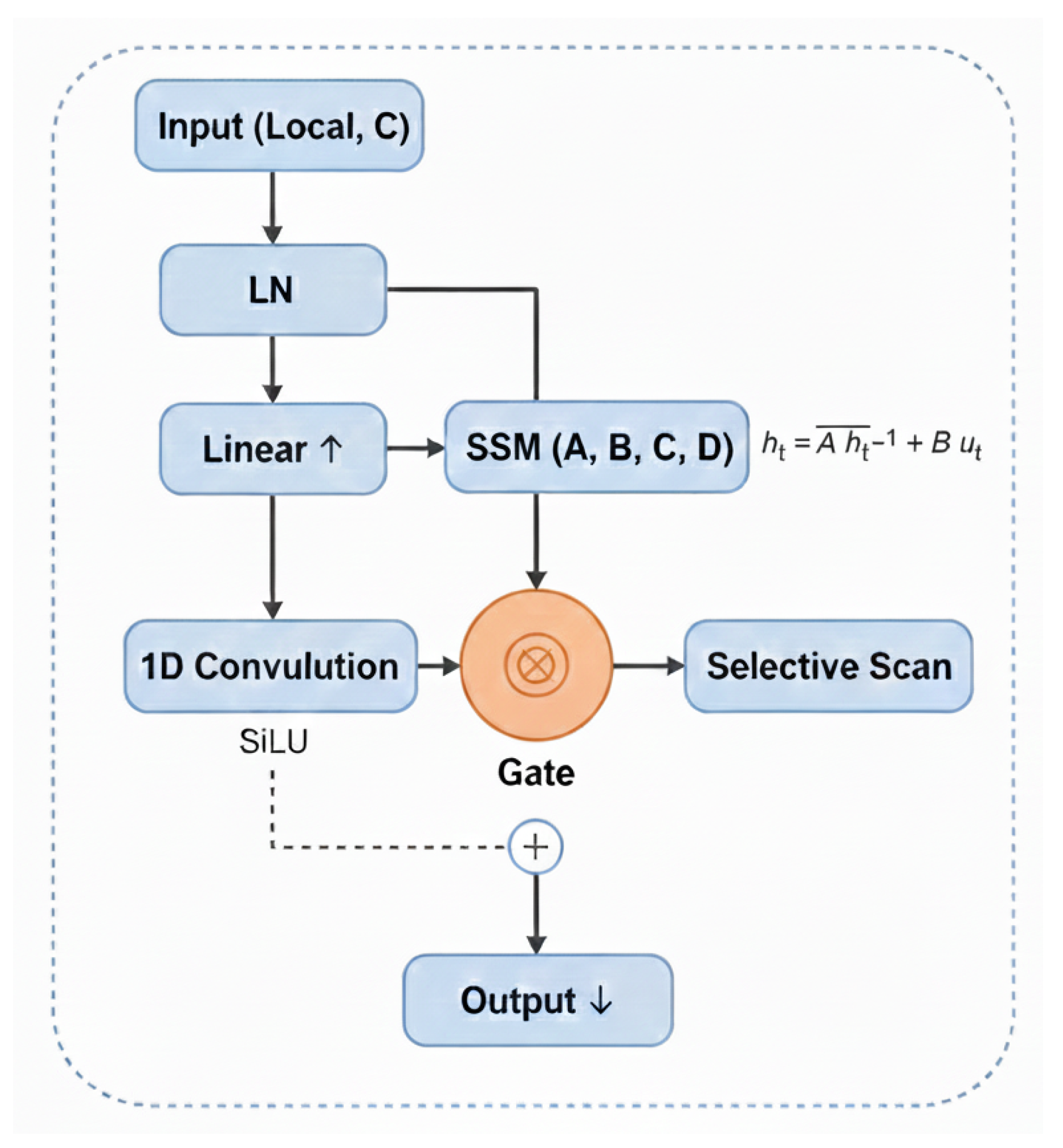
The adaptive fusion weights ( α , β , γ ) are computed dynamically based on the input features rather than being fixed parameters. As shown in Equation (14), W fusion is a learnable projection matrix that takes the concatenated feature representations from all three branches as input. The softmax function produces normalized weights that sum to unity. This design enables the network to adapt to varying scene content: for inputs where spectral information is more discriminative, the network assigns higher weights to α and β (HSI branches); for inputs where elevation cues are more important, γ (LiDAR branch) receives higher weight. The weights are computed per-sample, allowing instance-specific feature weighting during both training and inference. Detailed architecture of the Simplified Mamba Block is shown in Figure 3.
Across three branches (HSI low, HSI high, LiDAR), a shared Mamba kernel mixes features using learned scalar weights α , β , γ obtained via a softmax:
Z = α Mamba ( U ( 1 ) ) + β Mamba ( U ( 2 ) ) + γ Mamba ( U ( 3 ) ) ,
[ α , β , γ ] = Softmax W fusion [ U ( 1 ) ; U ( 2 ) ; U ( 3 ) ] .
A 1     1 convolution then predicts spatial offsets
Δ = Conv 1     1 ( Z ) , Z aligned = warp ( Z , Δ ) ,
which correct cross-modal misalignments at each stage. The aligned output feeds into the next stage: U s + 1 = Z aligned .

2.5. Cross-Attention Bridge

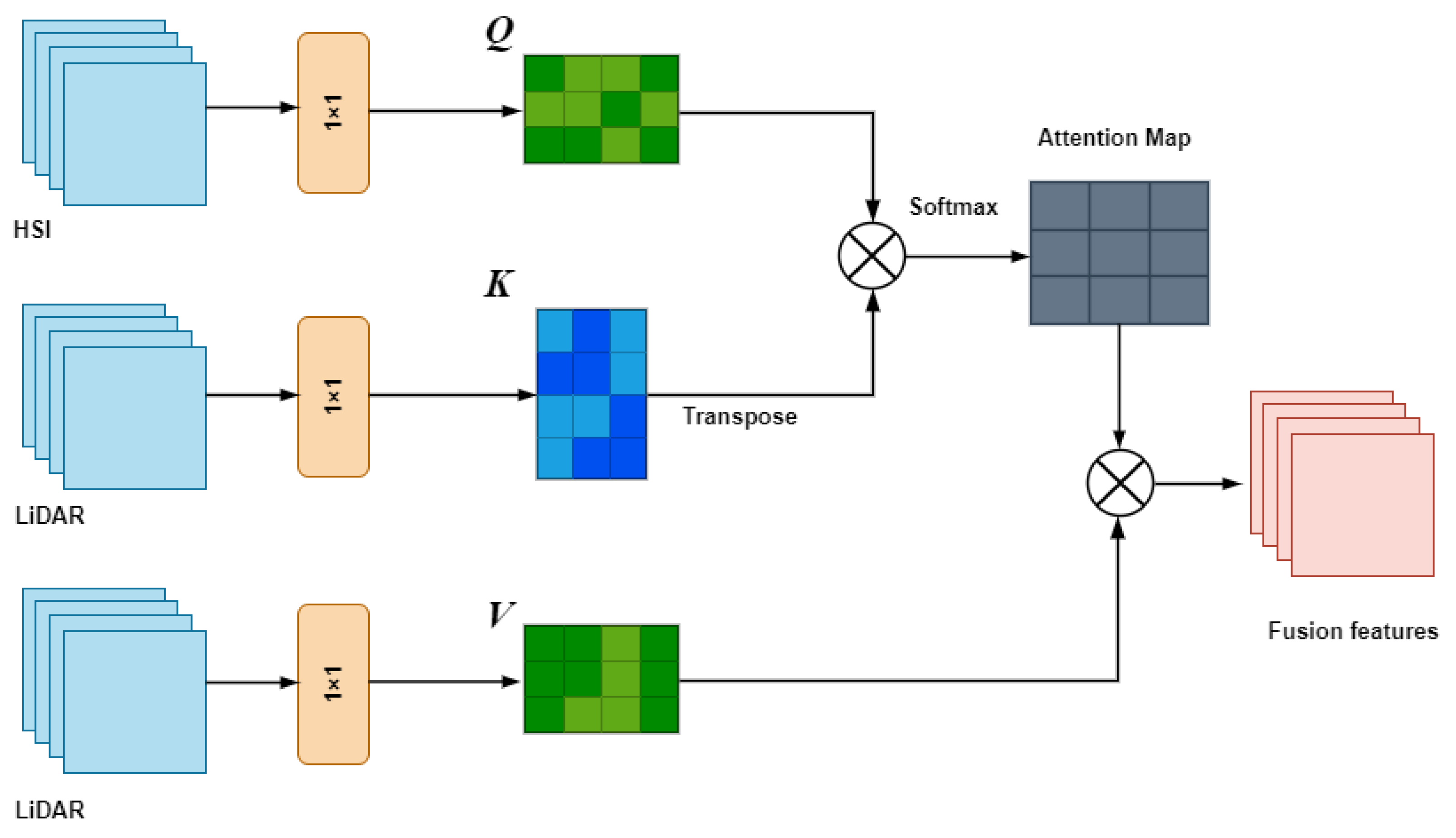
After three Mamba stages, we obtain final HSI and LiDAR tokens, denoted F H ( 3 ) and F L ( 3 ) . These features enter a cross-attention module (CAM), which allows HSI queries to attend to LiDAR keys and values, as illustrated in Figure 4. First, we flatten spatial dimensions to yield sequences of length N = H     W and linearly project them to queries, keys and values:
Q = F H ( 3 ) W Q , K = F L ( 3 ) W K , V = F L ( 3 ) W V .
The scaled dot-product attention is computed as
Attention ( Q , K , V ) = Softmax Q K d k V ,
where d k is the key dimension. Multi-head attention concatenates outputs from h heads and applies a final projection:
F fused = Concat Attention 1 , , Attention h W O .

2.6. Classification

Outputs from all three fusion stages are aggregated via element-wise addition:
F global = Z ( 1 ) + Z ( 2 ) + Z ( 3 ) .
A 1     1 convolution and global average pooling reduce spatial dimensions, and a fully connected layer produces class logits z . The final land-cover prediction is obtained with softmax activation:
y ^ = Softmax FC ( GAP ( Conv 1     1 ( F global ) ) .
Training minimizes the cross-entropy loss
L = i = 1 C y i log y ^ i ,
where y i is the one-hot label for class i. Optimization uses Adam and random data augmentation to improve robustness.

2.7. Algorithm

Algorithm 1 summarises the training and inference procedures.
Algorithm 1 GL-Mamba Classification Pipeline
Require: Hyperspectral image X H R H     W     B , LiDAR data X L R H     W
Ensure: Classified map Y ^
 1:
Preprocessing: Apply PCA on X H ; normalize X L
 2:
Patch Extraction: Divide into S     S patches; decompose into ( X H low , X H high , X L low , X L high )
 3:
HSI Feature Extraction:   F H low Conv 3 D ( X H low ) , F H high Transformer ( X H high )
 4:
LiDAR Feature Extraction:   F L low DWConv 2 D ( X L low ) , F L high Transformer ( X L high )
 5:
GL-Mamba Fusion: Fuse { F H low , F H high , F L low , F L high } via three-stage GL-Mamba blocks
 6:
Cross-Attention:   Q F H W Q , K F L W K , V F L W V ; F fused Softmax ( Q K / d k ) · V
 7:
Classification:   Y ^ Softmax ( FC ( GAP ( F fused ) ) )
 8:
return   Y ^

3. Results

Three public multimodal remote sensing image categorization datasets are implemented to evaluate the effectiveness of the proposed method: Houston2013, Trento, and Augsburg. The complete parameters are detailed in Table 2.

3.1. Configuration of Parameters

The proposed GL-Mamba model is trained using a range of patch and batch sizes over 200 epochs with cross-entropy loss. The PyTorch deep-learning framework and Python 3.10 are used for implementation. Experiments were conducted on a Windows 10 workstation equipped with an Intel Core i7-9th Gen CPU, 16 GB of RAM, and an NVIDIA GeForce GTX 1660 Ti GPU. For performance evaluation, three standard metrics are employed: overall accuracy (OA), average accuracy (AA), and the Kappa coefficient.

3.2. Comparison of Patch Size and OA Effects

The proposed method utilizes CNN as the backbone for the GL-Mamba component. The feature extraction ability of CNNs with transformer components varies considerably with input patch size. Figure 5 compares patch size and OA across all datasets.
The experimental results demonstrate that different patch sizes generate varying classification characteristics. In the Augsburg dataset, overall accuracy increases with patch size from 5     5 to 11     11 , with 11     11 being optimal. In Houston2013, overall accuracy increases from 5     5 to 9     9 ; however, at 11     11 , accuracy drops by approximately 15%, with peak performance at 9     9 . In Trento, overall accuracy peaks at 7     7 . These results indicate that optimal patch size should be determined according to the distinct characteristics of each dataset.

3.3. Comparison of Learning Rate on Datasets

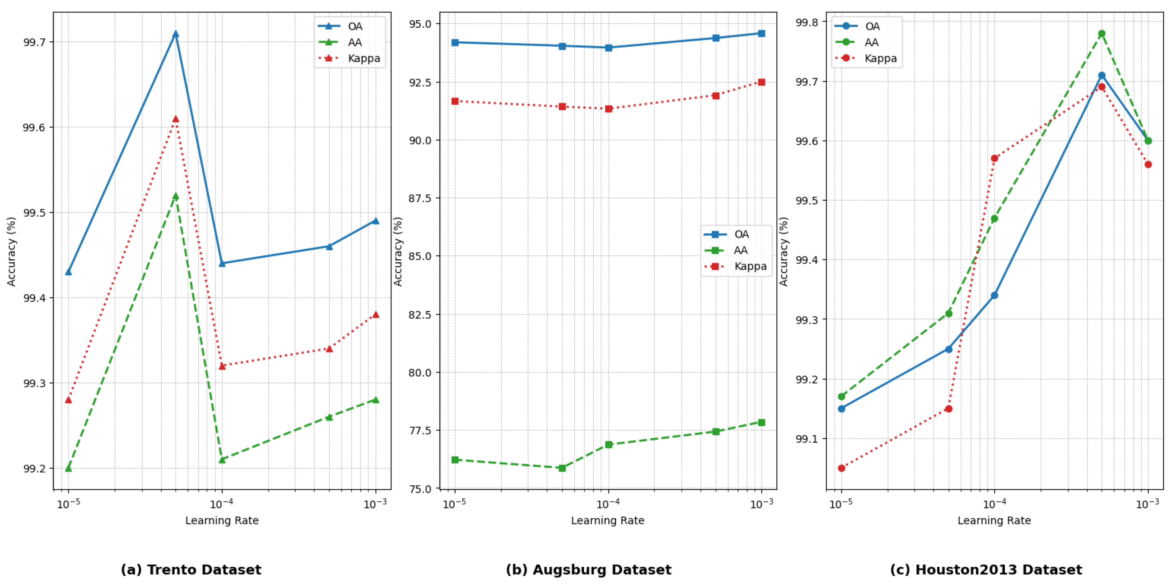
The learning rate is one of the most crucial hyperparameters in deep learning, controlling how the network weights are updated based on the loss gradient. An excessively high learning rate leads to unstable parameter updates and prevents convergence, while an excessively low learning rate may trap network parameters in local minima. Classification results were evaluated for learning rates ranging from 0.001 to 0.00001. The findings show that 0.00001 is optimal for all three datasets, as shown in Figure 6.

3.4. Comparison and Analysis of Classification Performance

We evaluated the proposed GL-Mamba model on three benchmark datasets against eight state-of-the-art baselines: CALC [13], CCR-Net [44], ExViT [45], DHViT [46], SAL2RN [47], MS2CANet [48], DSHF [49], and S3F2Net [50]. We evaluated class-specific accuracy and quantitatively presented OA, AA, and Kappa coefficient.
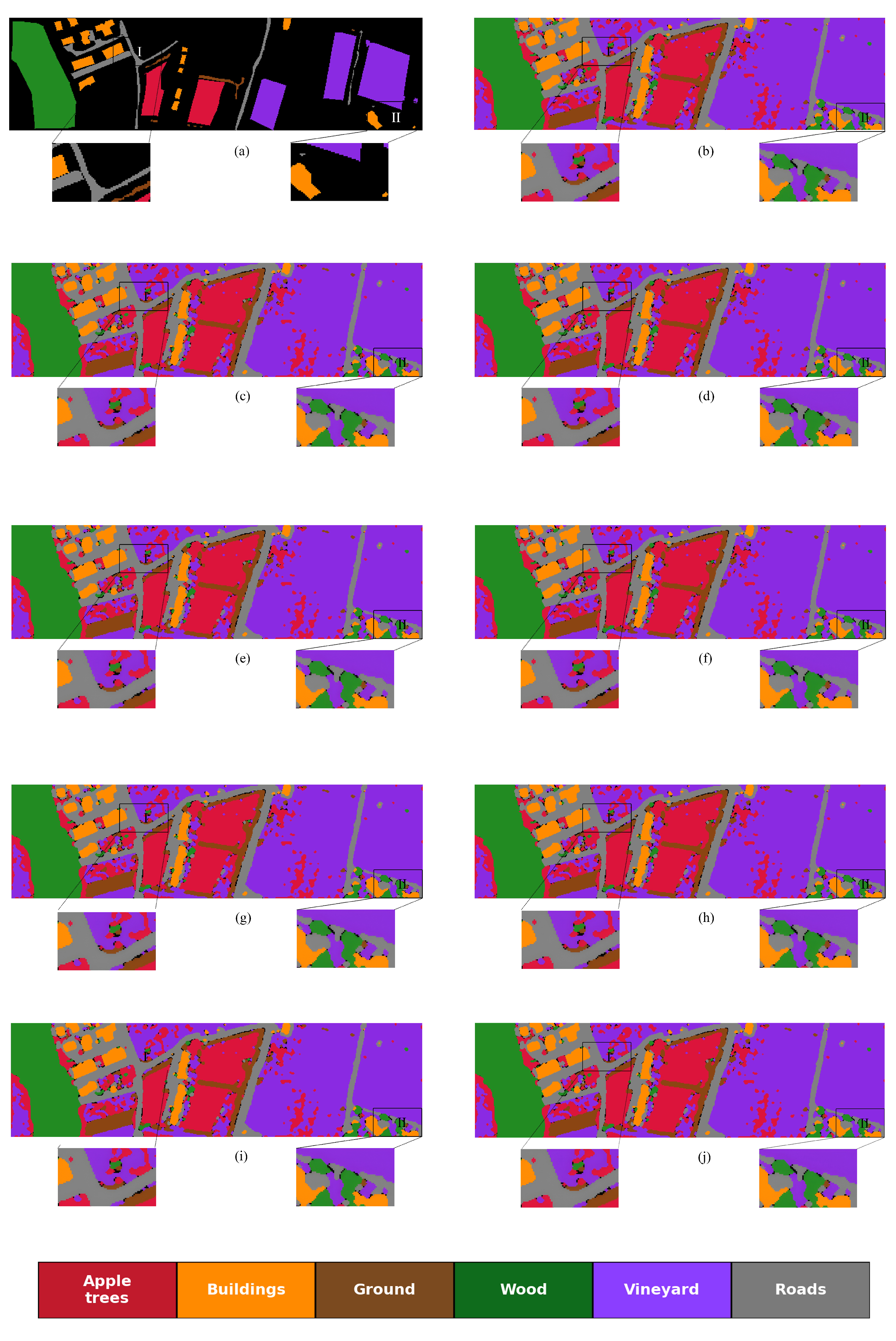
On each dataset, GL-Mamba outperformed all approaches in overall accuracy, average accuracy, and Kappa. This demonstrates that the network’s spectral–spatial feature extraction and hierarchical fusion capabilities effectively model complex interactions in hyperspectral-LiDAR data. The results on Houston2013 show particularly notable improvements over competing methods, highlighting GL-Mamba’s robustness in classifying diverse urban and vegetation classes. Visual inspection of classification maps (Figure 7, Figure 8 and Figure 9) shows that GL-Mamba produces less noise and smoother boundaries than competing networks. Table 3 presents class-level accuracy along with OA, AA, and Kappa for each dataset.

3.4.1. Classification Efficacy on the Trento Dataset

The Trento dataset contains agricultural fields and urban structures, with classes showing high spectral similarity such as vineyards and roads. According to Table 3, GL-Mamba achieves the best results: OA = 99.71%, AA = 99.52%, Kappa = 99.61. S3F2Net (OA = 99.70%) and DSHF (99.13%) are competitive but do not reach the same level. GL-Mamba achieves perfect or near-perfect classification for almost every class: 100% on Ground, Woods, and Roads, and 99.96% for Vineyard. S3F2Net achieves slightly higher accuracy on Building (99.21% vs. 98.13%), but does not match GL-Mamba’s overall performance across other classes.
The superiority of GL-Mamba is clearly reflected in the Trento classification maps in Figure 7. In Region I, where buildings, roads, and surrounding orchards are tightly interwoven, most competing methods produce broken road segments and mixed labels along boundaries. In contrast, GL-Mamba yields continuous roads, well-separated building blocks, and cleaner orchard parcels with minimal spurious pixels at class transitions. In Region II, which focuses on the interface between vineyards, ground, and roads, our method preserves both narrow road structures and regular vineyard shapes, whereas other approaches tend to oversmooth boundaries or introduce salt-and-pepper noise.

3.4.2. Classification Efficacy on the Augsburg Dataset

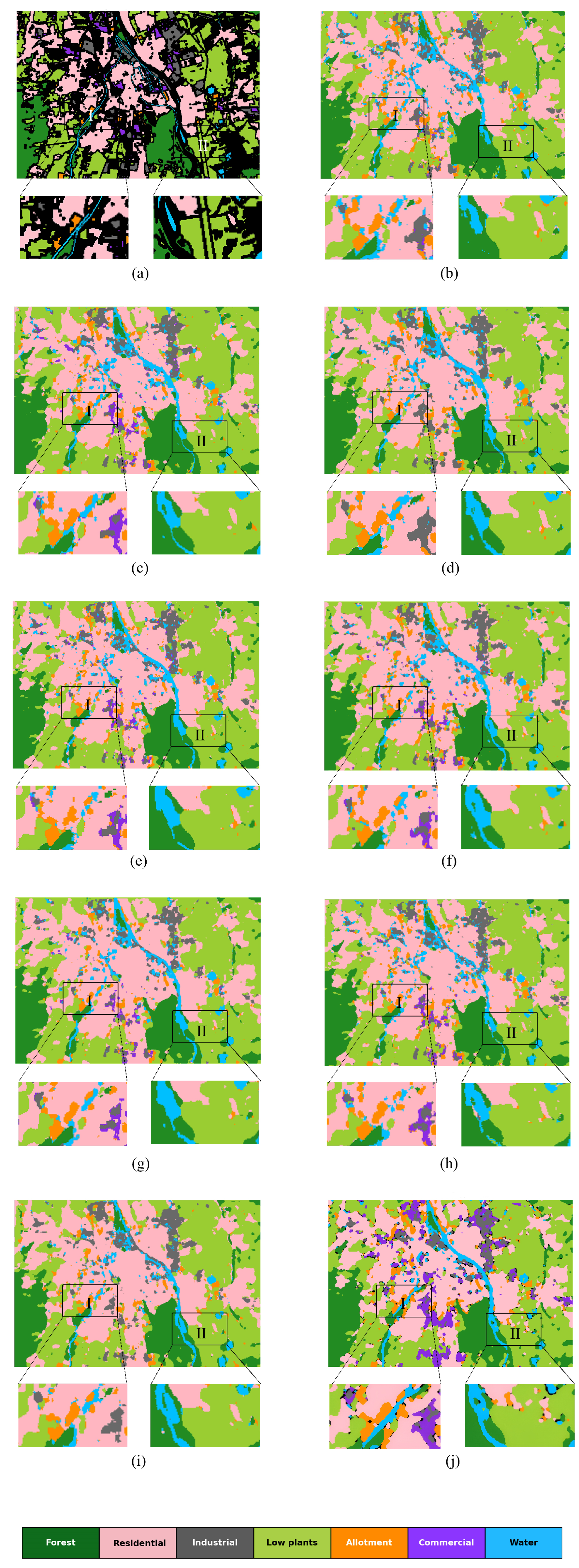
The Augsburg dataset contains multiple land-cover classes with vegetation, built structures, and small commercial parcels. GL-Mamba exhibits the highest overall metrics: OA = 94.58%, AA = 77.85%, and Kappa = 92.50%. Specifically, it achieves the highest accuracy in Forest (99.28%) and Water (62.57%) classes, with strong performance for Low-Plants (97.58%). Some baselines outperform GL-Mamba in specific classes: S3F2Net achieves higher Residential-Area accuracy (98.24% vs. 97.22%) and Allotment accuracy (96.94% vs. 92.54%), while DSHF provides the highest Industrial-Area accuracy (87.13% vs. 79.03%). The Commercial-Area class shows low accuracies across all methods due to limited training data (only 7 training pixels). Despite these isolated cases, GL-Mamba achieves the highest OA and Kappa, considerably ahead of DSHF (OA = 91.67%), MS2CANet (OA = 91.65%), and SAL2RN (OA = 89.85%).
A similar trend is observed in Figure 8. Region I focuses on a complex urban block where residential, industrial, and commercial parcels are interspersed. GL-Mamba shows compact residential neighbourhoods, clearer industrial patches, and more continuous road networks. Region II highlights the river corridor, where GL-Mamba delineates water more sharply and maintains homogeneous adjacent vegetation types.

3.4.3. Classification Efficacy on the Houston2013 Dataset

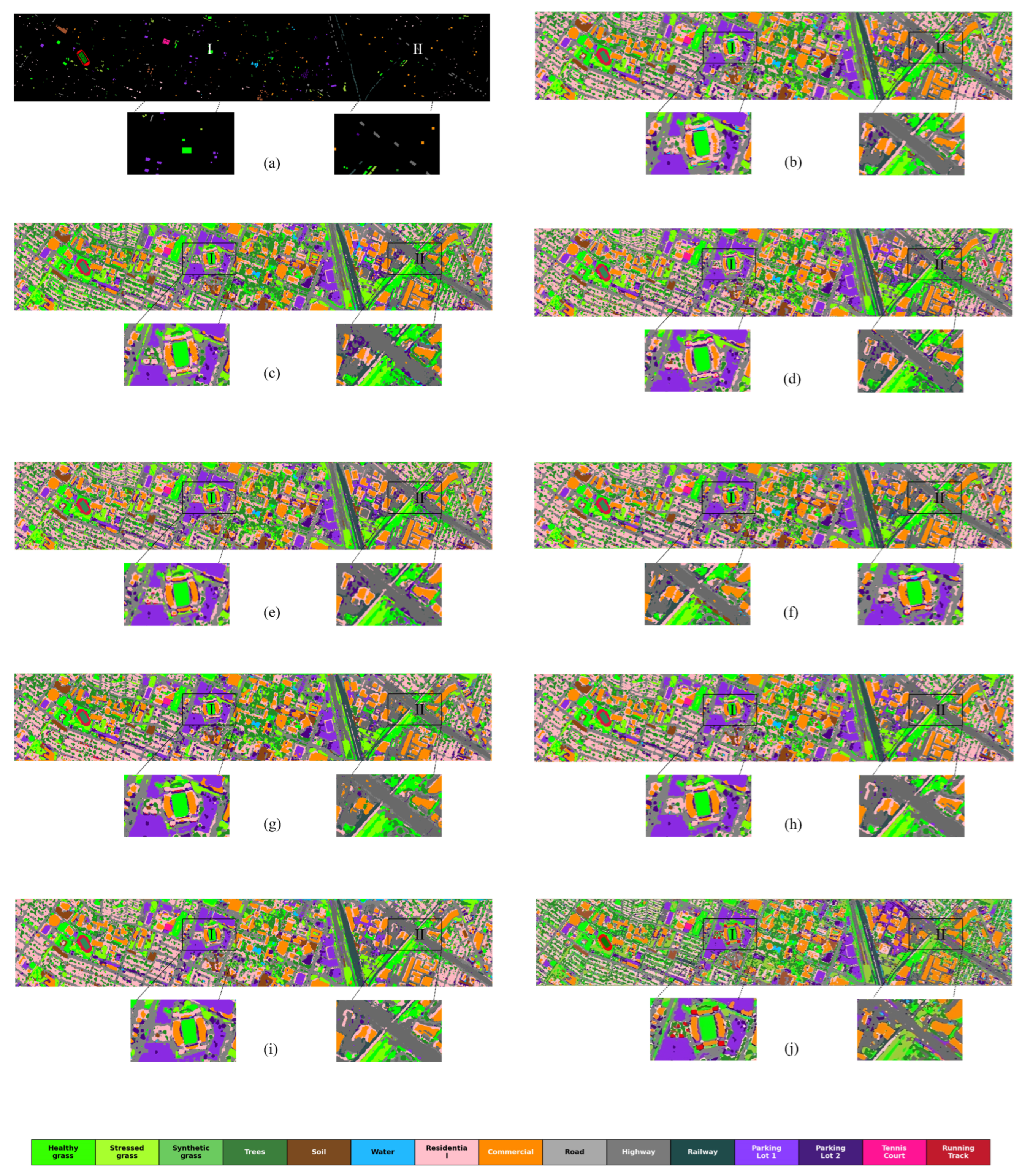
The Houston2013 dataset is notoriously challenging, with urban infrastructure intertwined with vegetation. As shown in Table 3, GL-Mamba achieves OA = 99.60%, AA = 99.68%, and Kappa = 99.56, far exceeding all baselines. It achieves near-perfect accuracies on almost all classes: Soil and Railway reach 100%, while Healthy grass, Synthetic grass, Trees, Residential, Highway, Tennis court, and Running track exceed 99.6%. All other baselines remain below 93% OA, with CCR-Net and DHViT achieving less than 91% OA due to limitations with long-range dependencies.
The visual comparison in Figure 9 confirms these advantages. Region I centers on the stadium area, where GL-Mamba sharply recovers fine structures of running tracks and tennis courts with uniform labels and well-aligned boundaries. Region II shows a densely built corridor where GL-Mamba produces a coherent highway network, clearly identifiable parking areas, and better separation from adjacent vegetation classes.
The classification maps demonstrate significant reduction in misclassification errors compared to other approaches. GL-Mamba shows clear advantages in preserving spatial coherence and reducing classification noise in both urban and rural settings. The global–local Mamba blocks, frequency-decomposed dual branches, and cross-attention fusion enable more effective extraction and integration of complementary spectral–spatial information than existing 3D CNNs, transformer hybrids, and graph-based networks.

3.4.4. Analysis of Class-Specific Limitations

While GL-Mamba achieves the highest overall accuracy across all datasets, we analyse classes where it shows relatively lower performance compared to specific baselines:
  • Commercial-Area in Augsburg (1.83%): This class has extremely limited training samples (only 7 pixels), making it nearly impossible for any deep learning method to learn meaningful representations. All baseline methods also perform poorly on this class, indicating a data scarcity issue rather than a model limitation.
  • Industrial-Area in Augsburg (79.03% vs. DSHF’s 87.13%): Industrial areas often contain mixed materials (metal roofs, concrete, vegetation) with high intra-class variability. DSHF’s hierarchical separation may handle such heterogeneity better, while GL-Mamba’s frequency decomposition may over-smooth some distinguishing texture patterns in these complex regions.
  • Building in Trento (98.13% vs. S3F2Net’s 99.21%): Buildings adjacent to roads share similar spectral characteristics, and the small accuracy gap (1.08%) reflects inherent ambiguity at class boundaries rather than a fundamental limitation.
Despite these isolated cases, GL-Mamba achieves the highest overall accuracy across all datasets, indicating that its strengths in the majority of classes more than compensate for these specific limitations.

3.5. Feature Visualization Analysis

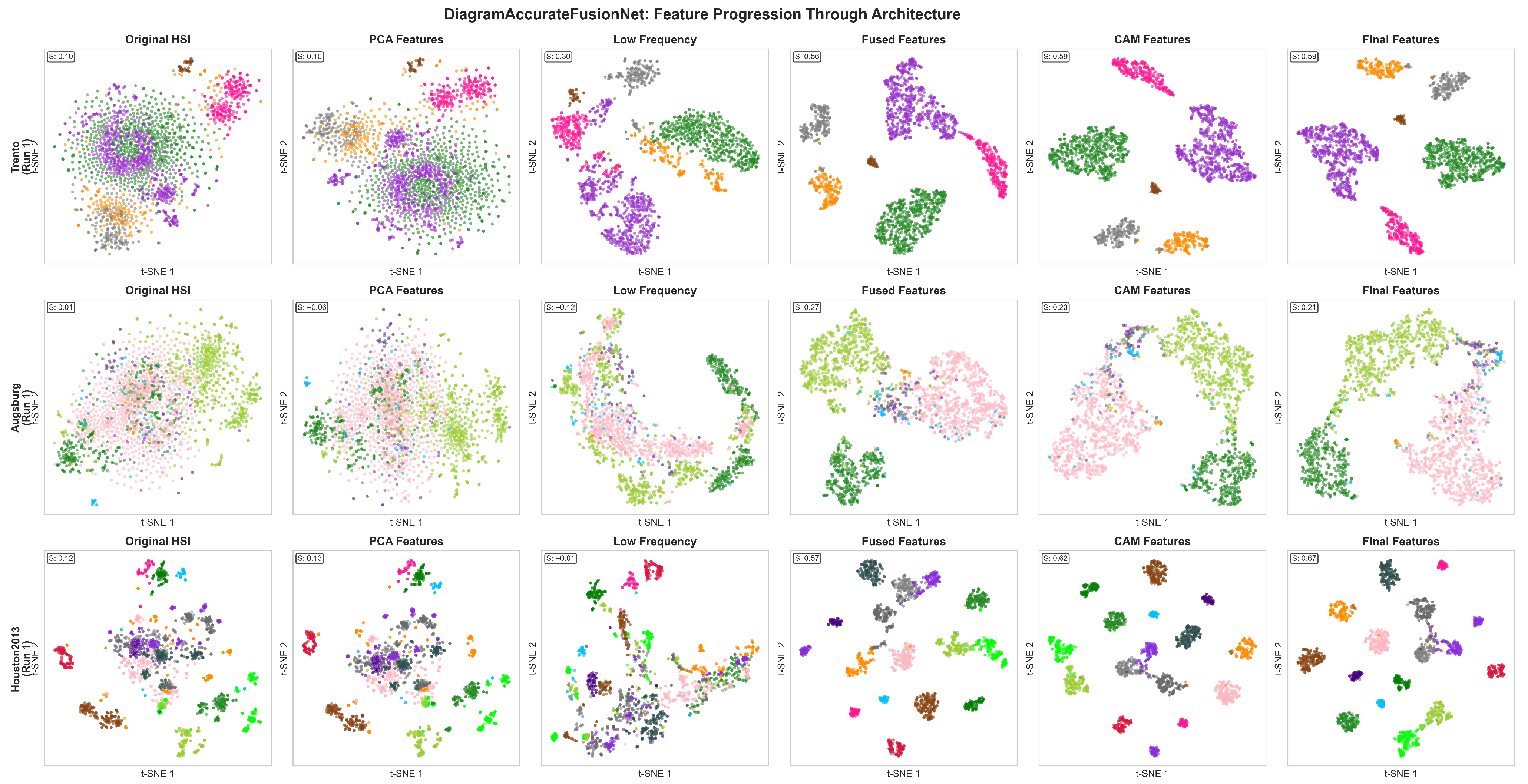
To intuitively examine how GL-Mamba transforms hyperspectral-LiDAR data, we used t-Distributed Stochastic Neighbour Embedding (t-SNE) to visualize features at each network stage. Figure 10 presents representative results for Trento, Augsburg, and Houston2013, showing the original HSI features, PCA-reduced representation, low-frequency branch outputs, fused features, cross-attention features, and final outputs.
In the original HSI plots, considerable class overlap exists. For example, in Trento, apple-tree, vineyard, building, and road classes overlap considerably; in Augsburg, farmland and orchard classes intermix; in Houston2013, commercial, residential, parking, and vegetation clusters overlap. PCA and the low-frequency branch alone provide limited class separation.
After dual-frequency processing and Mamba-based fusion, the results differ dramatically. The fused features become compact and distinct—in Trento, apple trees are clearly separated from vineyards, roads, and buildings; in Augsburg, agriculture is distinct from residential areas; in Houston2013, commercial areas separate from residential, roads, and vegetation. These results demonstrate the ability of Mamba-style state-space models to capture long-range dependencies while preserving local detail.
The cross-attention module further refines the embeddings. When LiDAR features query hyperspectral features, cross-attention decorrelates spectral redundancy and enhances class boundaries. In the CAM plots, classes form compact, well-separated clusters, indicating the network has learned to associate spectral signatures with elevation cues. The final features preserve or improve class separation, demonstrating that the complete GL-Mamba pipeline transforms the data into a feature space where classes are clearly distinguishable.

3.6. Computational Efficiency Analysis

To provide a fair and comprehensive comparison, we analyse the computational cost of GL-Mamba against all baseline methods. Table 4 reports the number of trainable parameters, floating-point operations (FLOPs), training time, and testing time on the Houston2013 dataset.
The results show that the proposed GL-Mamba achieves state-of-the-art accuracy (99.60% OA) with moderate computational cost. While the training time is higher due to the three-stage Mamba fusion process, the test time (2.07 s) remains competitive with other methods. The parameter count (275.20 K) is significantly lower than transformer-heavy methods like DHViT (3737.71 K) and SAL2RN (940.79 K), demonstrating the efficiency of our linear-complexity Mamba blocks. This favorable accuracy–efficiency trade-off makes GL-Mamba practical for real-world remote sensing applications.

4. Discussion

This section provides comprehensive analysis and interpretation of the experimental results.

4.1. Ablation Study

To evaluate the contribution of each component in the proposed GL-Mamba framework, we conduct comprehensive ablation experiments on three benchmark datasets: Houston2013, Augsburg, and Trento. The ablation study examines the influence of input modalities (HSI, LiDAR), architectural components (frequency decomposition, GL-Mamba fusion, cross-attention module), and their combinations on classification performance. Table 5 presents the results in terms of Overall Accuracy (OA), Average Accuracy (AA), and Kappa coefficient.

4.2. Impact of Input Modalities

We first analyze the contribution of each input modality. Using HSI alone achieves OA of 98.98%, 93.79%, and 98.88% on Trento, Augsburg, and Houston2013, respectively. The rich spectral information in HSI provides strong discriminative capability for land-cover classification. LiDAR-only classification yields lower performance (OA of 87.23%, 78.45%, and 83.67%), as elevation information alone lacks spectral signatures necessary for distinguishing spectrally similar classes. However, combining HSI and LiDAR improves performance across all datasets, demonstrating the complementary nature of spectral and elevation information.

4.3. Impact of Frequency Decomposition

The frequency-aware decomposition separates features into low-frequency (smooth variations) and high-frequency (fine details) components. Using only the low-frequency branch (CNN-based) achieves OA of 97.83%, 91.24%, and 97.12% on Trento, Augsburg, and Houston2013, respectively. The high-frequency branch (Transformer-based) alone yields OA of 96.45%, 89.67%, and 95.89%. Combining both branches through our dual-frequency design improves performance significantly, confirming that separating and independently processing frequency components captures complementary spectral–spatial patterns.

4.4. Impact of GL-Mamba Module

The GL-Mamba fusion module plays a critical role in capturing long-range dependencies while preserving local details. Without GL-Mamba (HSI+LiDAR direct fusion), OA drops to 99.27%, 93.10%, and 98.58% on Trento, Augsburg, and Houston2013. Adding GL-Mamba to HSI-only input improves OA to 99.16%, 93.23%, and 99.18%, demonstrating that the state-space model effectively refines single-modality features. The full model with HSI, LiDAR, and GL-Mamba achieves the best results (OA of 99.71%, 94.58%, and 99.60%), confirming that GL-Mamba effectively aligns and integrates complementary information from both modalities.

4.5. Impact of Cross-Attention Module

The cross-attention module (CAM) enables information exchange between HSI and LiDAR features. Removing CAM while retaining other components reduces OA to 99.48%, 93.92%, and 99.31% on Trento, Augsburg, and Houston2013. This demonstrates that cross-modal attention helps decorrelate spectral redundancy and enhances class boundaries by associating spectral signatures with elevation cues, as visualized in the t-SNE analysis (Figure 10).

4.6. Summary of Ablation Results

The complete GL-Mamba framework integrating all components achieves the best performance across all datasets and metrics. Each component contributes measurably to the final results: frequency decomposition enables specialized processing of different spectral–spatial patterns, GL-Mamba captures long-range dependencies with linear complexity, and cross-attention bridges the semantic gap between modalities. The progressive improvement from Original HSI → PCA → Low-Frequency → Fused → CAM → Final features, as shown in the t-SNE visualization, align with these quantitative ablation results.

4.7. Isolated Contribution Analysis

To directly address the distinct contributions of GL-Mamba and cross-attention, we highlight the following comparisons from Table 5:
Contribution of GL-Mamba (comparing Row 5 vs. Row 7):
  • Without GL-Mamba: OA = 99.27% (Trento), 93.10% (Augsburg), 98.58% (Houston)
  • With GL-Mamba (no CAM): OA = 99.48%, 93.92%, 99.31%
  • Improvement:+0.21%, +0.82%, +0.73%
Contribution of Cross-Attention Module (comparing Row 7 vs. Row 8):
  • Without CAM: OA = 99.48% (Trento), 93.92% (Augsburg), 99.31% (Houston)
  • With CAM (full model): OA = 99.71%, 94.58%, 99.60%
  • Improvement: +0.23%, +0.66%, +0.29%
These results demonstrate that both components provide complementary benefits: GL-Mamba contributes larger gains on Augsburg and Houston2013 (complex scenes with long-range dependencies), while CAM provides consistent refinement across all datasets by enabling cross-modal information exchange.

5. Conclusions

This paper presented GL-Mamba, a global–local Mamba-based dual-modality fusion network for hyperspectral and LiDAR data classification. The framework integrates frequency-aware decomposition, lightweight CNN/Transformer branches, a Global–Local Mamba state-space block, and a cross-attention bridge to exploit complementary spectral, spatial, and elevation information in a unified manner. Experiments on the Trento, Augsburg, and Houston2013 datasets demonstrated consistent state-of-the-art performance over eight recent baselines, with overall accuracies of 99.71%, 94.58%, and 99.60%, respectively. Ablation studies confirmed the contribution of each component to the final accuracy and boundary quality.
Several limitations should be acknowledged. GL-Mamba assumes accurate HSI–LiDAR co-registration, relies on supervised training with sufficient labelled data, and requires careful selection of patch size and stride; moreover, very large or ultra-high-resolution scenes remain computationally demanding. Nevertheless, the linear-complexity sequence modelling and dual-frequency design provide a favourable trade-off between accuracy and efficiency, making GL-Mamba a promising candidate for practical land-cover mapping and edge deployment. Future work will investigate multi-scale and dynamic Mamba designs, semi- or weakly supervised learning, and the integration of additional modalities (e.g., SAR or multispectral imagery) to further improve robustness and scalability.

Author Contributions

Conceptualization, K.M.H. and Y.L.; methodology, K.M.H.; software, K.M.H. and K.Z.; validation, K.M.H., K.Z. and S.P.; formal analysis, K.M.H.; investigation, K.M.H.; resources, Y.L.; data curation, K.M.H. and S.P.; writing—original draft preparation, K.M.H.; writing—review and editing, K.Z., S.P. and Y.L.; visualization, K.M.H.; supervision, Y.L.; project administration, Y.L. All authors have read and agreed to the published version of the manuscript.

Funding

This research received no external funding.

Data Availability Statement

The Houston2013 dataset is publicly available from the IEEE GRSS Data Fusion Contest (Available online: https://www.grss-ieee.org/community/technical-committees/2013-ieee-grss-data-fusion-contest/, accessed on 15 January 2023). The Trento and Augsburg datasets are available from the corresponding references cited in the manuscript. The proposed model was implemented using Python 3.10 and the PyTorch 2.0.1 deep-learning framework with CUDA 11.8 support. The code and trained models will be made available upon reasonable request to the corresponding author.

Conflicts of Interest

The authors declare no conflicts of interest.

References

  1. Qu, K.; Wang, H.; Ding, M.; Luo, X.; Bao, W. DGMNet: Hyperspectral Unmixing Dual-Branch Network Integrating Adaptive Hop-Aware GCN and Neighborhood Offset Mamba. Remote Sens. 2025, 17, 2517. [Google Scholar] [CrossRef]
  2. Huo, Y.; Cheng, X.; Lin, S.; Zhang, M.; Wang, H. Memory-Augmented Autoencoder with Adaptive Reconstruction and Sample Attribution Mining for Hyperspectral Anomaly Detection. IEEE Trans. Geosci. Remote Sens. 2024, 62, 5518118. [Google Scholar] [CrossRef]
  3. Cai, Q.; Qu, J.; Dong, W.; Yang, Y. Interpretable Low-Rank Sparse Unmixing and Spatial Attention-Enhanced Difference Mapping Network for Hyperspectral Change Detection. IEEE Trans. Geosci. Remote Sens. 2025, 63, 5526414. [Google Scholar] [CrossRef]
  4. Hussain, K.M.; Zhao, K.; Zhou, Y.; Ali, A.; Li, Y. Cross Attention Based Dual-Modality Collaboration for Hyperspectral Image and LiDAR Data Classification. Remote Sens. 2025, 17, 2836. [Google Scholar] [CrossRef]
  5. Li, S.; Huang, S. AFA–Mamba: Adaptive Feature Alignment with Global–Local Mamba for Hyperspectral and LiDAR Data Classification. Remote Sens. 2024, 16, 4050. [Google Scholar] [CrossRef]
  6. Yang, J.X.; Zhou, J.; Wang, J.; Tian, H.; Liew, A.W. LiDAR-Guided Cross-Attention Fusion for Hyperspectral Band Selection and Image Classification. arXiv 2024, arXiv:2404.03883. [Google Scholar]
  7. Yang, J.X.; Wang, J.; Sui, C.H.; Long, Z.; Zhou, J. HSLiNets: Hyperspectral Image and LiDAR Data Fusion Using Efficient Dual Non-Linear Feature Learning Networks. arXiv 2024, arXiv:2412.00302. [Google Scholar]
  8. Gao, F.; Jin, X.; Zhou, X.; Dong, J.; Du, Q. MSFMamba: Multi-Scale Feature Fusion State Space Model for Multi-Source Remote Sensing Image Classification. arXiv 2024, arXiv:2408.14255. [Google Scholar]
  9. Wang, M.; Wu, Q.; Zhou, S.; Yu, F.; Zhu, J.; Lu, H. Joint Classification of Hyperspectral and LiDAR Data Based on Adaptive Gating Mechanism and Learnable Transformer. Remote Sens. 2024, 16, 1080. [Google Scholar] [CrossRef]
  10. Wang, Q.; Zhou, B.; Zhang, J.; Xie, J.; Wang, Y. Joint Classification of Hyperspectral Images and LiDAR Data Based on Dual-Branch Transformer. Sensors 2024, 24, 867. [Google Scholar] [CrossRef] [PubMed]
  11. Zhang, S.; Wang, Y.; Li, W.; Gao, L.; Li, P.; Tao, T. Feature-Decision Level Collaborative Fusion Network for Hyperspectral and LiDAR Classification. Remote Sens. 2023, 15, 4148. [Google Scholar] [CrossRef]
  12. Han, W.; Li, Y.; Zhang, Q.; Yuan, Q.; Du, Q. Cross-Modal Semantic Enhancement Network for Classification of Hyperspectral and LiDAR Data. IEEE Trans. Geosci. Remote Sens. 2024, 62, 5509814. [Google Scholar] [CrossRef]
  13. Lu, T.; Dai, G.; Li, S.; Liang, X.; Zheng, X. Coupled Adversarial Learning for Fusion Classification of Hyperspectral and LiDAR Data. Inf. Fusion 2023, 93, 118–131. [Google Scholar] [CrossRef]
  14. Cai, J.; Xu, Y.; Wei, W.; Jia, X.; Xu, Y. A Novel Graph-Attention Based Multimodal Fusion Network for Joint Classification of Hyperspectral Image and LiDAR Data. Expert Syst. Appl. 2024, 249, 123587. [Google Scholar] [CrossRef]
  15. Ge, H.; Wang, J.; Zhao, Q.; Zhang, B. Cross Attention-Based Multi-Scale Convolutional Fusion Network for Hyperspectral and LiDAR Joint Classification. Remote Sens. 2024, 16, 4073. [Google Scholar] [CrossRef]
  16. Wang, F.; Li, C.; Zhang, J.; Zhang, Z.; Liang, Q. Remote Sensing LiDAR and Hyperspectral Classification with Multi-Scale Graph Encoder–Decoder Network. Remote Sens. 2024, 16, 3912. [Google Scholar] [CrossRef]
  17. Pan, H.; Wei, N.; Chen, P.; Su, L.; Dong, Q. Multiscale Adaptive Fusion Network for Joint Classification of Hyperspectral and LiDAR Data. Int. J. Remote Sens. 2025, 46, 6594–6634. [Google Scholar] [CrossRef]
  18. Pan, J.; Chen, T.; Tang, Y.; Li, H.; Guan, P. Classification of Hyperspectral and LiDAR Data by Transformer-Based Enhancement. Remote Sens. Lett. 2024, 15, 1074–1084. [Google Scholar] [CrossRef]
  19. Wang, L.; Deng, S. Hypergraph Convolution Network Classification for Hyperspectral and LiDAR Data. Sensors 2025, 25, 3092. [Google Scholar] [CrossRef]
  20. Taukiri, A.; Pouliot, D.; Rospars, M.; Crawford, G.; McDonough, K.; Glover, S.; Westwood, E. FusionFormer-X: Hierarchical Self-Attentive Multimodal Transformer for HSI–LiDAR Remote Sensing Scene Understanding. Preprints 2025. [Google Scholar] [CrossRef]
  21. Li, Z.; Liu, R.; Zhou, S.; Zheng, Y.; Wang, Y. Multi-Feature Cross Attention-Induced Transformer Network for Hyperspectral and LiDAR Data Classification. Remote Sens. 2024, 16, 2775. [Google Scholar] [CrossRef]
  22. Liu, J.; Li, Y.; Zhang, T.; Liu, M.; Zhang, Y. Classification of Hyperspectral–LiDAR Dual-View Data Using Hybrid Feature and Trusted Decision Fusion. Remote Sens. 2024, 16, 4381. [Google Scholar] [CrossRef]
  23. Long, F.; Chen, F.; Yao, J.; Du, Q.; Pu, Y. Multimodal Prompt Tuning for Hyperspectral and LiDAR Classification. Remote Sens. 2025, 17, 2826. [Google Scholar] [CrossRef]
  24. Li, Y.; Li, W.; Gong, L.; Zhao, X.; Wang, B. Multiscale Attention Feature Fusion Based on Improved Transformer for Hyperspectral Image and LiDAR Data Classification. IEEE J. Sel. Top. Appl. Earth Obs. Remote Sens. 2025, 18, 4124–4140. [Google Scholar] [CrossRef]
  25. Wang, H.; Cheng, Y.; Liu, X.; Wang, X. Reinforcement Learning Based Markov Edge Decoupled Fusion Network for Fusion Classification of Hyperspectral and LiDAR. IEEE Trans. Multimed. 2024, 26, 7174–7187. [Google Scholar] [CrossRef]
  26. Cai, Y.; Zheng, H.; Luo, J.; Fan, L.; Li, H. Learning Unified Anchor Graph for Joint Clustering of Hyperspectral and LiDAR Data. IEEE Trans. Neural Netw. Learn. Syst. 2025, 36, 6341–6354. [Google Scholar] [CrossRef] [PubMed]
  27. Roy, S.K.; Krishna, G.; Dubey, S.R.; Chaudhuri, B.B. Cross Hyperspectral and LiDAR Attention Transformer for Multimodal Remote Sensing Classification. IEEE Trans. Geosci. Remote Sens. 2024, 62, 5512815. [Google Scholar] [CrossRef]
  28. Wang, L.; Meng, C.; Zhou, Y.; Zhang, Y. Interactive Transformer and CNN Network for Fusion Classification of Hyperspectral and LiDAR Data. Int. J. Remote Sens. 2024, 45, 9235–9266. [Google Scholar] [CrossRef]
  29. Zhao, Y.; Sun, H.; Kang, G.; Li, J.; Gao, X. Local-to-Global Cross-Modal Attention-Aware Fusion for HSI-X Data. arXiv 2024, arXiv:2406.17679. [Google Scholar]
  30. Butt, M.H.F.; Li, J.; Han, Y.; Shi, C.; Zhu, F.; Huang, L. Graph-Infused Hybrid Vision Transformer: Advancing GeoAI for Enhanced Land Cover Classification. Int. J. Appl. Earth Obs. Geoinf. 2024, 124, 103773. [Google Scholar] [CrossRef]
  31. Zang, S.; Li, Q.; Deng, W.; Li, B. A Comprehensive Survey for Hyperspectral Image Classification in the Era of Deep Learning and Transformers. arXiv 2024, arXiv:2404.14955. [Google Scholar]
  32. Wang, S.; Hou, C.; Chen, Y.; Liu, Z.; Zhang, Z.; Zhang, G. Classification of Hyperspectral and LiDAR Data Using Multi-Modal Transformer Cascaded Fusion Net. Remote Sens. 2023, 15, 4142. [Google Scholar] [CrossRef]
  33. Liu, G.; Song, J.; Chu, Y.; Zhang, L.; Li, P.; Xia, J. Deep Fuzzy Fusion Network for Joint Hyperspectral and LiDAR Data Classification. Remote Sens. 2025, 17, 2923. [Google Scholar] [CrossRef]
  34. Wang, Z.; Wang, Q.; Zhang, J.; Liang, X. Joint Classification of Hyperspectral and LiDAR Data Based on Heterogeneous Attention Feature Fusion Network. In Proceedings of the IGARSS 2024—2024 IEEE International Geoscience and Remote Sensing Symposium, Athens, Greece, 7–12 July 2024; pp. 1–4. [Google Scholar] [CrossRef]
  35. Rizaldy, A.; Gloaguen, R.; Fassnacht, F.E.; Ghamisi, P. HyperPointFormer: Multimodal Fusion in 3D Space with Dual-Branch Cross-Attention Transformers. arXiv 2025, arXiv:2505.23206. [Google Scholar]
  36. Liao, D.; Wang, Q.; Lai, T.; Huang, H. Joint Classification of Hyperspectral and LiDAR Data Based on Mamba. IEEE Trans. Geosci. Remote Sens. 2024, 62, 5530915. [Google Scholar] [CrossRef]
  37. Song, T.; Zeng, Z.; Gao, C.; Chen, H.; Ma, X. Joint Classification of Hyperspectral and LiDAR Data Using Height Information Guided Hierarchical Fusion-and-Separation Network. IEEE Trans. Geosci. Remote Sens. 2024, 62, 5505315. [Google Scholar] [CrossRef]
  38. Zeng, Z.; Song, T.; Ma, X.; Jiu, Y.; Sun, H. Joint Classification of Hyperspectral and Lidar Data Using Cross-Modal Hierarchical Frequency Fusion Network. In Proceedings of the ICASSP 2024—2024 IEEE International Conference on Acoustics, Speech and Signal Processing (ICASSP), Seoul, Republic of Korea, 14–19 April 2024; pp. 1–5. [Google Scholar] [CrossRef]
  39. Zhang, M.; Li, W.; Zhang, Y.; Tao, R.; Du, Q. Hyperspectral and LiDAR Data Classification Based on Structural Optimization Transmission. IEEE Trans. Cybern. 2023, 53, 3153–3164. [Google Scholar] [CrossRef] [PubMed]
  40. Gao, Y.; Li, W.; Wang, J.; Zhang, M.; Tao, R. Distribution-Independent Domain Generalization for Multisource Remote Sensing Classification. IEEE Trans. Neural Netw. Learn. Syst. 2024, 36, 13333–13344. [Google Scholar] [CrossRef] [PubMed]
  41. Debes, C.; Merentitis, A.; Heremans, R.; Hahn, J.; Frangiadakis, N.; Van Kasteren, T.; Liao, W.; Bellens, R.; Pižurica, A.; Gautama, S.; et al. Hyperspectral and LiDAR data fusion: Outcome of the 2013 GRSS data fusion contest. IEEE J. Sel. Top. Appl. Earth Obs. Remote Sens. 2014, 7, 2405–2418. [Google Scholar] [CrossRef]
  42. Hong, D.; Gao, L.; Hang, R.; Zhang, B.; Chanussot, J. Deep encoder–decoder networks for classification of hyperspectral and LiDAR data. IEEE Geosci. Remote Sens. Lett. 2020, 19, 5500205. [Google Scholar] [CrossRef]
  43. Hong, D.; Hu, J.; Yao, J.; Chanussot, J.; Zhu, X.X. Multimodal remote sensing benchmark datasets for land cover classification with a shared and specific feature learning model. ISPRS J. Photogramm. Remote Sens. 2021, 178, 68–80. [Google Scholar] [CrossRef]
  44. Wu, X.; Hong, D.; Chanussot, J. Convolutional neural networks for multimodal remote sensing data classification. IEEE Trans. Geosci. Remote Sens. 2021, 60, 5517010. [Google Scholar] [CrossRef]
  45. Yao, J.; Zhang, B.; Li, C.; Hong, D.; Chanussot, J. Extended vision transformer (ExViT) for land use and land cover classification: A multimodal deep learning framework. IEEE Trans. Geosci. Remote Sens. 2023, 61, 5514415. [Google Scholar] [CrossRef]
  46. Xue, Z.; Tan, X.; Yu, X.; Liu, B.; Yu, A.; Zhang, P. Deep hierarchical vision transformer for hyperspectral and LiDAR data classification. IEEE Trans. Image Process. 2022, 31, 3095–3110. [Google Scholar] [CrossRef]
  47. Li, X.; Li, Y.; Zhang, L. SAL2RN: Spectral–And–LiDAR Two-Branch Residual Network for HSI–LiDAR Classification. Remote Sens. 2022, 14, 4090. [Google Scholar] [CrossRef]
  48. Wang, X.; Zhu, J.; Feng, Y.; Wang, L. MS2CANet: Multiscale Spatial–Spectral Cross-Modal Attention Network for Hyperspectral and LiDAR Data Classification. IEEE Geosci. Remote Sens. Lett. 2024, 21, 5500505. [Google Scholar] [CrossRef]
  49. Feng, Y.; Song, L.; Wang, L.; Wang, X. DSHFNet: Dynamic Scale Hierarchical Fusion Network Based on Multiattention for Hyperspectral Image and LiDAR Data Classification. IEEE Trans. Geosci. Remote Sens. 2023, 61, 5522514. [Google Scholar] [CrossRef]
  50. Wang, X.; Song, L.; Feng, Y.; Zhu, J. S3F2Net: Spatial-Spectral-Structural Feature Fusion Network for Hyperspectral Image and LiDAR Data Classification. IEEE Trans. Circuits Syst. Video Technol. 2025, 35, 4801–4815. [Google Scholar] [CrossRef]
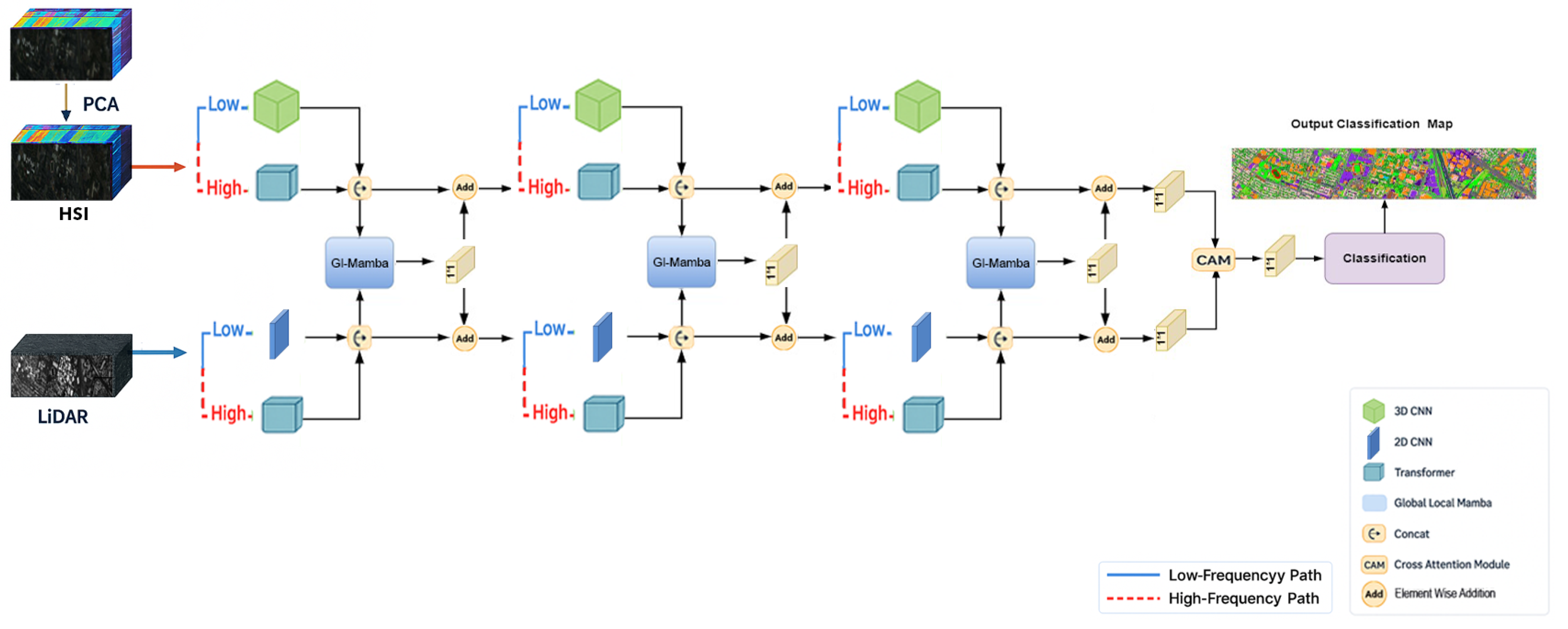
Figure 1. Overall architecture of the proposed GL-Mamba framework for HSI–LiDAR classification. The model employs frequency-aware decomposition, dual-branch feature extraction, three-stage GL-Mamba fusion, and cross-attention bridging.
Remotesensing 18 00138 g001
Figure 2. Architecture of the GL-Mamba fusion module showing the global branch, local branch, and their integration through concatenation and gating mechanisms.
Remotesensing 18 00138 g002
Figure 3. Detailed architecture of the Simplified Mamba Block. The block employs a State Space Model (SSM) with learnable matrices ( A , B , C , D ) and selective scanning to capture long-range dependencies with linear O ( L ) complexity. The state recurrence follows h t = A ¯ h t 1 + B ¯ u t , with gated fusion combining the SSM output and 1D convolution features through element-wise multiplication.
Remotesensing 18 00138 g003
Figure 4. Cross-attention module (CAM) for HSI–LiDAR feature fusion. HSI features serve as queries while LiDAR features provide keys and values, enabling spectral-elevation information exchange.
Remotesensing 18 00138 g004
Figure 5. Comparison of patch size with OA on benchmark datasets.Augsburg, Houston2013, and Trento.
Remotesensing 18 00138 g005
Figure 6. Comparison of different learning rates on benchmark datasets. (a) Trento. (b) Augsburg. (c) Houston2013.
Remotesensing 18 00138 g006
Figure 7. Classification maps for the Trento dataset: (a) Ground Truth; (b) CCR-Net; (c) CALC; (d) ExViT; (e) DHViT; (f) SAL2RN; (g) MS2CANet; (h) DSHF; (i) S3F2Net; (j) Proposed GL-Mamba (99.71%). Regions I and II show zoomed areas for detailed comparison.
Remotesensing 18 00138 g007
Figure 8. Classification maps for the Augsburg dataset: (a) Ground Truth; (b) CCR-Net; (c) CALC; (d) ExViT; (e) DHViT; (f) SAL2RN; (g) MS2CANet; (h) DSHF; (i) S3F2Net; (j) Proposed GL-Mamba (94.58%). Regions I and II show zoomed areas for detailed comparison.
Remotesensing 18 00138 g008
Figure 9. Classification maps for the Houston2013 dataset: (a) Ground Truth; (b) CCR-Net; (c) CALC; (d) ExViT; (e) DHViT; (f) SAL2RN; (g) MS2CANet; (h) DSHF; (i) S3F2Net; (j) Proposed GL-Mamba (99.60%). Regions I and II show zoomed areas for detailed comparison.
Remotesensing 18 00138 g009
Figure 10. t-SNE visualization of feature distributions at different network stages for Trento, Augsburg, and Houston2013 datasets.
Remotesensing 18 00138 g010
Table 1. Summary of notations used in this paper.
SymbolsDefinitions
X H , X L Original hyperspectral image (HSI) cube and LiDAR raster of the scene
H , W Height and width of the HSI/LiDAR images
BNumber of HSI spectral bands after PCA
SSpatial patch size ( S     S )
CNumber of land-cover classes
x i H , x i L HSI and LiDAR patches centred at the i-th pixel
x i Dual-modality input of the i-th sample, x i = ( x i H , x i L )
y i true , y ^ i Ground-truth label and predicted class-probability vector of the i-th sample
F H low , F H high Low-/high-frequency HSI features (3D CNN/transformer)
F L low , F L high Low-/high-frequency LiDAR features (2D CNN/transformer)
F H , F L Concatenated HSI and LiDAR embeddings after dual-frequency branches
U s Input feature sequence to the GL-Mamba fusion block at stage s
Z ( 1 ) , Z ( 2 ) , Z ( 3 ) Fused feature maps after the three GL-Mamba stages
F global Globally aggregated feature map from all fusion stages
Q , K , V Query, key and value matrices in the cross-attention bridge
F fused Output feature map of the cross-attention module
Δ Predicted spatial offset field for cross-modal alignment
warp ( · , Δ ) Warping operator that aligns features using the offsets Δ
L Cross-entropy loss used for training
OA , AA , κ Overall accuracy, average accuracy and Kappa coefficient
Table 2. Dataset Description.
DatasetHouston2013 [41]Trento [42]Augsburg [43]
LocationHouston, TX, USATrento, ItalyAugsburg, Germany
Sensor TypeHSILiDARHSILiDARHSILiDAR
Image Size349 ✕ 1905349 ✕ 1905600 ✕ 166600 ✕ 166332 ✕ 485332 ✕ 485
Spatial Resolution2.5 m2.5 m1 m1 m30 m30 m
Number of Bands14416311801
Wavelength Range0.38–1.05  μ m/0.42–0.99  μ m/0.4–2.5  μ m/
Sensor NameCASI-1500/AISA EagleOptech ALTM 3100EAHySpexDLR-3K
Table 3. Classification accuracy comparison on Trento, Augsburg, and Houston2013 datasets. Best results in bold, second-best underlined.
(a) Trento Dataset
No.Class (Train/Test)CALCCCR-NetExViTDHViTSAL2RNMS2CANetDSHFS3F2NetGL-Mamba
1Apple trees (129/3905)97.26100.0099.5698.3699.7499.8499.4999.9599.95
2Building (125/2778)100.0098.8898.1399.0696.7698.5298.7499.2198.13
3Ground (105/374)89.5779.6876.4767.6583.686.3699.7397.59100.00
4Woods (154/8969)100.00100.00100.00100.00100.0099.2199.98100.00100.00
5Vineyard (184/10317)99.7594.7999.9398.8999.97100.00100.00100.0099.96
6Roads (122/3052)87.4588.0793.8487.9888.9992.9293.4598.2099.08
OA%98.1696.5798.8098.0098.0698.9299.1399.7099.71
AA%95.6893.5794.6692.1694.7296.2798.5799.1699.52
Kappa ✕ 10097.4895.4398.3997.3197.4098.5698.8399.5999.61
(b) Augsburg Dataset
No.Class (Train/Test)CALCCCR-NetExViTDHViTSAL2RNMS2CANetDSHFS3F2NetGL-Mamba
1Forest (146/13361)94.1693.4791.8390.4596.5896.4097.6098.7499.28
2Residential (264/30065)95.3296.8695.3890.8797.6997.9092.9498.2497.22
3Industrial (21/3830)86.1882.5643.3261.2053.4448.7987.1378.0979.03
4Low-Plants (248/36609)95.5784.4591.1382.8292.8496.4796.3897.5997.58
5Allotment (52/523)0.0044.3641.1121.8038.6244.5564.0596.9492.54
6Commercial (7/1638)6.050.0026.0123.5015.1413.432.5011.901.83
7Water (23/1507)55.9640.4842.077.4312.4749.9048.7758.3362.57
OA%91.4687.8287.8283.0689.8591.6591.6794.5094.58
AA%61.8963.1761.4154.0158.1163.9269.9177.1277.85
Kappa ✕ 10088.0482.4882.4475.9185.2688.2288.1292.1092.50
(c) Houston2013 Dataset
No.Class (Train/Test)CALCCCR-NetExViTDHViTSAL2RNMS2CANetDSHFS3F2NetGL-Mamba
1Healthy grass (198/1053)94.6494.6482.2485.1591.5581.0182.6285.7599.72
2Stressed grass (190/1064)94.5194.6483.9384.8790.8589.5193.4796.7199.44
3Synthetic grass (192/506)89.3779.4782.9979.7692.8799.6799.9195.8499.68
4Trees (188/1056)96.2590.7188.9092.9196.4794.5099.9198.2099.91
5Soil (188/1056)96.2594.0190.8592.6196.4093.88100.0099.71100.00
6Water (162/143)96.2591.4792.2194.3694.7292.12100.0097.9099.92
7Residential (196/1072)97.0092.9891.5095.9394.2492.5897.9095.2499.70
8Commercial (191/1053)95.5393.5394.0394.7292.6191.91100.0095.3499.62
9Road (193/1063)91.5492.8792.3391.9094.8394.5699.3296.3199.59
10Highway (191/1054)92.7793.3595.4091.3889.5794.7799.3281.8599.65
11Railway (181/1062)93.6391.7591.0993.4794.5095.58100.0097.62100.00
12Parking lot 1 (190/1054)91.0989.6491.7193.2291.5092.7599.6098.4699.74
13Parking lot 2 (119/1047)94.4587.8691.5792.2190.5193.0499.5294.3899.65
14Tennis court (181/247)95.3697.0695.5591.5295.0696.52100.0095.14100.00
15Running track (187/473)97.0999.8697.6299.1297.6296.61100.00100.0099.95
OA%91.0788.8885.7290.6689.8392.8891.6794.5099.60
AA%91.2091.2487.0991.1590.5091.0292.5091.7699.68
Kappa ✕ 10089.8987.8789.5288.4690.4290.8792.9192.2799.56
Table 4. Number of parameters and FLOPs, training and testing times on the Houston2013 dataset.
CCR-NetCALCExViTDHViTSAL2RNMS2CANetDSHFS3F2NetProposed
Params (K)70.08284.14229.103737.71940.79180.02312.45425.38275.20
FLOPs (M)0.1428.7546.87322.526.322.2318.6432.1757.50
Training time (s)61.12563.14323.86472.35163.70115.77198.42245.63688.64
Test time (s)0.062.044.275.811.781.561.822.352.07
Table 5. Ablation Study of GL-Mamba Architecture. Ticks () indicate enabled modules; crosses () indicate disabled modules. Best results are shown in bold.
ComponentsMetricsDatasets
HSI LiDAR Low-Freq High-Freq GL-Mamba CAM Trento Augsburg Houston2013
OA (%)98.9893.7998.88
AA (%)99.2275.4498.19
Kappa (%)98.9091.0698.50
OA (%)87.2378.4583.67
AA (%)84.5662.3181.24
Kappa (%)85.1272.8981.45
OA (%)97.8391.2497.12
AA (%)96.4571.5696.34
Kappa (%)97.2188.4596.78
OA (%)96.4589.6795.89
AA (%)95.1268.9294.56
Kappa (%)95.7886.2395.12
OA (%)99.2793.1098.58
AA (%)99.6777.1299.02
Kappa (%)99.5492.1099.50
OA (%)99.1693.2399.18
AA (%)98.5176.3799.10
Kappa (%)99.1490.1299.11
OA (%)99.4893.9299.31
AA (%)99.3477.4599.42
Kappa (%)99.4591.7899.28
OA (%)99.7194.5899.60
AA (%)99.5277.8599.68
Kappa (%)99.6192.6999.56
Disclaimer/Publisher’s Note: The statements, opinions and data contained in all publications are solely those of the individual author(s) and contributor(s) and not of MDPI and/or the editor(s). MDPI and/or the editor(s) disclaim responsibility for any injury to people or property resulting from any ideas, methods, instructions or products referred to in the content.