Highlights
What are the main findings?
- An optimal AutoML-GPP model for the Qinghai-Tibet Plateau (QTP) was developed using intensified flux tower measurements and multi-source satellite data; it outperformed widely used global GPP products across diverse ecosystems and effectively captured interannual anomalies and vegetation-climate interactions.
- Regional upscaling estimated the mean annual total GPP of the QTP at 374.20 Tg C yr−1, with a slight increasing trend of 0.08 Tg C yr−1 from 2002 to 2018.
What are the implications of the main findings?
- The AutoML-GPP model provides a more accurate and reliable approach for estimating GPP on the QTP, improving upon existing global products.
- The estimated GPP magnitude, trend, and captured dynamics offer valuable insights for understanding carbon cycling and assessing ecosystem responses to climate change on the QTP.
Abstract
The Qinghai–Tibet Plateau (QTP) plays a crucial role in the terrestrial carbon cycle, but the gross primary productivity (GPP) estimates for the region remain highly uncertain due to limited flux observations and modeling challenges. Here, we integrated 65.2 site years of eddy covariance data from 19 flux sites with multi-source remote sensing observations to develop a data driven GPP model for the QTP. Eleven machine learning algorithms from two automated machine learning (AutoML) platforms, H2O AutoML and FLAML, were evaluated to construct an ensemble model named AutoML. The model showed strong performance at site-level across alpine meadow, steppe, wetland, and shrub ecosystems, achieving R2 up to 0.95 and RMSE as low as 0.42 g C m−2 d−1. By validating extracted site-level GPP values from the upscaling GPP datasets against with flux observations, AutoML-GPP demonstrates overall superior or equivalent performance over global GPP products (FLUXCOM X-base, GOSIF, and FluxSat). Regional upscaling estimated a mean annual total GPP of 374.20 Tg C yr−1 from 2002 to 2018, with a slight upward trend of 0.08 Tg C yr−1. Spatially, higher GPP occurred mainly in the eastern QTP, with anomalies linked to climate extremes in 2008, 2010, and 2015. AutoML-GPP effectively captures climate-induced interannual anomalies in the QTP’s GPP, coinciding with GOSIF-GPP and FluxSat GPP, and outperforming the recent released well-known global upscaling flux dataset FLUXCOM X-base. This study provides improved GPP estimation for the QTP, offering new insights into carbon cycling and climate–vegetation interactions.
1. Introduction
Gross primary productivity (GPP), the total atmospheric CO2 fixed by vegetation through photosynthesis, serves as a fundamental indicator of terrestrial ecosystem carbon cycling [1]. However, accurate estimation of GPP at large scales remains challenging due to the complex interplay of climatic factors, soil properties, water availability, and vegetation structure, particularly in heterogeneous, high-altitude regions like the Qinghai–Tibet Plateau (QTP).
Known as the “Third Pole of the Earth”, the QTP is highly climate-sensitive, warming at approximately twice the global average over the past four decades [2]. Its dominant alpine meadow and steppe ecosystems play a pivotal role in regional carbon cycling but are constrained by short growing seasons and variable temperature and moisture conditions [3,4]. The QTP’s high-altitude environment, complex topography, and diverse ecosystems pose significant challenges for modeling GPP dynamics. Harsh climatic conditions and limited accessibility result in sparse ground observation sites and short time series. Recent expansions in monitoring networks, such as the “ChinaFLUX 20th Anniversary Special Dataset” published in 2024 [5], have provided a robust foundation for improving the accuracy of GPP simulations on the plateau.
The methods for GPP estimation at large scales include light use efficiency models, process-based ecosystem models, and data-driven machine learning (ML) approaches. LUE models, which use remotely sensed absorbed photosynthetically active radiation (APAR) and environmental scalars, are computationally efficient but oversimplify photosynthesis responses to environmental variations [6,7]. Process-based models, while physically robust, require extensive parameterization and struggle with adaptability in heterogeneous regions, leading to uncertainties [8]. On the QTP, LUE models like CASA and VPM have been widely used but are limited by simplistic assumptions and sparse input variables, necessitating region-specific calibration [9,10,11]. Additionally, some studies have employed process-based models for GPP estimation, yet these are constrained by parameterization challenges, requiring parameter localization to adapt to local conditions [12].
In recent years, ML methods have become increasingly prominent in estimating GPP owing to their ability to effectively capture nonlinear relationships and integrate multi-source datasets, including remote sensing indices, meteorological variables, and eddy covariance (EC) flux tower observations [13,14,15]. Commonly employed ML approaches encompass Random Forest (RF), Support Vector Regression (SVR), and Artificial Neural Networks (ANNs), which have been extensively used to upscale site-level EC measurements to regional or global scales [16]. For example, RF is particularly adept at processing high-dimensional data and yielding insights into feature importance, whereas SVR performs well with smaller datasets featuring clear margins in feature space, and ANN excels at modeling complex interactions, albeit requiring careful architectural design. These methods have exhibited robust performance in regions with limited EC observations, and have frequently outperformed traditional parametric LUE models across diverse ecosystems. Nevertheless, traditional model ensemble techniques and hyperparameter tuning methods require substantial expertise in model selection, feature engineering, and parameter optimization. These processes are often time-consuming, subjective, and resource-intensive, thereby compromising reproducibility across studies. Automated machine learning (AutoML) mitigates these drawbacks by automating data preprocessing, algorithm selection, and hyperparameter optimization, thus enhancing efficiency, accessibility, and consistency in GPP estimation [17]. AutoML has been effectively utilized in Earth system science, particularly for carbon flux modeling, with prior studies demonstrating its potential in global upscaling [18]. The expansion of flux observation networks has provided critical data to support data-driven AutoML upscaling methods. For instance, the recently released “ChinaFLUX 20th Anniversary Special Dataset” offers significant potential for estimating carbon fluxes across the QTP from a data-driven perspective. Nevertheless, the application of AutoML for modeling GPP using new flux measurements across the QTP remains largely unexplored.
This study aims to develop a regionally adaptive GPP estimation framework for the QTP, integrating intensified EC measurements with multi-source remote sensing data using an AutoML-based, data-driven approach. Compared to previous efforts, our framework leverages a more comprehensive set of flux site observations and a broader range of environmental drivers to enhance GPP estimation accuracy and robustness in this unique high-altitude ecosystem. GPP estimates are compared with state-of-the-art global upscaling flux products, including FLUXCOM X-base, GOSIF, and FluxSat [19,20,21]. The study aims to answer the following questions: (a) How does the established AutoML-based data-driven GPP model perform at the site scale, and does it outperform existing global upscaling datasets? (b) What are the revealed spatial patterns, seasonal cycles, interannual variations, and long-term GPP trends over QTP in the new estimate, and what are the potential strengths compared to existing upscaling GPP estimates?
2. Materials and Methods
2.1. Study Area
The QTP, located in southwestern China (73°18′ E–104°46′ E, 26°00′ N–39°46′ N), is the world’s highest and largest plateau, with elevation gradually decreasing from the northwest to the southeast. The region is characterized by diverse ecosystem types, among which alpine meadow and alpine steppe are the most dominant, accounting for 27.66% and 30.34% of the total plateau area, respectively [22]. In this study, EC flux tower observations were collected across four major ecosystem types: alpine meadow, alpine steppe, wetland, and shrub. These flux sites are distributed across a broad range of environmental gradients and geographic locations on the QTP, providing a representative basis for model development and regional upscaling estimation of carbon fluxes (Figure 1).
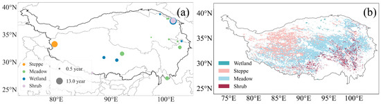
Figure 1.
Spatial distribution of eddy covariance sites and major ecosystem types on the QTP. (a) Locations of eddy covariance sites grouped by plant functional type, together with their observation durations. Circles indicate site locations, with different colors representing vegetation types. Circle size denotes the length of the time series, with larger circles corresponding to longer observation periods. (b) Spatial distribution of dominant ecosystem types, including alpine meadow, alpine steppe, wetland, and shrub.
2.2. Data Description
2.2.1. Eddy Covariance Data
In this study, we collected eddy covariance (EC) flux data across the QTP. For sites with discontinuous temporal records, the data were divided into two or more sub-sites based on time intervals to ensure continuity in the time series. As a result, the original 19 site records were expanded to 29 site records (Table S1). The NamCo site data were sourced from [23], which provided half-hourly net ecosystem exchange measurements along with corresponding environmental variables. To derive GPP estimates, the raw EC flux data were processed using the REddyProc R package (version 1.3.2), a widely used post-processing tool developed by the Max Planck Institute for Biogeochemistry. The processing workflow included u* filtering to exclude periods of low turbulence, with the u* threshold estimated via the Moving Point Test and seasoning restricted to the same months within each year. NEE gap-filling was performed using lookup tables and mean diurnal courses [24]. Flux partitioning into GPP and ecosystem respiration was conducted using the nighttime-based method [24]. Site-specific metadata were supplied during processing to ensure accuracy. Other data were obtained from [25] and the “20th Anniversary Dataset of ChinaFLUX” published by the National Ecosystem Science Data Center (https://nesdc.org.cn/collection/view/64ed74067e2817429fbc7ceb, accessed on 20 January 2024) [5].
The spatial distribution of the flux sites is shown in Figure 1a. The dataset includes 9 alpine meadow sites, 1 alpine steppe sites, 6 wetland sites, and 3 shrub sites, mainly concentrated in the eastern and southeastern parts of the QTP. To ensure consistency in data processing, all flux measurements were aggregated to a monthly temporal resolution. Specifically, daily GPP values were averaged to obtain monthly GPP, which served as the response variable for subsequent modeling and analysis.
2.2.2. Geospatial Data
The predictor variables used for GPP estimation in this study include air temperature (TA), atmospheric pressure (pres), wind speed (wind), surface downward shortwave radiation (srad), precipitation rate, normalized difference vegetation index, enhanced vegetation index (EVI), soil water content (SW), soil temperature (Ts), solar-induced chlorophyll fluorescence (SIF), leaf area index (LAI), fraction of absorbed photosynthetically active radiation (FAPAR), and vapor pressure deficit (VPD), as detailed in Table 1. Land cover data were used to identify the spatial distribution of ecosystem types across the QTP for subsequent upscaling procedures [26].

Table 1.
Description of input variables for GPP modeling.
To facilitate subsequent upscaling, all input variables were first clipped to the spatial extent of the QTP. To ensure consistency across datasets, these variables were then resampled to a uniform spatial resolution of 0.05° using the nearest neighbor method and aggregated to a monthly temporal scale. During model training, pixel-level values corresponding to each flux site were extracted to construct the training dataset.
2.2.3. Overview of Benchmark GPP Products
FLUXCOM X-base [21], FluxSat [19], and GOSIF [20] served as the three benchmark GPP products for comparison in this study. FLUXCOM X-base upscales site-level flux observations from the FLUXNET network to global scale using machine learning methods, primarily driven by MODIS vegetation indices and radiation-related variables. FluxSat employs a simplified LUE framework, with MODIS optical remote sensing data as the main input, and model parameters calibrated against flux tower measurements, making it a data-driven GPP product. GOSIF derives GPP estimates by establishing empirical relationships between SIF and GPP at flux sites, with SIF retrieved from the GOSIF product.
2.3. Methods
2.3.1. AutoML Platforms
AutoML is a technique that automates the entire ML pipeline, including feature selection, model algorithm selection, and hyperparameter tuning. It significantly improves modeling efficiency and reduces the need for manual intervention [34]. Compared to traditional model ensemble techniques and hyperparameter tuning methods, AutoML offers enhanced reproducibility and adaptability while maintaining high model performance, making it particularly suitable for complex ecosystem modeling tasks. In this study, we employed two representative AutoML platforms, H2O AutoML and FLAML, which, respectively, exemplify comprehensive and lightweight AutoML strategies. The specific algorithms and their characteristics are summarized in Table S2.
The H2O AutoML platform, created by H2O.ai, streamlines ML workflows by automating model construction and hyperparameter optimization [35]. It supports a wide range of model families and automatically selects the top-performing algorithms. By employing stacked ensemble techniques and randomized hyperparameter search, H2O AutoML effectively balances model diversity, predictive accuracy, and computational efficiency. FLAML provides a lightweight and efficient AutoML approach. It uses cost-effective models and fast hyperparameter tuning [17]. Unlike many frameworks, it does not rely on ensemble or meta-learning. This makes model training faster and more resource-friendly. FLAML also supports automatic hyperparameter optimization by minimizing loss functions (e.g., log loss or mean squared error) under user-defined constraints [18].
2.3.2. Model Development
The in-situ observations were classified into four ecosystem types based on PFTs. For each PFT, the dataset was randomly split into training (80%) and testing (20%) subsets using the train_test_split function from scikit-learn, with a fixed random seed to ensure reproducibility and robustness of the partitioning. During model training, two automated machine learning platforms—H2O AutoML and FLAML—were employed. For H2O AutoML, mean squared error (MSE) served as the loss function. An internal validation set was derived from the training data to evaluate the performance of individual base learners and to construct stacked ensemble models, thereby enhancing prediction stability and generalization capability. For FLAML, MSE was similarly used as the optimization objective, leveraging its built-in automated hyperparameter tuning and model selection mechanisms to efficiently screen and optimize a diverse set of machine learning algorithms.
Model performance was comprehensively evaluated on both the training and independent testing sets using metrics including the coefficient of determination (R2), root mean squared error (RMSE), and mean absolute error. The best-performing model for each PFT was ultimately selected for subsequent regional-scale GPP upscaling. At the regional scale, land cover data were used to identify the spatial distribution of pixels belonging to the four ecosystem types. The gridded values of all predictor variables were then fed into the trained models to estimate GPP across the QTP. The detailed workflow is shown in Figure 2.
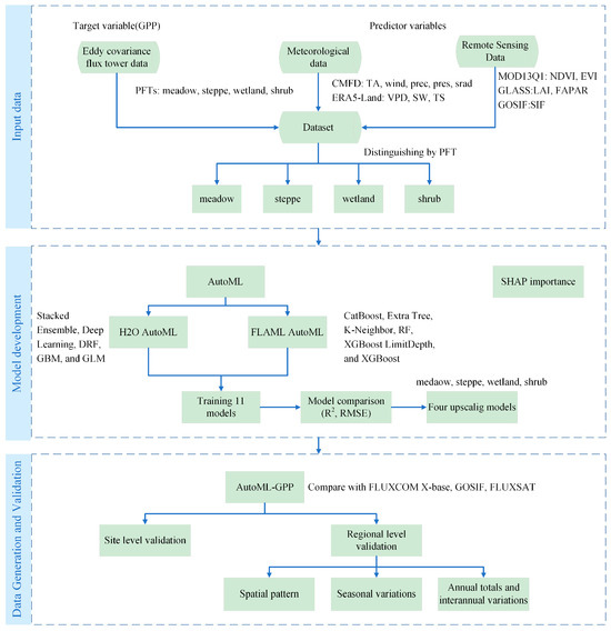
Figure 2.
Workflow for GPP estimation, model optimization, and validation across different plant functional types (PFTs). First, the input variables required for modeling are prepared, including meteorological variables and other environmental factors, along with the target variable GPP. Subsequently, two AutoML platforms—H2O AutoML and FLAML AutoML—are employed to construct models for different vegetation types using multiple machine learning algorithms. For each PFT, the best-performing model is selected for subsequent spatial upscaling. Finally, a GPP dataset for the QTP is generated, and its spatial distribution patterns and interannual variability are further analyzed.
2.3.3. Feature Importance Analysis Using SHAP
We employed the Shapley (SHAP) method to better understand the relationships between GPP and other predictor variables, and to identify the most influential features as well as how each contributes to the model’s predictions. SHAP, grounded in cooperative game theory, assigns an importance value to each input variable based on its marginal contribution to the prediction, enabling interpretability of complex machine learning models [25]. Compared to traditional feature importance techniques, SHAP maintains model performance while offering consistency, local interpretability, and a unified framework, making it widely adopted in ecological and environmental studies [18,36].
In this study, we used XGBoost (version 3.1.2) to compute feature attributions for the four major PFTs: alpine meadow, alpine steppe, wetland, and shrub. For each PFT, we calculated the mean absolute SHAP values of all predictor variables to assess their relative contributions to GPP prediction. In addition to quantifying global feature importance, SHAP also reveals the heterogeneity of variable effects across different PFTs.
3. Results
3.1. Site-Level Evaluation of AutoML-GPP and Other Data-Driven GPP Products
3.1.1. Performance of the AutoML-GPP Model at the Site Level
Figure 3 illustrates the site-level performance of the optimal machine learning models in estimating GPP across different ecosystem types. Overall, the predicted GPP values showed strong agreement with flux tower observations, though performance varied somewhat among ecosystems.
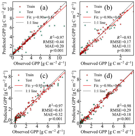
Figure 3.
Site-level GPP predictions using the optimal machine learning algorithm for each ecosystem type: (a) alpine meadow—Stacked Ensemble; (b) alpine steppe—Random Forest; (c) shrub—XGBoost; and (d) wetland—Stacked Ensemble.
For the meadow site, the Stacked Ensemble model exhibited excellent performance (Figure 3a; R2 = 0.97, RMSE = 0.44 g C m−2 d−1). At the steppe site, the Random Forest model yielded robust results, with R2 = 0.93, and RMSE = 0.17 g C m−2 d−1 (Figure 3b). The shrub site, modeled using XGBoost, also demonstrated high accuracy (R2 = 0.97; RMSE = 0.43 g C m−2 d−1; Figure 3c), effectively capturing the observed variability in GPP. For the wetland site, the Stacked Ensemble model again performed best, with R2 = 0.98 and RMSE = 0.29 g C m−2 d−1 (Figure 3d), indicating strong predictive capability across temporal variations. Detailed performance metrics for each ecosystem type and model are provided in Tables S3–S6.
3.1.2. Site-Level Comparative Evaluation of Model Performance with Other Data-Driven GPP Products
To ensure a fair comparison, we used the same in situ data as in the model training stage to consistently extract regional-scale values of AutoML-GPP and three widely used GPP products (FLUXCOM X-base, FluxSat, and GOSIF), and subsequently analyzed their site-level performance. Figure 4 shows a comparison of GPP products across various ecosystem types on the QTP, evaluated against flux tower observations. The results indicate that AutoML-GPP consistently outperforms FLUXCOM X-base, FluxSat, and GOSIF in alpine meadow and shrub ecosystems. While AutoML-GPP does not yield the highest median R2 in wetland areas, it records the lowest median RMSE, indicating greater stability and accuracy in predictions for this ecosystem type (AutoML: median R2 = −0.17, median RMSE = 1.56 g C m−2 d−1, FLUXCOM X-base: median R2 = 0, median RMSE = 1.90 g C m−2 d−1, FluxSat: median R2 = 0.26, median RMSE = 1.80 g C m−2 d−1, GOSIF: median R2 = −0.93, median RMSE = 2.80 g C m−2 d−1). Specifically, AutoML-GPP exhibits higher and more consistent R2 values with smaller interquartile ranges, reflecting enhanced model stability and generalization across flux sites. For instance, in alpine meadow and shrub, AutoML-GPP delivers the highest median R2 values and the tightest interquartile ranges, underscoring its robust performance across diverse sites (AutoML: (meadow) median R2 = 0.82, (shrub) median R2 = 0.69, FLUXCOM X-base: median R2 = 0.60, (shrub) median R2 = 0.02, FluxSat: median R2 = 0.60, (shrub) median R2 = 0.30, GOSIF: median R2 = 0.39, (shrub) median R2 = −0.82). Additionally, AutoML-GPP consistently achieves lower RMSE values, indicating superior fitting accuracy. To further evaluate model performance, we extracted site-level GPP values from the regional GPP datasets and conducted scatterplot comparisons. The results still demonstrate superior performance of AutoML-GPP (Figure S1).
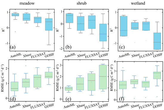
Figure 4.
Comparative evaluation of model performance for AutoML, FLUXCOM X-base, FluxSat, and GOSIF at individual flux sites across three ecosystem types. Boxplots of R2 and RMSE for different GPP products across meadow, shrub, and wetland ecosystems: (a) R2 for meadow sites; (b) R2 for shrub sites; (c) R2 for wetland sites; (d) RMSE for meadow sites; (e) RMSE for shrub sites; (f) RMSE for wetland sites. Since only a single flux site was available for the steppe ecosystem, a boxplot was not displayed. Boxplots of R2 and RMSE for different GPP products across meadow, shrub, and wetland ecosystems. Boxes represent the interquartile range (25th–75th percentiles), the central line indicates the median (50th percentile), whiskers extend to 1.5× interquartile range, and individual points denote outliers.
3.1.3. SHAP-Based Interpretation of Feature Importance Across PFTs
Feature importance in GPP prediction across different ecosystem types was further examined using the SHAP method (Figure 5). The results reveal marked ecosystem-specific differences in the relative contributions of climatic and vegetation-related variables, reflecting distinct mechanisms controlling GPP in each ecosystem type.
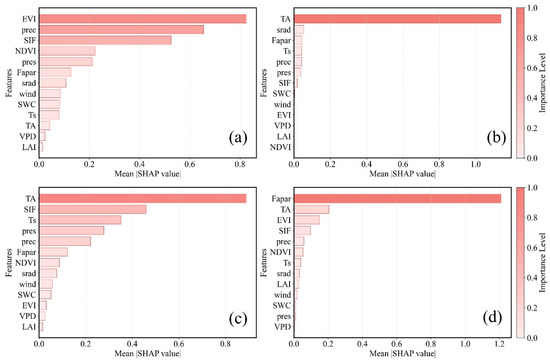
Figure 5.
SHAP importance plots for four vegetation types: (a) Alpine Meadow, (b) Alpine Steppe, (c) Wetland, (d) Shrub.
In alpine meadow ecosystems, EVI emerged as the dominant predictor, highlighting the pivotal role of vegetation growth and canopy development in regulating GPP under relatively favorable moisture and temperature conditions. By contrast, TA exerted the strongest influence in alpine steppe and wetland ecosystems, indicating pronounced energy limitations driven by freeze–thaw cycles and low thermal availability that constrain photosynthetic activity. In shrub ecosystems, FAPAR ranked highest in importance, underscoring the critical contribution of radiation absorption efficiency and canopy structure to GPP dynamics.
Overall, these findings illustrate a shift in GPP controls across the QTP from vegetation-driven processes in more productive ecosystems to temperature-constrained mechanisms in colder, sparsely vegetated systems. This pattern underscores the value of ecosystem-specific modeling approaches.
3.2. Spatiotemporal Dynamics of GPP: Evaluation and Interpretation
3.2.1. Spatial Pattern
Figure 6 shows the seasonal spatial distribution patterns of AutoML-GPP across the QTP. In spring and winter, the overall GPP decreases, while the proportion of pixels with GPP values in the 0–1 g C m−2 d−1 range increases. In contrast, during summer and autumn, GPP increases markedly as vegetation becomes greener, reflecting enhanced photosynthetic activity and an increased proportion of pixels with high GPP values. Spatially, the eastern alpine meadow regions exhibit higher GPP values compared with the western alpine steppe region. Figure 7 shows the spatial distribution of GPP derived from different products across the study area. Overall, all products exhibit a high degree of consistency in spatial patterns, showing a clear decreasing trend from southeast to northwest, with significantly higher GPP values in the eastern regions compared to the west. High GPP values are mainly distributed in the alpine meadow areas of the east, while the western alpine steppe regions show relatively lower GPP values. The high-value areas of the AutoML-GPP are relatively smaller than those in FLUXCOM X-base, FluxSat, and GOSIF, while showing higher GPP estimates in the western alpine steppe regions. Due to missing pixel-level GPP values in the other three products, particularly in the FluxSat product, their spatial patterns of GPP are not entirely consistent. In contrast, AutoML-GPP provides more complete spatial coverage, offering a more comprehensive depiction of GPP spatial patterns across the QTP. The frequency histograms show that most pixels are concentrated in the lower GPP range (0–1 g C m−2 d−1), though certain differences exist among the products. The GOSIF product displays a larger number of high-value pixels (3–5 g C m−2 d−1). Overall, despite numerical discrepancies among the products, their spatial distribution patterns are generally consistent. Moreover, AutoML-GPP exhibits good seasonal and spatial correlations with SIF (Figure S2).
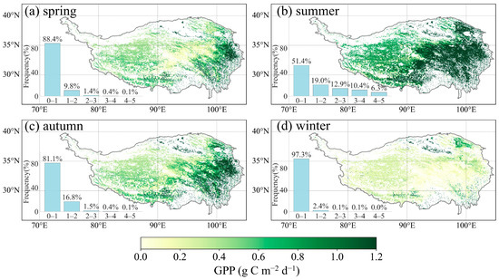
Figure 6.
Spatial patterns and multi-year (2002–2018) mean GPP across the QTP, along with corresponding frequency distributions. The frequency histograms in the subfigures illustrate the distribution of pixels across different GPP values, with the X-axis representing GPP (g C m−2 d−1). Panels: (a) spring, (b) summer, (c) autumn, and (d) winter.
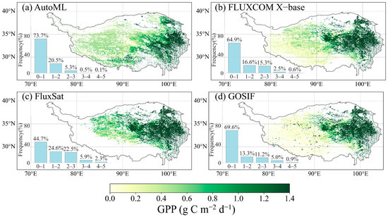
Figure 7.
Spatial patterns and frequency distributions of multi-year mean (2002–2018) GPP across the QTP. (a) AutoML, (b) FLUXCOM X-base, (c) FluxSat, and (d) GOSIF. The frequency histograms in the subfigures illustrate the distribution of pixels across different GPP values, with the X-axis representing GPP (g C m−2 d−1).
3.2.2. Seasonal Cycle of GPP
We examined the seasonal variations in GPP across different ecosystem types and compared our results with three other products (Figure 8). All four GPP products exhibit similar seasonal patterns, with GPP values peaking in July and being substantially higher during the growing season than in the non-growing season. Among the ecosystem types, alpine meadows show the highest GPP and the most pronounced seasonal amplitude, indicating strong photosynthetic activity during the growing season. Shrub and alpine steppes have moderate GPP levels with smaller seasonal fluctuations, whereas wetlands maintain consistently low GPP values throughout the year. AutoML-GPP also shows good consistency and strong correlation with SIF (Figure S2).
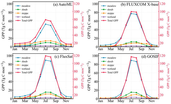
Figure 8.
Seasonal variations in GPP across different ecosystem types derived from four GPP products, representing the multi-year mean during 2002–2018: (a) AutoML-GPP, (b) FLUXCOM X-base, (c) FluxSat, and (d) GOSIF. The left Y-axis represents the GPP of each ecosystem type, while the right Y-axis indicates the total GPP. The blue line denotes the variation in GPP in alpine meadows, the green line represents shrubs, the orange line represents alpine steppes, the purple line indicates wetlands, and the red line shows the variation in total GPP across the four ecosystem types.
3.2.3. Annual Totals and Interannual Variations in GPP
We compared the interannual mean GPP derived from our upscaled AutoML-GPP product with three benchmark products (FLUXCOM X-base, FluxSat, and GOSIF) across different ecosystem types (Figure 9a). The results indicate that AutoML-GPP yielded lower estimates for alpine meadows and higher estimates for alpine steppe compared to the other three products, with corresponding values of 197.42 Tg C yr−1 and 98.15 Tg C yr−1, respectively. To further evaluate the responsiveness of the AutoML-GPP estimate to interannual dynamics of vegetation carbon assimilation over long temporal scales, we analyzed the interannual variations in GPP during 2002–2018 as well as the GPP anomalies (Figure 9b and Figure S3). All four estimates exhibit some degree of interannual anomalies, though their magnitudes vary substantially. AutoML-GPP estimates total annual GPP ranging from 356.30 to 393.90 Tg C yr−1, and a multi-year mean of 374.20 Tg C yr−1. It exhibits a slight increasing trend with a slope of 0.08 Tg C yr−1. In comparison, FluxSat estimates significantly higher mean annual GPP (483.94 Tg C yr−1), along with a much stronger increasing trend (1.30 Tg C yr−1). GOSIF also exhibits a pronounced increasing trend (1.27 Tg C yr−1). Notably, FLUXCOM X-base shows a slight decreasing trend (−0.56 Tg C yr−1), which is opposite to the increasing trends observed in the other three GPP products and SIF, suggesting that the FLUXCOM X-base result may be less reliable in capturing the long-term GPP dynamics over the QTP.
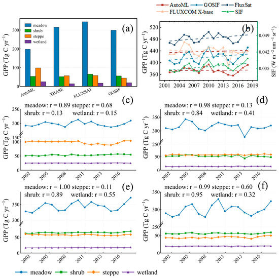
Figure 9.
(a) Mean GPP values across different ecosystem types from 2002 to 2018 for each product. (b) Interannual variations in total GPP over the QTP. Dashed lines indicate the fitted linear trends, with colors corresponding to the respective GPP products shown by the solid lines. The fitted regression equations and significance levels (p-values) for total GPP and SIF are as follows: AutoML, Y = 0.08x + 205.09, p = 0.881; GOSIF, Y = 1.27x + 2142.27, p = 0.173; FluxSat, Y = 1.30x − 2131.39, p = 0.096; FLUXCOM X-base, Y = −0.56x + 1567.00, p = 0.535; and SIF, Y = 0.0002x − 0.32, p = 0.033. (c–f) Interannual variations in GPP for different ecosystem types across the QTP and the Pearson correlation coefficients between each ecosystem type and total GPP for the four products: (c) AutoML, (d) FLUXCOM X-base, (e) FluxSat, and (f) GOSIF.
We further analyzed the contributions of different ecosystem types to the regional total GPP and compared the results among the four GPP products (Figure 9c–f). The results indicate that alpine meadow not only contributes the largest share to total GPP but also exhibits the strongest correlation with it (AutoML: r = 0.89, FLUXCOM X-base: r = 0.98, FluxSat: r = 1.00, GOSIF: r = 0.99), highlighting its role as the dominant ecosystem type driving interannual GPP variability across the QTP. In contrast, wetlands contribute the least, with annual GPP emissions considerably lower than those of alpine meadow, alpine steppe, and shrubland. Notably, the relative contribution of alpine steppes varied among products. The upscaled results from this study (AutoML-GPP) suggest that alpine steppes represent the second-largest contributor to total GPP after alpine meadows, while in the other three products, the annual GPP of alpine steppes is lower than that in shrub. Given that alpine steppes are the dominant ecosystem type on the QTP, with an area far larger than that of shrub, the higher GPP estimated for alpine steppes in this study appears more reasonable. Spatially, the GPP trends derived from AutoML-GPP were generally consistent with those from FLUXCOM X-base. However, AutoML-GPP revealed a more extensive area of GPP decline across the alpine steppe. The FluxSat product showed decreasing GPP primarily over the western alpine steppe, whereas GOSIF indicated a weakening trend mainly in limited portions of the alpine meadow and alpine steppe regions (Figure S4).
To quantify the interannual dynamics, GPP anomalies were calculated as the difference between the annual GPP and the mean GPP during 2002–2018. The years 2008, 2010, and 2015 showed the greatest interannual variability, among which 2010 exhibited the most pronounced positive anomaly, with GPP exceeding the average by approximately 19.70 Tg C yr−1 (Figure 9b and Figure S3). In contrast, 2008 showed the strongest negative anomaly (9.40 Tg C yr−1). Another noticeable dropdown occurred in 2015, likely associated with climate anomalies triggered by the 2015/2016 strong El Niño event. Comparison with the remaining GPP products indicates that these key years consistently exhibited similar anomaly peaks or troughs across various estimates, suggesting a coherent response of regional carbon uptake to large-scale climatic perturbations. However, the FLUXCOM X-base displayed a sharp drop in GPP in 2014, followed by a rapid rebound in 2015, deviating from the patterns seen in the other products (Figure 9b).
Figure 10 illustrates the seasonal anomalies of GPP in 2008, 2010, and 2015 derived from different products. Overall, the four products capture the temporal and spatial variations in GPP reasonably well (Figure 10 and Figure S5). However, the FLUXCOM X-base product shows a noticeable inconsistency with the others in 2015 (Figure 10f). Specifically, its GPP increase from January to July is greater than the decrease from August to December, which is opposite to the overall trend observed in the other products and thus fails to effectively represent the abnormal GPP variation that year. The decrease in GPP in 2008 (Figure 10a), as observed in AutoML-GPP and the three benchmark products, coincided with a decline in soil temperature during July–September, despite an increase in soil moisture over the same period (Figures S6g,j and S7g,j). In contrast, the significant decrease in GPP during July–September of 2015 (Figure 10c) was primarily caused by the El Niño event, which led to reductions in both soil temperature and soil moisture (Figures S6i,l and S7i,l).
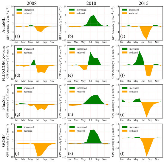
Figure 10.
Seasonal anomalies of GPP over the QTP in years 2008, 2010, and 2015: (a–c) AutoML, (d–f) FLUXCOM X-base, (g–i) FluxSat, and (j–l) GOSIF. Seasonal anomalies were calculated as the difference between the seasonal GPP of a given year and the multi-year seasonal mean during 2002–2018.
4. Discussion
4.1. Main Advantages of AutoML-GPP
Most current data-driven GPP products, such as FLUXCOM X-base, FluxSat, and GOSIF, primarily rely on training data from the FLUXNET 2015 dataset [19,20,21]. However, these training processes rarely incorporate EC observations from the QTP, resulting in limited representation of the region’s unique ecosystem carbon flux characteristics. Additionally, the long-term records in FLUXNET 2015 mainly span from the early 1990s to 2014 [37], which may not sufficiently reflect contemporary ecosystem responses under accelerating global climate change. To overcome these limitations, this study employs the most comprehensive EC observation dataset available from the QTP to develop the AutoML-GPP product. By encompassing four major alpine ecosystem types and integrating data from the most recent years, the dataset substantially enhances the representativeness and generalizability of the model across the region.
To effectively capture the nonlinear relationships between GPP and a diverse set of remote sensing and meteorological drivers, we employed an AutoML approach using two platforms (H2O AutoML and FLAML) to systematically train and evaluate 11 mainstream machine learning algorithms. This strategy facilitates automated selection of optimal model architectures and hyperparameters, mitigating biases associated with single-model approaches and significantly improving predictive accuracy and reproducibility [18]. Additionally, we incorporated 13 eco-meteorological variables as input features, enhancing the model’s ability to characterize the complex processes driving GPP. A PFT-based modeling framework was employed, whereby separate models were constructed for each PFT during the upscaling process [38,39]. This stratified approach better captures the distinct ecophysiological responses and functional traits of individual ecosystem types, thereby enhancing the representation of spatial heterogeneity and ecological realism in regional GPP estimates. Validation against local EC sites indicated that AutoML-GPP surpasses FLUXCOM X-base, FluxSat, and GOSIF in alpine meadow and shrubland ecosystems. These findings underscore the model’s robustness across most QTP ecosystems and highlight areas where data limitations constrain performance.
4.2. Uncertainty in GPP Estimation for the QTP
The EC technique enables continuous, ecosystem-scale monitoring of carbon fluxes [40]. It is widely utilized in ground-based measurements and for validating upscaling models [41]. While EC data are critical for carbon cycle research, their application in constructing and evaluating GPP products introduces several uncertainties, particularly on the QTP, where complex terrain and extreme climatic conditions exacerbate these challenges.
A primary source of uncertainty stems from the limited amount of EC flux towers on the QTP, attributed to harsh environmental conditions, logistical constraints, and high maintenance costs at high altitudes. Available EC time series are often short, discontinuous, and spatially sparse [42]. The temporal distribution of EC tower data used in this study reveals insufficient long-term observations across the four major ecosystem types. This limitation is most pronounced in alpine steppe ecosystems, which dominate the western QTP. Although we considered incorporating data from two additional steppe sites (Ali and Muztag), each providing only one year of observations, their inclusion substantially degraded overall model performance. This degradation likely stems from substantial inter-site differences that the current driving variables fail to adequately capture, reflecting underlying environmental heterogeneity. To enhance the stability and reliability of GPP estimates in alpine steppe regions, we ultimately employed only the long-term, continuous observations from the NamCo site for upscaling.
This region’s harsh environmental conditions and limited infrastructure hinder stable, long-term flux observations, restricting the model’s ability to accurately capture seasonal and interannual GPP dynamics in alpine steppe ecosystems. Consequently, this constraint reduces the generalization capacity and predictive accuracy of data-driven models, leading to considerable uncertainties in steppe GPP predictions. Additionally, the spatial imbalance in EC site distribution exacerbates these uncertainties, with flux towers concentrated primarily in the central and eastern QTP, leaving the western regions significantly underrepresented.
When the regional GPP product was evaluated against site-level observations, performance was noticeably poorer for wetland ecosystems (Figure 4). This discrepancy is primarily attributable to the substantial uncertainty in wetland classification across the QTP. First, wetland definitions and classification criteria remain inconsistent across studies [43]. Second, the complex topography, frequent cloud cover and extensive permafrost considerably complicate remote sensing-based classification. Seasonal and interannual dynamics of wetlands further exacerbate classification errors. Moreover, the harsh environmental conditions severely limit the availability of ground-truth validation data. Collectively, these factors result in large disparities in estimated wetland area on the QTP, ranging from 3.76 × 10⁴ to 87.5 × 10⁴ km2 across studies [35]. Consequently, future efforts should prioritize the establishment of additional wetland flux towers and the development of higher-resolution, more accurate wetland distribution maps to substantially improve the reliability and precision of regional GPP estimates in these ecosystems.
In addition, meteorological forcing datasets represent another source of uncertainty. At the regional scale, carbon cycle modeling relies heavily on gridded meteorological forcing datasets. However, the limited number and uneven spatial distribution of meteorological observation stations often lead to substantial discrepancies in the spatiotemporal consistency and accuracy of these datasets, which are typically generated through various spatial interpolation techniques [44,45]. These uncertainties are particularly pronounced in high-altitude regions such as the QTP, where complex climatic conditions and sparse observational coverage exacerbate errors in meteorological drivers. Biases in key forcing variables, such as temperature, precipitation, and solar radiation, can significantly compromise the accuracy and reliability of GPP estimates.
5. Conclusions
Leveraging recent advancements in ground-based eddy covariance flux observations and multi-source remote sensing data, this study developed a high spatiotemporal resolution GPP dataset for the QTP using state-of-the-art automated machine learning (AutoML) techniques. By evaluating 11 machine learning algorithms and selecting the best-performing model for each PFT, we systematically assessed the spatiotemporal patterns of carbon assimilation and its climatic drivers across the region. The main findings are summarized as follows:
- (1)
- Validation against in situ flux observations at the site scale indicates that the model performs robustly across alpine meadow, alpine steppe, wetland, and shrub ecosystems, achieving R2 values up to 0.95 and RMSE as low as 0.42 g C m−2 d−1 in the testing set. By validating extracted site-level GPP values from the upscaling GPP datasets against flux observations, AutoML-GPP demonstrates overall superior or equivalent performance over global GPP products (FLUXCOM X-base, GOSIF, and FluxSat).
- (2)
- AutoML-GPP effectively captures the spatiotemporal variability of GPP over the QTP. During 2002–2018, the mean annual GPP was approximately 374.20 Tg C yr−1, exhibiting a slight increasing trend of about 0.08 Tg C yr−1. Spatially, GPP is higher in the eastern QTP, dominated by alpine meadows, and lower in the west, dominated by alpine steppes, reflecting the strong influence of hydrothermal conditions and ecosystem type on regional carbon uptake capacity.
- (3)
- Notable interannual GPP anomalies due to climate extremes were identified in the years 2008, 2010, and 2015, with spatiotemporal patterns closely coinciding with anomalies in meteorological variables. AutoML-GPP estimates a similar annual mean magnitude of GPP but more reasonable interannual anomalies than the recent released well-known global upscaling flux dataset FLUXCOM X-base.
In conclusion, the AutoML-GPP product delivers a regionally tailored and ecologically coherent estimation of GPP for the QTP. As a valuable complement to existing products, it provides a robust data foundation for carbon budget assessments and research on ecosystem–climate interactions in high-altitude environments.
Supplementary Materials
The following supporting information can be downloaded at: https://www.mdpi.com/article/10.3390/rs18010130/s1, Figure S1: Site-level scatter plots comparing observed and estimated GPP across different plant functional types (PFTs) for AutoML-GPP and three benchmark products (FLUXCOM X-base, GOSIF, and FluxSat). The dashed line represents the 1:1 reference line, and the solid line indicates the linear regression fit. Scatter points are color-coded by the magnitude of observed GPP values (varying along the x-axis) to visually highlight the gradient and distribution of observed GPP across different ranges. (a–d) alpine meadow, (e–h) shrubland, (i–l) wetland, and (m–o) alpine steppe. For all products, including AutoML-GPP, estimated GPP values were extracted directly from the gridded regional products at the exact pixel locations corresponding to the flux sites, and then compared against in-situ measurements to ensure a fair and consistent evaluation. Note that FluxSat data were unavailable for alpine steppe due to extensive data gaps over the western QTP, resulting in no valid matching records at the flux sites; Figure S2: Monthly variation and spatial correlation between GPP and SIF (based on multi-year monthly averages) from different products over the QTP during 2002–2018. SIF data are derived from GOSIF [32]. (a) Seasonal variations of GPP from different products and SIF. (b) AutoML; (c) FLUXCOM X−base; (d) FluxSat; (e) GOSIF; Figure S3: GPP anomalies for AutoML-GPP. Anomalies were calculated as the difference between the annual GPP estimate and the multi-year mean (2002–2018); Figure S4: Spatial patterns of GPP temporal trends over the QTP during 2002–2018 derived from different products: (a) AutoML, (b) FLUXCOM X−base, (c) FluxSat, and (d) GOSIF; Figure S5: Spatial patterns of GPP anomalies during July–August of the years 2008, 2010, and 2015: (a–c) AutoML, (d–f) FLUXCOM X-base, (g–i) FluxSat, (j–l) GOSIF; Figure S6: (a–c) Interannual anomalies of AutoML-GPP in 2008, 2010, and 2015. Corresponding seasonal anomalies expressed as Z-scores are shown for SIF (d–f), soil water (g–i), and soil temperature (j–l); Figure S7: Spatial patterns of GPP anomalies and z-scores of SIF, Ts and SW for the July–August periods of 2008, 2010, and 2015. (a–c) AutoML-GPP anomalies (ΔGPP); (d–f) Z-scores of SIF; (g–i) Z-scores of Ts; (j–l) Z-scores of SW. GPP anomalies (ΔGPP) were calculated as the difference between the mean value of July and August in each year and the long term mean for July–August over 2002–2018. Z-scores of SIF, Ts and SW were computed as: Z = (P_JA − P_JA_mean)/P_JA_std, where P_JA is the average of July and August in the target year, and P_JA_mean and P_JA_std are the multi-year mean and standard deviation for July–August over 2002–2018; Table S1: Eddy covariance (EC) sites used in this study, comprising a total of 62 site-years. For sites with discontinuous temporal records, the data were divided into two or more sub-sites based on time intervals to ensure continuity in the time series. As a result, the original 19 site records were expanded to 29 site records; Table S2: The ML algorithms in the AutoML platforms used for this study; Table S3: Performance metrics of training and testing sets for alpine meadow: Comparison of AutoML models from the H2O platform (including Stacked Ensemble, Deep Learning, DRF, GBM, and GLM) and FLAML (including CatBoost, Extra Tree, K-Neighbor, RF, XGBoost LimitDepth, and XGBoost); Table S4: Similar to Table S3, but for alpine shrub; Table S5: Similar to Table S3, but for wetland; Table S6: Similar to Table S3, but for alpine steppe. Reference [32] is cited in the Supplementary Materials.
Author Contributions
Conceptualization, M.Z., W.H., H.Y. and P.X.; Methodology, M.Z. and S.L.; Validation, M.Z., G.W., H.Y. and N.T.N.; Formal analysis, M.Z. and W.H.; Resources, J.W.; Data curation, M.Z.; Writing—original draft, M.Z.; Writing—review & editing, Y.Y., G.W., W.H., H.Y., N.T.N., J.W., S.L., J.C., X.L., T.M., Z.H. and P.X.; Visualization, M.Z., W.H., H.Y., N.T.N., S.L. and P.X.; Supervision, W.H. and P.X.; Funding acquisition, W.H. All authors have read and agreed to the published version of the manuscript.
Funding
This research is funded by the Basic Research Program of Qinghai Province (Grant No. 2025-ZJ-737), the Key Project of the Open Research Fund of the Qinghai Provincial Key Laboratory of Greenhouse Gases and Carbon Neutrality (Grant No. ZDXM-2025-2), and the National Natural Science Foundation of China (Grant No. 42277453).
Data Availability Statement
The ERA5-Land data are from the Climate Data Store of the Copernicus Climate Service Center (https://cds.climate.copernicus.eu/datasets/reanalysis-era5-land-monthly-means?tab=overview, accessed on 25 January 2024). The CMFD data are from the National Qinghai–Tibet Plateau Data Center (https://data.tpdc.ac.cn/en/data/8028b944-daaa-4511-8769-965612652c49, accessed on 25 January 2024). The GLASS LAI and FAPAR products are available at https://glass.hku.hk/download.html (accessed on 26 January 2024). GOSIF is available from https://globalecology.unh.edu/data/GOSIF.html (accessed on 26 January 2024). MODIS NDVI and EVI are from the Google Earth Engine platform. The upscaled flux data were obtained from (https://doi.org/10.3390/rs15112749, accessed on 20 January 2024) and the “20th Anniversary Dataset of ChinaFLUX” published by the National Ecosystem Science Data Center (https://nesdc.org.cn/collection/view/64ed74067e2817429fbc7ceb, accessed on 20 January 2024). The FluxSat data is available from https://daac.ornl.gov/VEGETATION/guides/FluxSat_GPP_FPAR.html (accessed on 27 January 2024). Other GPP products like the FLUXCOM X-base and GOSIF are available from https://doi.org/10.18160/5NZG-JMJE and https://globalecology.unh.edu/data/GOSIF-GPP.html (accessed on 26 June 2025).
Acknowledgments
We acknowledge ChinaFLUX for providing the flux tower data. We sincerely acknowledge Jingfeng Xiao from New Hampshire University for sharing the GOSIF data.
Conflicts of Interest
Author Guoyong Weng was employed by the company Taizhou Huangyan Urban and Rural Water Supply Co., Ltd. The remaining authors declare that the research was conducted in the absence of any commercial or financial relationships that could be construed as a potential conflict of interest.
References
- Beer, C.; Reichstein, M.; Tomelleri, E.; Ciais, P.; Jung, M.; Carvalhais, N.; Rödenbeck, C.; Arain, M.A.; Baldocchi, D.; Bonan, G.B.; et al. Terrestrial gross carbon dioxide uptake: Global distribution and covariation with climate. Science 2010, 329, 834–838. [Google Scholar] [CrossRef]
- Cheng, G.; Zhao, L.; Li, R.; Wu, X.; Sheng, Y.; Hu, G.; Zou, D.; Jin, H.; Li, X.; Wu, Q. Characteristic, changes and impacts of permafrost on Qinghai-Tibet Plateau. Chin. Sci. Bull. 2019, 64, 2783–2795. [Google Scholar] [CrossRef]
- Dong, L.; Wang, X. Inconsistent influence of temperature, precipitation, and CO2 variations on the plateau alpine vegetation carbon flux. Npj Clim. Atmos. Sci. 2025, 8, 91. [Google Scholar] [CrossRef]
- Wang, Y.; Xiao, J.; Ma, Y.; Ding, J.; Chen, X.; Ding, Z.; Luo, Y. Persistent and enhanced carbon sequestration capacity of alpine grasslands on Earth’s Third Pole. Sci. Adv. 2023, 9, eade6875. [Google Scholar] [CrossRef]
- Yu, G.-R.; Chen, Z.; Wang, Y.-P. Carbon, water and energy fluxes of terrestrial ecosystems in China. Agric. For. Meteorol. 2024, 346, 109890. [Google Scholar] [CrossRef]
- Stocker, B.D.; Zscheischler, J.; Keenan, T.F.; Prentice, I.C.; Seneviratne, S.I.; Peñuelas, J. Drought impacts on terrestrial primary production underestimated by satellite monitoring. Nat. Geosci. 2019, 12, 264–270. [Google Scholar] [CrossRef]
- Wang, H.; Jia, G.; Epstein, H.E.; Zhao, H.; Zhang, A. Integrating a PhenoCam-derived vegetation index into a light use efficiency model to estimate daily gross primary production in a semi-arid grassland. Agric. For. Meteorol. 2020, 288, 107983. [Google Scholar] [CrossRef]
- Jiang, C.; Ryu, Y. Multi-scale evaluation of global gross primary productivity and evapotranspiration products derived from Breathing Earth System Simulator (BESS). Remote Sens. Environ. 2016, 186, 528–547. [Google Scholar] [CrossRef]
- He, H.; Liu, M.; Xiao, X.; Ren, X.; Zhang, L.; Sun, X.; Yang, Y.; Li, Y.; Zhao, L.; Shi, P.; et al. Large-scale estimation and uncertainty analysis of gross primary production in Tibetan alpine grasslands. J. Geophys. Res. Biogeosci. 2014, 119, 466–486. [Google Scholar] [CrossRef]
- Li, J.; Jia, K.; Zhao, L.; Tao, G.; Zhao, W.; Liu, Y.; Yao, Y.; Zhang, X. An improved gross primary production model considering atmospheric CO2 fertilization: The Qinghai–Tibet Plateau as a case study. Remote Sens. 2024, 16, 1856. [Google Scholar] [CrossRef]
- Ma, M.; Yuan, W.; Dong, J.; Zhang, F.; Cai, W.; Li, H. Large-scale estimates of gross primary production on the Qinghai-Tibet plateau based on remote sensing data. Int. J. Digit. Earth 2018, 11, 1166–1183. [Google Scholar] [CrossRef]
- Lin, S.; Wang, G.; Feng, J.; Dan, L.; Sun, X.; Hu, Z.; Chen, X.; Xiao, X. A carbon flux assessment driven by environmental factors over the Tibetan Plateau and various permafrost regions. J. Geophys. Res. Biogeosci. 2019, 124, 1132–1147. [Google Scholar] [CrossRef]
- Huang, Y.; Nicholson, D.; Huang, B.; Cassar, N. Global estimates of marine gross primary production based on machine learning upscaling of field observations. Glob. Biogeochem. Cycles 2021, 35, e2020GB006718. [Google Scholar] [CrossRef]
- Liu, S.; He, W.; Xu, P.; Zhao, M.; Huang, C.; Nguyen, N.T. Modeling carbonyl sulfide and carbon dioxide fluxes in a northern boreal coniferous forest using memory-based deep learning. Ecol. Model. 2025, 510, 111283. [Google Scholar] [CrossRef]
- Ma, Y.; Guan, X.; Wang, Y.; Li, Y.; Lin, D.; Shen, H. GPP estimation by transfer learning with combined solar-induced chlorophyll fluorescence and eddy covariance data. Int. J. Appl. Earth Obs. Geoinf. 2025, 139, 104503. [Google Scholar] [CrossRef]
- Jung, M.; Schwalm, C.; Migliavacca, M.; Walther, S.; Camps-Valls, G.; Koirala, S.; Anthoni, P.; Besnard, S.; Bodesheim, P.; Carvalhais, N.; et al. Scaling carbon fluxes from eddy covariance sites to globe: Synthesis and evaluation of the FLUXCOM approach. Biogeosciences 2020, 17, 1343–1365. [Google Scholar] [CrossRef]
- Zheng, Z.; Fiore, A.M.; Westervelt, D.M.; Milly, G.P.; Goldsmith, J.; Karambelas, A.; Curci, G.; Randles, C.A.; Paiva, A.R.; Wang, C.; et al. Automated machine learning to evaluate the information content of tropospheric trace gas columns for fine particle estimates over India: A modeling testbed. J. Adv. Model. Earth Syst. 2023, 15, e2022MS003099. [Google Scholar] [CrossRef]
- Nguyen, N.T.; Lü, H.; He, W.; Xu, P.; Zhao, M.; Liu, S.; Zhu, Y.; Lei, X. Automated machine learning integrating multi-source satellite observations to predict gross and net CO2 fluxes of coastal wetlands in China. Environ. Res. Lett. 2025, 20, 084011. [Google Scholar] [CrossRef]
- Joiner, J.; Yoshida, Y.; Zhang, Y.; Duveiller, G.; Jung, M.; Lyapustin, A.; Wang, Y.; Tucker, C.J. Estimation of terrestrial global gross primary production (GPP) with satellite data-driven models and eddy covariance flux data. Remote Sens. 2018, 10, 1346. [Google Scholar] [CrossRef]
- Li, X.; Xiao, J. Mapping photosynthesis solely from solar-induced chlorophyll fluorescence: A global, fine-resolution dataset of gross primary production derived from OCO-2. Remote Sens. 2019, 11, 2563. [Google Scholar] [CrossRef]
- Nelson, J.A.; Walther, S.; Gans, F.; Kraft, B.; Weber, U.; Novick, K.; Buchmann, N.; Migliavacca, M.; Wohlfahrt, G.; Šigut, L.; et al. X-BASE: The first terrestrial carbon and water flux products from an extended data-driven scaling framework, FLUXCOM-X. Biogeosciences 2024, 21, 5079–5115. [Google Scholar] [CrossRef]
- Tan, K.; Ciais, P.; Piao, S.; Wu, X.; Tang, Y.; Vuichard, N.; Liang, S.; Fang, J. Application of the ORCHIDEE global vegetation model to evaluate biomass and soil carbon stocks of Qinghai-Tibetan grasslands. Glob. Biogeochem. Cycles 2010, 24. [Google Scholar] [CrossRef]
- Nieberding, F.; Wille, C.; Fratini, G.; Asmussen, M.O.; Wang, Y.; Ma, Y.; Sachs, T. A long-term (2005–2019) eddy covariance data set of CO2 and H2O fluxes from the Tibetan alpine steppe. Earth Syst. Sci. Data 2020, 12, 2705–2724. [Google Scholar] [CrossRef]
- Reichstein, M.; Falge, E.; Baldocchi, D.; Papale, D.; Aubinet, M.; Berbigier, P.; Bernhofer, C.; Buchmann, N.; Gilmanov, T.; Granier, A.; et al. On the separation of net ecosystem exchange into assimilation and ecosystem respiration: Review and improved algorithm. Glob. Change Biol. 2005, 11, 1424–1439. [Google Scholar] [CrossRef]
- Lundberg, S.M.; Lee, S.-I. A unified approach to interpreting model predictions. In Proceedings of the 31st Conference on Neural Information Processing Systems (NIPS 2017), Long Beach, CA, USA, 4–9 December 2017; Volume 30, pp. 4765–4774. [Google Scholar]
- Zhou, G.; Ren, H.; Liu, T.; Zhou, L.; Ji, Y.; Song, X.; Lv, X. A new regional vegetation mapping method based on terrain-climate-remote sensing and its application on the Qinghai-Xizang Plateau. Sci. China Earth Sci. 2022, 66, 237–246. [Google Scholar] [CrossRef]
- He, J.; Yang, K.; Tang, W.; Lu, H.; Qin, J.; Chen, Y.; Li, X. The first high-resolution meteorological forcing dataset for land process studies over China. Sci. Data 2020, 7, 25. [Google Scholar] [CrossRef]
- Muñoz Sabater, J. ERA5-Land Monthly Averaged Data from 1950 to Present. Copernicus Climate Change Service (C3S) Climate Data Store (CDS) 2019. Available online: https://cds.climate.copernicus.eu (accessed on 20 December 2024).
- Takaku, J.; Tadono, T.; Doutsu, M.; Ohgushi, F.; Kai, H. Updates of ‘AW3D30’ ALOS global digital surface model with other open access datasets. Int. Arch. Photogramm. Remote Sens. Spatial Inf. Sci. 2020, XLIII-B4-2020, 183–189. [Google Scholar] [CrossRef]
- Yuan, W.; Zheng, Y.; Piao, S.; Ciais, P.; Lombardozzi, D.; Wang, Y.; Ryu, Y.; Chen, G. Increased atmospheric vapor pressure deficit reduces global vegetation growth. Sci. Adv. 2019, 5, eaax1396. [Google Scholar] [CrossRef] [PubMed]
- Didan, K. MODIS/Terra Vegetation Indices 16-Day L3 Global 250m SIN Grid V061 [Data Set]; NASA EOSDIS Land Processes Distributed Active Archive Center: Sioux Falls, SD, USA, 2021. [Google Scholar] [CrossRef]
- Li, X.; Xiao, J. A global, 0.05-degree product of solar-induced chlorophyll fluorescence derived from OCO-2, MODIS, and reanalysis data. Remote Sens. 2019, 11, 517. [Google Scholar] [CrossRef]
- Liang, S.; Cheng, J.; Jia, K.; Jiang, B.; Liu, Q.; Xiao, Z.; Yao, Y.; Yuan, W.; Zhang, X.; Zhao, X.; et al. The Global Land Surface Satellite (GLASS) product suite. Bull. Am. Meteorol. Soc. 2021, 102, E323–E337. [Google Scholar] [CrossRef]
- Gaber, M.; Kang, Y.; Schurgers, G.; Keenan, T. Using automated machine learning for the upscaling of gross primary productivity. Biogeosciences 2024, 21, 2447–2472. [Google Scholar] [CrossRef]
- Jin, Z.; Zhuang, Q.; He, J.-S.; Zhu, X.; Song, W. Net exchanges of methane and carbon dioxide on the Qinghai-Tibetan Plateau from 1979 to 2100. Environ. Res. Lett. 2015, 10, 085007. [Google Scholar] [CrossRef]
- Yuan, Y.; Guo, W.; Tang, S.; Zhang, J. Effects of patterns of urban green-blue landscape on carbon sequestration using XGBoost-SHAP model. J. Clean. Prod. 2024, 476, 143640. [Google Scholar] [CrossRef]
- Pastorello, G.; Trotta, C.; Canfora, E.; Chu, H.; Christianson, D.; Cheah, Y.W.; Poindexter, C.; Chen, J.; Elbashandy, A.; Humphrey, M.; et al. The FLUXNET2015 dataset and the ONEFlux processing pipeline for eddy covariance data. Sci. Data 2020, 7, 225. [Google Scholar] [CrossRef] [PubMed]
- Guo, R.; Chen, T.; Chen, X.; Yuan, W.; Liu, S.; He, B.; Li, L.; Wang, S.; Hu, T.; Yan, Q.; et al. Estimating global GPP from the plant functional type perspective using a machine learning approach. J. Geophys. Res. Biogeosci. 2023, 128, e2022JG007100. [Google Scholar] [CrossRef]
- Huang, C.; He, W.; Liu, J.; Nguyen, N.T.; Yang, H.; Lv, Y.; Chen, H.; Zhao, M. Exploring the potential of long short-term memory networks for predicting net CO2 exchange across various ecosystems with multi-source data. J. Geophys. Res. Atmos. 2024, 129, e2023JD040418. [Google Scholar] [CrossRef]
- Baldocchi, D.D. How eddy covariance flux measurements have contributed to our understanding of global change biology. Glob. Change Biol. 2020, 26, 242–260. [Google Scholar] [CrossRef] [PubMed]
- Chang, X.; Xing, Y.; Gong, W.; Yang, C.; Guo, Z.; Wang, D.; Wang, J.; Yang, H.; Xue, G.; Yang, S. Evaluating gross primary productivity over 9 ChinaFlux sites based on random forest regression models, remote sensing, and eddy covariance data. Sci. Total Environ. 2023, 875, 162601. [Google Scholar] [CrossRef]
- Zeng, J.; Zhou, T.; Xu, Y.; Lin, Q.; Tan, E.; Zhang, Y.; Wu, X.; Zhang, J.; Liu, X. The fusion of multiple scale data indicates that the carbon sink function of the Qinghai-Tibet Plateau is substantial. Carbon Balance Manag. 2023, 18, 19. [Google Scholar] [CrossRef]
- Zhang, B.; Li, Q.; Jing, Y.; Niu, Z.; Gong, P.; Zhang, D. Alpine wetland distribution patterns and decreasing trends in the Qinghai-Tibetan Plateau. Sci. Bull. 2025, 70, 3509–3511. [Google Scholar] [CrossRef]
- Li, X.; Ma, H.; Ran, Y.; Wang, X.; Zhu, G.; Liu, F.; He, H.; Zhang, Z.; Huang, C. Terrestrial carbon cycle model-data fusion: Progress and challenges. Sci. China Earth Sci. 2021, 64, 1645–1657. [Google Scholar] [CrossRef]
- Wang, J.; Fang, W.; Xu, P.; Li, H.; Chen, D.; Wang, Z.; You, Y.; Rafaniello, C. Satellite evidence for divergent forest responses within close vicinity to climate fluctuations in a complex terrain. Remote Sens. 2023, 15, 2749. [Google Scholar] [CrossRef]


Disclaimer/Publisher’s Note: The statements, opinions and data contained in all publications are solely those of the individual author(s) and contributor(s) and not of MDPI and/or the editor(s). MDPI and/or the editor(s) disclaim responsibility for any injury to people or property resulting from any ideas, methods, instructions or products referred to in the content. |
© 2025 by the authors. Licensee MDPI, Basel, Switzerland. This article is an open access article distributed under the terms and conditions of the Creative Commons Attribution (CC BY) license.