Robust Low-Rank and Spatio–Temporal Regularization Framework for Moving-Vehicle Detection in Satellite Videos

Highlights

What are the main findings?

• A robust TV-RPCA framework is proposed that combines PSSV-based low-rank background modeling, nonconvex ${\mathit{\ell }}_p$ foreground regularization, and spatio–temporal TV regularization for moving-vehicle detection in satellite videos.
• Experiments on the VISO and SkySat datasets demonstrate higher F1 scores and cleaner background reconstruction than classical RPCA variants and state-of-the-art deep learning detectors.

What is the implication of the main finding?

• The proposed method enables reliable vehicle detection under low resolution, local misalignment, and highly dynamic backgrounds, which is crucial for large-scale satellite surveillance and traffic monitoring.
• The low-rank plus spatio–temporal regularization strategy can be extended to other remote sensing video tasks, such as change detection and moving object tracking.

Abstract

Satellite videos are widely applied for large-scale surveillance. Existing low-rank matrix decomposition-based methods produce promising results under simple and stationary backgrounds. However, these methods suffer a severe performance drop on satellite videos with complex and dynamic backgrounds. To address these challenges, we propose a matrix-based total variation regularized robust PCA (TV-RPCA) approach for moving-vehicle detection. Specifically, our TV-RPCA uses the partial sum of singular values to model the low-rank background. Moreover, a ${\mathit{\ell }}_p$ norm and a spatial–temporal TV regularization are adopted to encourage the spatial–temporal continuity of foregrounds. The optimization of our TV-RPCA is carried out using the augmented Lagrangian multiplier framework combined with the alternating direction minimization approach. Comprehensive experiments conducted on SkySat and Jilin-1 video data verify the effectiveness of the proposed approach.

1. Introduction

As a novel earth observation platform, video satellites enable continuous monitoring of designated areas and the acquisition of high–temporal-resolution image sequences. With these advantages, satellite videos have recently been applied to a wide range of tasks, including environmental monitoring [1,2], mineral exploration [3,4], and transportation analysis [5,6]. Among them, moving object detection (MOD), which aims to separate the background and extract moving objects simultaneously, constitutes a fundamental yet challenging problem.

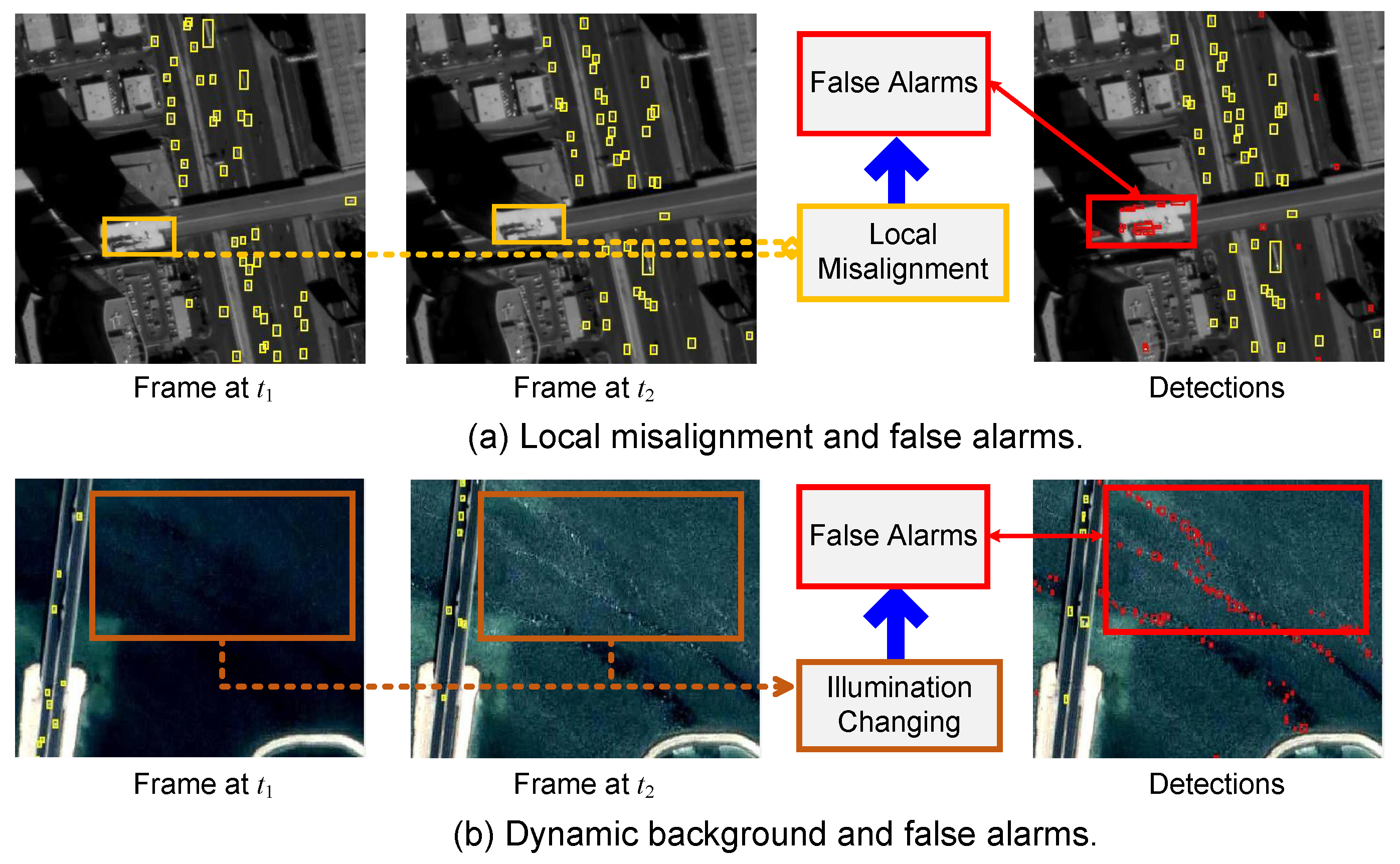
Despite extensive progress achieved in ground-based surveillance videos, existing MOD methods cannot be directly extended to satellite videos due to several intrinsic characteristics of satellite imaging. First, low spatial resolution significantly limits discriminative visual cues. Owing to long imaging distances, satellite videos usually have meter-level spatial resolution (e.g., 1 m for SkySat and Jilin-1), causing moving vehicles to occupy fewer than $5\times 5$ pixels with extremely limited texture and color information. Moreover, the resulting sub-pixel motion between adjacent frames further undermines the effectiveness of conventional motion-based detectors. Second, the nonstationary camera platform introduces unavoidable local misalignment. Although satellite cameras are actively controlled to gaze at fixed regions, slight geometric inconsistencies between frames persist. Since many existing MOD methods [7,8,9,10,11,12,13] are highly sensitive to inter-frame variations, such local misalignment [14] often leads to severe false alarms, especially around high-contrast structural edges, as illustrated in Figure 1. Third, complex and dynamic backgrounds pose additional challenges. Satellite scenes cover diverse terrains, including roads, buildings, mountains, lakes, and sports fields. Local intensity fluctuations in such heterogeneous backgrounds are easily misclassified as moving targets. Furthermore, dynamic traffic patterns—such as intersections and roundabouts—violate the assumptions of simple motion consistency, causing most existing motion-based MOD methods [7,8,10,11,13] to suffer from degraded accuracy (Figure 1b).

These challenges highlight a key limitation of existing approaches: they fail to simultaneously model structured dynamic backgrounds and temporally coherent moving objects in satellite videos. Motivated by this observation, we propose an efficient MOD framework based on enhanced 3D total variation (E-3DTV) regularization and a Gaussian prior, referred to as TV-RPCA. Specifically, background modeling is achieved by imposing distinct Laplacian sparsity priors on spatial and temporal gradients within a 3DTV formulation, enabling more effective suppression of noise while preserving structural edges. This E-3DTV regularization is particularly suitable for capturing the complex yet correlated dynamics of satellite video backgrounds.

For foreground modeling, we statistically analyze inter-frame intensity variations and observe that they approximately follow a Gaussian distribution. Accordingly, a Gaussian prior is introduced to characterize the temporal intensity changes in moving objects, allowing the proposed TV-RPCA model to better capture their intrinsic temporal dynamics—an aspect often overlooked by traditional sparse decomposition methods. By jointly integrating E-3DTV-based background modeling with Gaussian prior-based foreground modeling, the MOD problem in satellite videos is formulated as a low-rank and structured decomposition (LRSD) task, which is efficiently solved using an alternating direction method of multipliers (ADMM) framework.

The main contributions of this paper are summarized as follows:

• We propose TV-RPCA, which jointly models dynamic backgrounds and moving vehicles by integrating E-3DTV regularization with a Gaussian prior, enabling robust detection under low resolution, local misalignment, and complex background dynamics.
• Partial-sum minimization of singular values, ${\mathit{\ell }}_p$ regularization, and spatial–temporal TV constraints are jointly incorporated to capture background correlations and foreground continuity in satellite videos.
• An ADMM-based solver within the augmented Lagrangian framework is developed to ensure computational efficiency and scalability, with experiments on multiple satellite video datasets validating the effectiveness of the proposed method.

The structure of this paper is arranged as follows. Section 2 summarizes the existing literature. Section 3 then details the proposed approach. The optimization procedure for TV-RPCA is outlined in Section 4. Section 5 presents experimental results that validate the effectiveness of TV-RPCA. Lastly, Section 7 provides concluding remarks.

2. Related Work

This section provides a concise review of three principal categories of MOD techniques: foreground detection–oriented methods, background modeling strategies, and deep learning–driven approaches.

2.1. Foreground Detection-Based MOD Methods

Moving object detection can be considered to be a special case of foreground segmentation. Frame differencing methods [8,13,15,16,17] calculate the difference between adjacent frames and segment regions with values larger than a threshold as moving objects. However, these methods struggle with low-resolution scenarios. Pi et al. [18] specifically addressed very low-resolution satellite videos by designing a multi-scale motion saliency network, which complements traditional frame differencing approaches. Ao et al. [8] employed two-frame differencing for moving object detection and utilized an adaptive binarization strategy derived from local noise modeling to tackle the MOD problem. In parallel, Yin et al. [13] proposed a motion modeling framework that enhances detection accuracy and suppresses false alarms through the combination of accumulative multi-frame differencing and robust matrix completion. Nevertheless, both approaches overlook the influence of local misalignment introduced by nonstationary satellite platforms, leading to constrained performance when applied to satellite video data.

2.2. Background Modeling-Based MOD Methods

In contrast to directly detecting foreground objects, background modeling-based methods aim at simultaneously estimating the background and extracting moving objects from a video. Most existing approaches can be mainly categorized into the following three classes: basic methods [7,19], statistical methods [20,21,22], and robust subspace learning-based methods [10,11,12,14,23]. Among these methods, subspace learning-based ones have been widely studied for the MOD task in satellite videos. Recent works further integrate spatio–temporal fusion techniques to address dynamic backgrounds. Zhu et al. [24] introduced a motion mask–guided fusion framework to improve the detection of small targets, whereas Ren et al. [25] designed a motion-guided multi-object tracking scheme specialized for high-speed aerial scenarios. Zhang et al. [10] adopted a low-rank plus structured sparsity matrix decomposition to represent the background in moving object detection. This pioneering contribution has sparked extensive research on background subtraction through various RPCA formulations. For instance, online subspace learning algorithms [11,12] were subsequently proposed to satisfy real-time demands in practical deployments. Nevertheless, these approaches incur high memory costs because of the structured sparse regularization term. In order to mitigate local misalignment in MOD, Zhang et al. [14] developed a foreground regularization mechanism assisted by motion confidence for satellite video, where the confidence scores are derived from dense optical flow across consecutive frames. Yet, optical flow estimation remains highly sensitive to illumination variations and complex dynamic backgrounds. As a result, this method suffers a severe performance drop under complex and dynamic backgrounds. Recently, Yin et al. [26] proposed a background modeling-based MOD method that formulates satellite video object detection as a low-rank matrix factorization problem, where dynamic backgrounds are characterized using enhanced 3D total variation regularization and moving objects are modeled via a Gaussian prior to capture cross-frame intensity variations. In addition to the aforementioned matrix decomposition methods, tensor decomposition techniques have also been introduced into the field of video analysis in recent years. Chen et al. [27] developed a tensor decomposition-based MOD approach by combining low-rank tensor-ring decomposition with tensor total variation regularization, aiming to preserve the inherent spatio–temporal structure that is often weakened in matrix-based formulations. Overall, the aforementioned methods cannot well address the false alarms produced by the complex and dynamic backgrounds, which leads to limited detection performance.

2.3. Deep Learning-Based MOD Methods

Following the remarkable success of deep convolutional neural networks (CNNs) in computer vision, CNN-based approaches have become the dominant paradigm for object detection in both natural scenes [28,29,30] and remote sensing imagery [31,32]. Considering that both appearance cues and motion dynamics are essential for satellite video analysis, recent deep learning methods [9,33,34] have employed spatio–temporal CNNs to jointly capture spatial structures and temporal evolution. More recently, transformer-based models have been introduced to strengthen temporal dependency modeling. For example, Jiao et al. [35] developed a unified framework that integrates transformers for simultaneous moving object detection and tracking in satellite videos, showing clear advantages in modeling long-range relationships. Nonetheless, because satellite and airborne video data exhibit distinct characteristics, such frameworks cannot be directly generalized to MOD in satellite imagery. To overcome such limitations, Xiao et al. [36] introduced an unsupervised framework that incorporates motion priors with low-rank constraints, enabling efficient detection in dynamic environments. This reflects a growing research trend toward hybrid approaches that integrate classical priors with deep architectures. In addition, Xiao et al. [34] proposed a two-stream CNN architecture, namely the Dynamic and Static Fusion Network (DSFNet), tailored for moving object detection in satellite videos. However, learning-based methods rely heavily on well-annotated labels to provide supervision for training, which requires a high labor cost. Moreover, due to the domain gap between different datasets, these methods usually suffer from limited generalization performance.

3. Methods

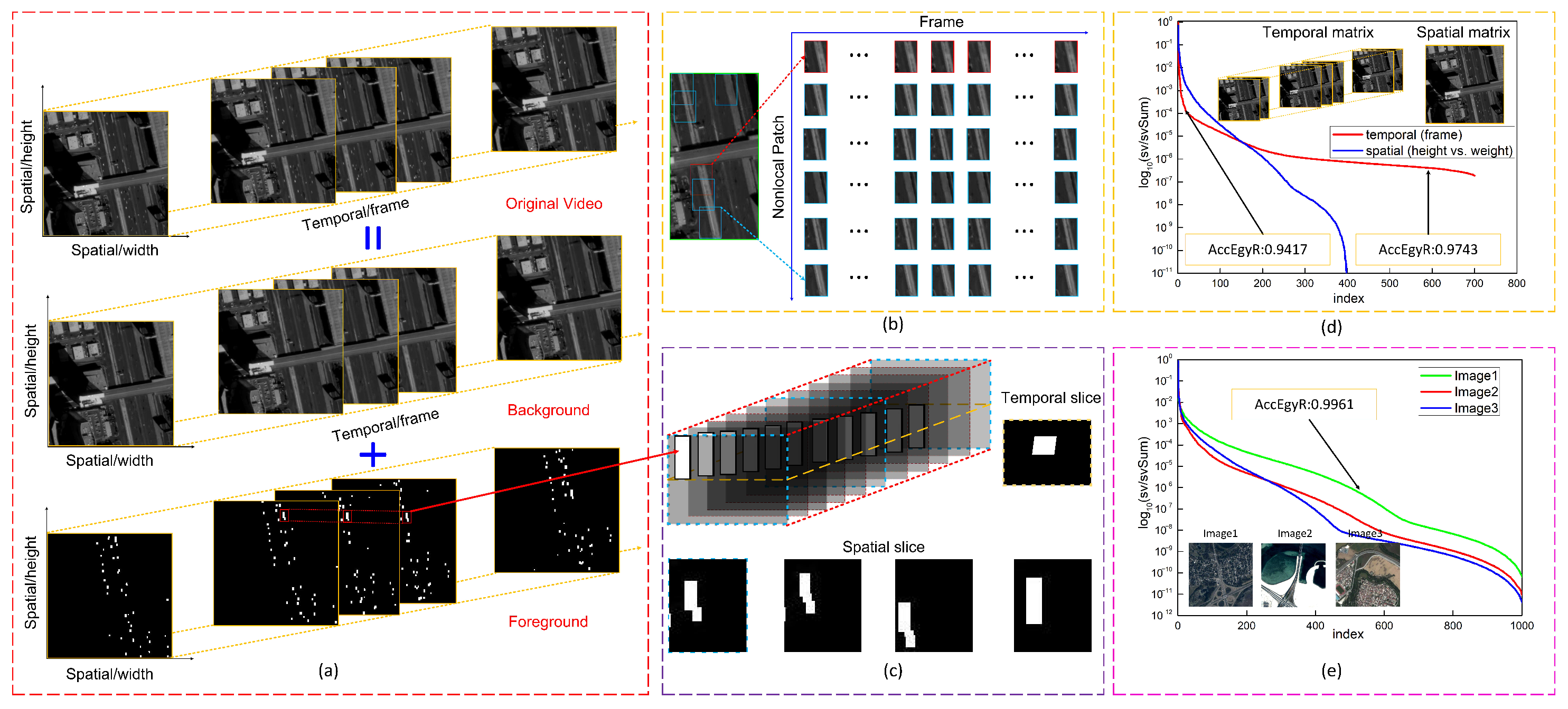
For moving object detection in satellite videos, we propose a TV regularized RPCA model to decompose a video into backgrounds and moving objects, as illustrated in Figure 2. In this section, we introduce the partial sum of singular values (PSSV) norm for background representation, aiming to reduce false alarms induced by dynamic background variations. Then, we model moving objects by the nonconvex ${\mathit{\ell }}_p$ norm to improve the recall of object detection. Next, the TV regularization is employed to suppress the changing background and local misalignment in the foreground component, and an additional error term $\mathbf{E}$ is introduced to absorb misalignment-induced background variations so that the sparse foreground $\mathbf{F}$ focuses on truly moving objects.

3.1. Preliminary Decomposition Model of Video

Given a video sequence $\mathcal{E}\in {\mathbb{R}}^{h\times w\times t}$, it is first vectorized to V∈${\mathbb{R}}^{hw\times t}$, where h, w, and t are the height, width, and the number of frames, respectively. Generally, a video sequence can be represented as

$$\mathbf{V}=\mathbf{B}+\mathbf{F},$$

(1)

where $\mathbf{B}$ is the low-rank background, and $\mathbf{F}$ is the sparse foreground that includes the moving objects.

Mathematically, the MOD problem is equivalent to solving the following problem:

$$\underset{\mathbf{B},\mathbf{F}}{min}rank\left(\mathbf{B}\right)+\lambda {\parallel \mathbf{F}\parallel }_0,s.t.\mathbf{V}=\mathbf{B}+\mathbf{F},$$

(2)

where ${∥·∥}_0$ denotes ${\mathit{\ell }}_0$ norm, and $\lambda$ is a coefficient controlling the weight of the sparse matrix F. Since Equation (2) is a nonconvex NP-hard problem, nonconvex surrogates (i.e., the nuclear norm and the ${\mathit{\ell }}_1$-norm) are used to relax Equation (2) to obtain:

$$\underset{\mathbf{B},\mathbf{F}}{min}{\parallel \mathbf{B}\parallel }_{\ast }+\lambda {\parallel \mathbf{F}\parallel }_1,s.t.\mathbf{V}=\mathbf{B}+\mathbf{F}.$$

(3)

3.2. Partial Sum of Singular Values for Background Modeling

Although the nuclear norm helps to make Equation (3) tractable, it requires multiple observations. Consequently, Equation (3) cannot be directly solved due to insufficient observations in satellite videos. Since the partial sum of minimization singular values (PSSV) [37] can preserve the large singular values while minimizing the variance in the residual rank, it is suitable to solve Equation (3). In this paper, we employ PSSV to model a low-rank background by exploiting the recurrence of image patches in a spatial–temporal neighborhood:

$$\begin{array}{c}\hfill \begin{array}{cc}\hfill \left|rank\left(\mathbf{B}\right)-N\right|& \approx \left|{\parallel \mathbf{B}\parallel }_{\ast }-{\parallel P_N\left(\mathbf{B}\right)\parallel }_{\ast }\right|\hfill \\ \hfill & =\left|\sum _{i=1}^{min(m,n)}{\delta }_i\left(\mathbf{B}\right)-\sum _{i=1}^N{\delta }_i\left(\mathbf{B}\right)\right|\hfill \\ \hfill & =\sum _{i=N+1}^{min(m,n)}{\delta }_i\left(\mathbf{B}\right)={\parallel \mathbf{B}\parallel }_{\ast ,\ast ,⩽r}={\parallel \mathbf{B}\parallel }_{p=N},\hfill \end{array}\end{array}$$

(4)

where ${\parallel \mathbf{B}\parallel }_{p=N}$ denotes the rank measure of B, ${\parallel \mathbf{B}\parallel }_{\ast ,\ast ,⩽r}$ denotes the sum of the ${(N+1)}^{th}$ to the last singular value. r represents the upper bound of the ratio between ${\delta }_N\left(\mathbf{B}\right)$ and ${\delta }_1\left(\mathbf{B}\right)$.

3.3. Nonconvex ${\mathit{\ell }}_p$ Norm for Foreground Modeling

Although ${\mathit{\ell }}_1$ norm encourages higher sparsity of F, it treats each entry (pixel) independently without considering the spatial correlation of foreground pixels. To address this problem, several works [10,11,12,14,38] adopt the ${\mathit{\ell }}_1$/${\mathit{\ell }}_{\infty }$ norm to model foreground. Unfortunately, this constraint led to the over-smoothness of the foreground. To remedy this, we propose a nonconvex constraint ${\mathit{\ell }}_p$-norm ($0<p<1$) to model the foreground. Our ${\mathit{\ell }}_p$-norm can fully exploit the spatial correlation and feature similarity while reducing the computational consumption. The ${\mathit{\ell }}_p$-norm of a foreground matrix F is defined as:

$${\parallel \mathbf{F}\parallel }_{{\mathit{\ell }}_p}={(\sum _{i=1}^m\sum _{j=1}^n\mid f_{ij}{\mid }^p)}^{{\displaystyle \frac{1}{p}}}(0<p<1),$$

(5)

By integrating Equations (4) and (5) into Equation (3), the MOD problem under a static background can be formulated as:

$$\underset{\mathbf{B},\mathbf{F}}{min}{\parallel \mathbf{B}\parallel }_{p=N}+\lambda {\parallel \mathbf{F}\parallel }_{{\mathit{\ell }}_p},s.t.\mathbf{V}=\mathbf{B}+\mathbf{F}.$$

(6)

3.4. Spatial–Temporal Continuity and Total Variation

We further impose spatial and temporal continuity prior to the foreground model to suppress the false alarms caused by local misalignment. In particular, a TV regularization is employed to enforce spatial–temporal coherence within the foreground component.

First, we calculate local variations along different axes of the video sequence $\mathcal{E}$:  

$$\begin{array}{cc}\hfill {\mathcal{E}}_h(x,y,t)& =\mathcal{E}(x+1,y,t)-\mathcal{E}(x,y,t),\hfill \\ \hfill {\mathcal{E}}_w(x,y,t)& =\mathcal{E}(x,y+1,t)-\mathcal{E}(x,y,t),\hfill \\ \hfill {\mathcal{E}}_t(x,y,t)& =\mathcal{E}(x,y,t+1)-\mathcal{E}(x,y,t),\hfill \end{array}$$

(7)

     Then, these resultant matrices are vectorized to obtain ${\mathcal{D}}_h$e = vec(${\mathcal{E}}_h$), ${\mathcal{D}}_w$e = vec(${\mathcal{E}}_w$), and ${\mathcal{D}}_t$e = vec(${\mathcal{E}}_t$). Let $\mathcal{D}$e = [${\mathcal{D}}_h{\mathit{e}}^T,{\mathcal{D}}_w{\mathit{e}}^T,{\mathcal{D}}_t{\mathit{e}}^T$] denote the concatenation of ${\mathcal{D}}_h$, ${\mathcal{D}}_w$, and ${\mathcal{D}}_t$, the anistropic total variation can be defined as:

$${\parallel \mathcal{E}\parallel }_{TV2}=\sum _i\sqrt{{\left[{\mathcal{D}}_h\mathit{e}\right]}_i^2+{\left[{\mathcal{D}}_w\mathit{e}\right]}_i^2+{\left[{\mathcal{D}}_t\mathit{e}\right]}_i^2},$$

(8)

where ${\left[{\mathcal{D}}_h\mathit{e}\right]}_i$, ${\left[{\mathcal{D}}_w\mathit{e}\right]}_i$, and ${\left[{\mathcal{D}}_t\mathit{e}\right]}_i$ represent the intensity changes along the horizontal, vertical and temporal axes, respectively. Next, the TV regularization can be used to suppress the intensity changes caused by nonstationary satellite platforms.

3.5. MOD Models

By integrating the background model (Equation (4)), the foreground model (Equation (5)), and the TV model (Equation (8)), the final MOD model can be derived:

$$\begin{array}{c}\hfill \begin{array}{cc}\hfill & \underset{\mathbf{B},\mathbf{F},\mathbf{E}}{min}{\parallel \mathbf{B}\parallel }_{p=N}+{\lambda }_1{\parallel \mathbf{F}\parallel }_{{\mathit{\ell }}_p}+{\lambda }_2{\parallel \mathbf{E}\parallel }_{TV}.\hfill \\ \hfill & s.t.\mathbf{V}=\mathbf{B}+\mathbf{F}+\mathbf{E},\hfill \end{array}\end{array}$$

(9)

where E represents content variations caused by local misalignment, which is often detected as false alarms. Unlike the sparse foreground $\mathbf{F}$, which models truly moving vehicles, $\mathbf{E}$ is used to capture dense but structured disturbances (e.g., ghosting along building edges), and is particularly important in high-resolution urban scenes with imperfect registration. By imposing a TV penalty on $\mathbf{E}$, these misalignment-induced patterns are encouraged to be spatially and temporally smooth, preventing them from leaking into $\mathbf{F}$ and thus reducing false detections. ${\lambda }_1$ and ${\lambda }_2$ are two weighting hyper-parameters. The proposed TV-RPCA model degrades to a special case, i.e., MOD in videos with static backgrounds, when ${\lambda }_2$ tends sufficiently large with fixed ${\lambda }_1$. More discussion on ${\lambda }_1$ and ${\lambda }_2$ is provided in Section 5.3.1.

4. Optimization Algorithm

In this section, we initially design an efficient ADMM-based algorithm [39,40] to address TV-RPCA as formulated in Equation (9). Subsequently, the algorithm is adapted to handle the special case described in Equation (6).

4.1. Optimization Algorithm for TV-RPCA

We optimize the TV-RPCA model through a multi-block variant of the ADMM framework, with implementation details summarized in Algorithm 1. In particular, the augmented Lagrangian corresponding to Equation (9) is expressed as:

$$\begin{array}{c}\hfill L_{\mu }(\mathbf{B},\mathbf{F},\mathbf{E},\mathbf{Y},\mu )={\parallel \mathbf{B}\parallel }_{p=N}+{\lambda }_1{\parallel \mathbf{F}\parallel }_{{\mathit{\ell }}_p}+{\lambda }_2{\parallel \mathbf{E}\parallel }_{TV}\\ \hfill +\langle \mathbf{Y},\mathbf{V}-\mathbf{B}-\mathbf{F}-\mathbf{E}\rangle +{\displaystyle \frac{\mu }{2}}{\parallel \mathbf{V}-\mathbf{B}-\mathbf{F}-\mathbf{E}\parallel }_F^2,\end{array}$$

(10)

where Y denotes the Lagrange multiplier matrix, $\mu$ is a positive penalty parameter, $\langle ·,·\rangle$ represents the matrix inner product, and ${∥·∥}_F$ is the Frobenius norm. Because joint optimization over all variables is intractable, the ADMM scheme is employed to decompose the problem into a sequence of sub-tasks:

Algorithm 1 The proposed TV-RPCA method for MOD

Require:  $\mathbf{V}\in {\mathbb{R}}^{hw\times t},{\lambda }_1>0,{\lambda }_2>0,\mu >0,\rho >0,$ and $\overline{\mu }=\mu \times {10}^7,maxIter=20.$ Ensure:  $\mathbf{B},\mathbf{F},$ and $\mathbf{E}$.   1: ${\mathbf{B}}^0={\mathbf{F}}^0={\mathbf{E}}^0={\mathbf{Y}}^0=\mathbf{0}\in {\mathbb{R}}^{hw\times t}$.   2: $\mathit{k}$ = 0   3: while not converged do   4:     Update ${\mathbf{B}}^{k+1}$ by Equation (12).   5:     Update ${\mathbf{F}}^{k+1}$ by Equation (15).   6:     Update ${\mathbf{E}}^{k+1}$ by Equation (17).   7:     Update the Lagrangian multipliers by Equation (18).   8:     Update $\mu$ by $\mu$ = min($\rho \mu ,\overline{\mu }$).   9:     Break if the termination conditions are reached. 10:    $\mathit{k}$ = $\mathit{k}$+1. 11: end while 12: return ${\mathbf{B}}^{k+1},{\mathbf{F}}^{k+1},$ and ${\mathbf{E}}^{k+1}$.

4.1.1. B Update

Updating B while keeping other variables fixed:

$$\begin{array}{c}\hfill \begin{array}{cc}\hfill {\mathbf{B}}^{k+1}& =\underset{\mathbf{B}}{\mathrm{argmin}}{L}_{\mu }(\mathbf{B},{\mathbf{F}}^k,{\mathbf{E}}^k,{\mu }_k)\hfill \\ \hfill & =\underset{\mathbf{B}}{\mathrm{argmin}}{\mu }_k^{-1}{\parallel \mathbf{B}\parallel }_{\ast ,\le r}\hfill \\ \hfill & +{\displaystyle \frac{{\mu }^k}{2}}{\parallel \mathbf{V}-{\mathbf{B}}^k-{\mathbf{F}}^k-{\mathbf{E}}^k+{\displaystyle \frac{{\mathbf{Y}}^k}{{\mu }^k}}\parallel }_F^2.\hfill \end{array}\end{array}$$

(11)

Updated B can be derived as:

$${\mathbf{B}}^{k+1}={\mathbb{P}}_{N,{\mu }_k^{-1}}(\mathbf{V}-{\mathbf{F}}^k-{\mathbf{E}}^k),$$

(12)

where ${\mathbb{P}}_{N,{\mu }_k^{-1}}$ is the Partial Singular Value Thresholding (PSVT) operator in [37]. According to [37], we can obtain

$$\begin{array}{c}\hfill \begin{array}{cc}\hfill {\mathbb{P}}_{N,\tau }\left[\mathbf{X}\right]& ={\mathbf{U}}_X({\mathbf{D}}_{X1}+{\mathbf{S}}_{\tau }\left[{\mathbf{D}}_{X2}\right]){\mathbf{V}}_X^T\hfill \\ \hfill & ={\mathbf{X}}_1+{\mathbf{U}}_{X2}({\mathbf{S}}_{\tau }\left[{\mathbf{D}}_{X2}\right]){\mathbf{V}}_{X2}^T,\hfill \end{array}\end{array}$$

(13)

where

$$\begin{array}{c}\hfill \begin{array}{cc}\hfill {\mathbf{D}}_{X1}& =diag({\delta }_1,...,{\delta }_N,0,...0),\hfill \\ \hfill {\mathbf{D}}_{X2}& =diag(0,...,0,{\delta }_{N+1},0,...0).\hfill \end{array}\end{array}$$

${\mathbf{S}}_{\tau }$ = sign(X)$·max(\left|\mathbf{X}\right|-\tau$, 0) is a soft-thresholding operator [41]. X can be decomposed using singular value decomposition (SVD) and considered to be the sum of two matrices, i.e., $\mathbf{X}={\mathbf{X}}_1+{\mathbf{X}}_2={\mathbf{U}}_{X1}{\mathbf{D}}_{X1}{\mathbf{V}}_{X1}^T+{\mathbf{U}}_{X2}{\mathbf{D}}_{X2}{\mathbf{V}}_{X2}^T$, where ${\mathbf{U}}_{X1}$ and ${\mathbf{V}}_{X1}$ are the singular vector matrices.

4.1.2. F Update

With the remaining variables in Equation (10) fixed, the foreground component F is updated by solving:  

$$\begin{array}{c}\hfill \begin{array}{cc}\hfill {\mathbf{F}}^{k+1}& =\underset{\mathbf{F}}{\mathrm{argmin}}{L}_{\mu }({\mathbf{B}}^{k+1},\mathbf{F},{\mathbf{E}}^k,{\mu }_k)\hfill \\ \hfill & =\underset{\mathbf{F}}{\mathrm{argmin}}{\lambda }_1{\mu }_k^{-1}{\parallel \mathbf{F}\parallel }_{{\mathit{\ell }}_p}\hfill \\ & +{\displaystyle \frac{{\mu }^k}{2}}{\parallel \mathbf{V}-{\mathbf{B}}^{k+1}-{\mathbf{F}}^k-{\mathbf{E}}^k+\frac{{\mathbf{Y}}^k}{{\mu }^k}\parallel }_F^2.\hfill \end{array}\end{array}$$

(14)

The optimization in Equation (14) corresponds to a standard ${\mathit{\ell }}_p$-regularized minimization problem. Consequently, the closed-form solution can be obtained via an element-wise shrinkage operator [42]:

$${\mathbf{F}}^{k+1}={\mathcal{T}}_{{\mu }_k^{-1}{\lambda }_1,p}\left(\mathbf{V}-{\mathbf{B}}^{k+1}-{\mathbf{E}}^k\right),$$

(15)

where ${\mathcal{T}}_{{\mu }^{-1}{\lambda }_1,p}(·)$ denotes the element-wise shrinkage operator.

4.1.3. E Update

During optimization, updated E can be calculated by the following steps:  

$$\begin{array}{c}\hfill \begin{array}{cc}\hfill {\mathbf{E}}^{k+1}& =\underset{\mathbf{E}}{\mathrm{argmin}}{L}_{\mu }({\mathbf{B}}^{k+1},{\mathbf{F}}^{k+1},{\mathbf{E}}^k,{\mu }_k)\hfill \\ \hfill & =\underset{\mathbf{E}}{\mathrm{argmin}}\lambda {\mu }_k^{-1}{\parallel \mathbf{E}\parallel }_{TV}\hfill \\ & +{\displaystyle \frac{{\mu }^k}{2}}{\parallel \mathbf{V}-{\mathbf{B}}^{k+1}-{\mathbf{F}}^k-{\mathbf{E}}^k+{\displaystyle \frac{{\mathbf{Y}}^k}{{\mu }^k}}\parallel }_F^2.\hfill \end{array}\end{array}$$

(16)

The solution can be obtained using the TV norm regularization strategy [43]:

$${\mathbf{E}}^{k+1}=T{V}_{{\mu }_k^{-1}{\lambda }_2}(\mathbf{V}-{\mathbf{B}}^{k+1}-{\mathbf{F}}^{k+1}),$$

(17)

where ${\mathit{TV}}_{{\mu }_k^{-1}{\lambda }_2}$ indicates the TV optimization algorithm. Updated multipliers can be obtained as:

$${\mathbf{Y}}^{k+1}={\mathbf{Y}}^k+{\mu }_k(\mathbf{V}-{\mathbf{B}}^{k+1}-{\mathbf{F}}^{k+1}-{\mathbf{E}}^{k+1}).$$

(18)

During optimization, all variables are updated iteratively until the maximum number of iterations is reached or the following criterion is satisfied:

$${\displaystyle \frac{\parallel \mathbf{V}-{\mathbf{B}}^{k+1}-{\mathbf{E}}^{k+1}-{\mathbf{F}}^{k+1}\parallel }{{\parallel \mathbf{V}\parallel }_F}}\le \tau ,$$

(19)

where $\tau$ = ${10}^{-7}$. The proposed algorithm for TV-RPCA can now be summarized in Algorithm 1.

4.2. Special Case: MOD from Static Background

In this section, we consider a special case with a static background. In this case, we set E = 0 such that Equation (9) can be modified as:

$$\begin{array}{c}\hfill \begin{array}{cc}\hfill & \underset{\mathbf{B},\mathbf{F}}{min}{\parallel \mathbf{B}\parallel }_{p=N}+\lambda {\parallel \mathbf{F}\parallel }_{{\mathit{\ell }}_p}.s.t.\mathbf{V}=\mathbf{B}+\mathbf{F}.\hfill \end{array}\end{array}$$

(20)

Then, ADMM is adopted for optimization:

4.2.1. B Update

Updating B with other terms being fixed  

$$\begin{array}{c}\hfill \begin{array}{cc}\hfill {\mathbf{B}}^{k+1}& =\underset{\mathbf{B}}{\mathrm{argmin}}{L}_{\mu }(\mathbf{B},{\mathbf{F}}^k,{\mu }_k)\hfill \\ \hfill & =\underset{\mathbf{B}}{\mathrm{argmin}}{\mu }_k^{-1}{\parallel \mathbf{B}\parallel }_{\ast ,\le r}+{\displaystyle \frac{{\mu }^k}{2}}{\parallel \mathbf{V}-{\mathbf{B}}^k-{\mathbf{F}}^k+{\displaystyle \frac{{\mathbf{Y}}^k}{{\mu }^k}}\parallel }_F^2.\hfill \end{array}\end{array}$$

(21)

Updated B can be derived as:

$${\mathbf{B}}^{k+1}={\mathbb{P}}_{N,{\mu }_k^{-1}}(\mathbf{V}-{\mathbf{F}}^k).$$

(22)

4.2.2. F Update

Updating F while fixing other variables:

$$\begin{array}{c}\hfill \begin{array}{cc}\hfill {\mathbf{F}}^{k+1}& =\underset{\mathbf{F}}{\mathrm{argmin}}{L}_{\mu }({\mathbf{B}}^{k+1},\mathbf{F},{\mu }_k)\hfill \\ \hfill & =\underset{\mathbf{F}}{\mathrm{argmin}}{\lambda }_1{\mu }_k^{-1}{\parallel \mathbf{F}\parallel }_{{\mathit{\ell }}_p}+{\displaystyle \frac{{\mu }^k}{2}}{\parallel \mathbf{V}-{\mathbf{B}}^{k+1}+{\displaystyle \frac{{\mathbf{Y}}^k}{{\mu }^k}}\parallel }_F^2.\hfill \end{array}\end{array}$$

(23)

Hence, updated F can be obtained as:

$${\mathbf{F}}^{k+1}={\mathcal{T}}_{{\mu }_k^{-1}{\lambda }_1,p}(\mathbf{V}-{\mathbf{B}}^{k+1}).$$

(24)

Similarly, updating multipliers while keeping other terms fixed:

$$\begin{array}{c}\hfill \begin{array}{cc}\hfill {\mathbf{Y}}^{k+1}& ={\mathbf{Y}}^k+{\mu }_k(\mathbf{V}-{\mathbf{B}}^{k+1}-{\mathbf{F}}^{k+1}-{\mathbf{E}}^{k+1}).\hfill \end{array}\end{array}$$

(25)

The overall algorithm is summarized in Algorithm 2.

Algorithm 2 The proposed STV-RPCA method for MOD

Require:  $\mathbf{V}\in {\mathbb{R}}^{hw\times t},\lambda >0,\mu >0,\rho >0,$ and $\overline{\mu }=\mu \times {10}^7$, $maxIter$ = 20. Ensure:  $\mathbf{B}$ and $\mathbf{F}$.   1: ${\mathbf{B}}^0={\mathbf{F}}^0={\mathbf{Y}}^0=\mathbf{0}\in {\mathbb{R}}^{hw\times t}$.   2: $\mathit{k}$ = 0   3: while not converged do   4:     Update ${\mathbf{B}}^{k+1}$ by Equation (22).   5:     Update ${\mathbf{F}}^{k+1}$ by Equation (24).   6:     Update the Lagrangian multipliers by Equation (25).   7:     Update $\mu$ by $\mu$ = min($\rho \mu ,\overline{\mu }$).   8:     Break if the termination conditions are reached.   9:     $\mathit{k}$ = $\mathit{k}$+1. 10: end while 11: return ${\mathbf{B}}^{k+1}$ and ${\mathbf{F}}^{k+1}$.

5. Results

In this section, experiments are performed on the VISO and SkySat datasets to validate the advantages of the proposed TV-RPCA model compared with representative state-of-the-art MOD methods. The composition of the VISO and SkySat datasets is shown in

Table 1. Information of the evaluation datasets.

Dataset	Name	Frame Size × Frames	Frame Rate	Time Cost (s)
VISO	Video 001–006	1024 × 1024 × 325	10 Hz	4564
	Video 007	1024 × 1024 × 300	10 Hz	4028
SkySat	Video 008	400 × 400 × 700	30 Hz	486
	Video 009	600 × 600 × 700	30 Hz	892

. All implementations are carried out in MATLAB 2021 on a workstation equipped with an AMD Ryzen-3990X CPU. For other methods, we finetune their parameters to achieve the best F1 scores for evaluation.

5.1. Metrics

In our experiments, recall, precision, F1 scores are used as metrics:

$$\mathrm{Recall}={\displaystyle \frac{TP}{TP+FN}},$$

(26)

$$\mathrm{Precision}={\displaystyle \frac{TP}{TP+FP}},$$

(27)

$$F1={\displaystyle \frac{2\times \mathrm{Recall}\times \mathrm{Precision}}{\mathrm{Recall}+\mathrm{Precision}}},$$

(28)

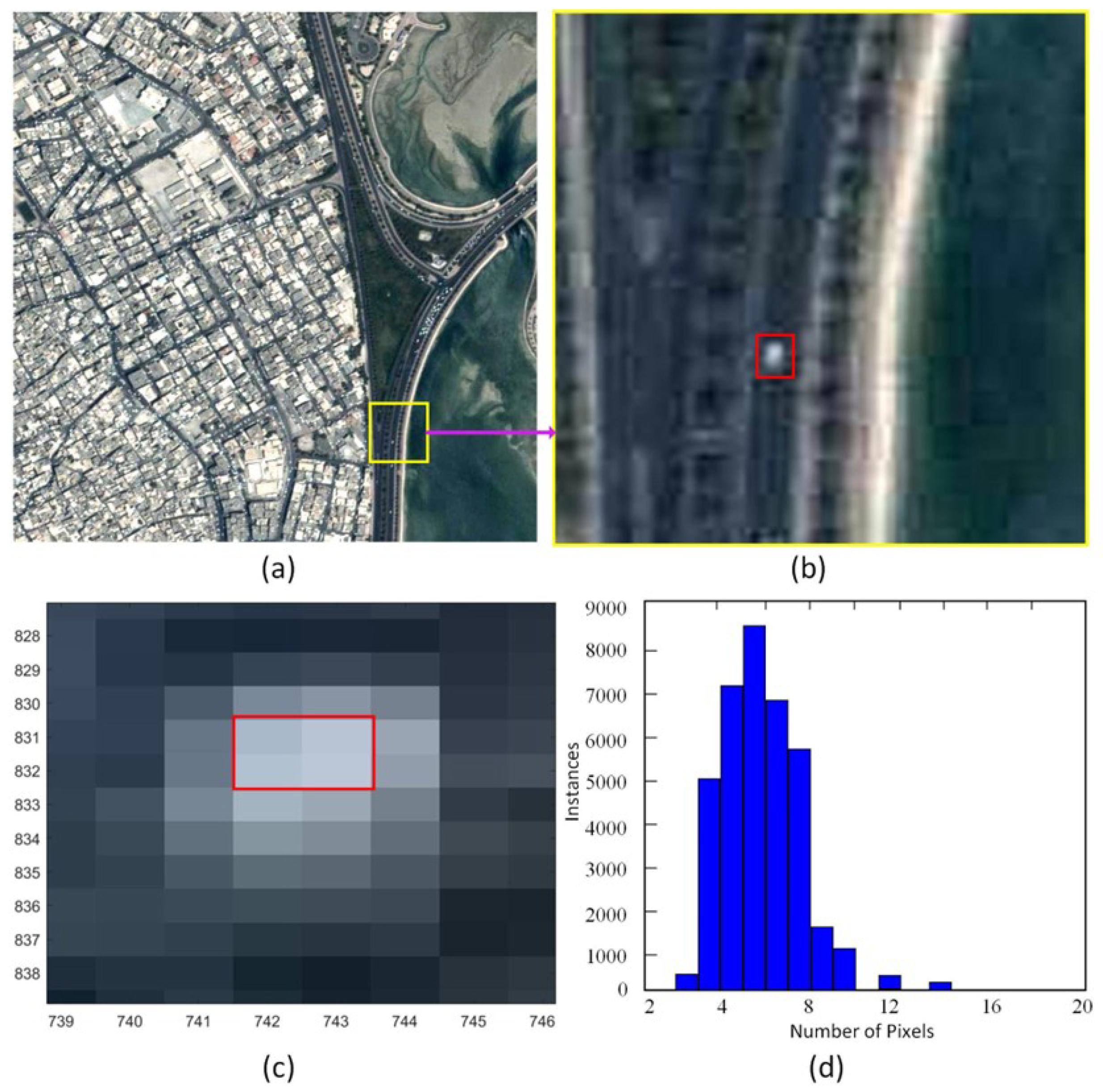
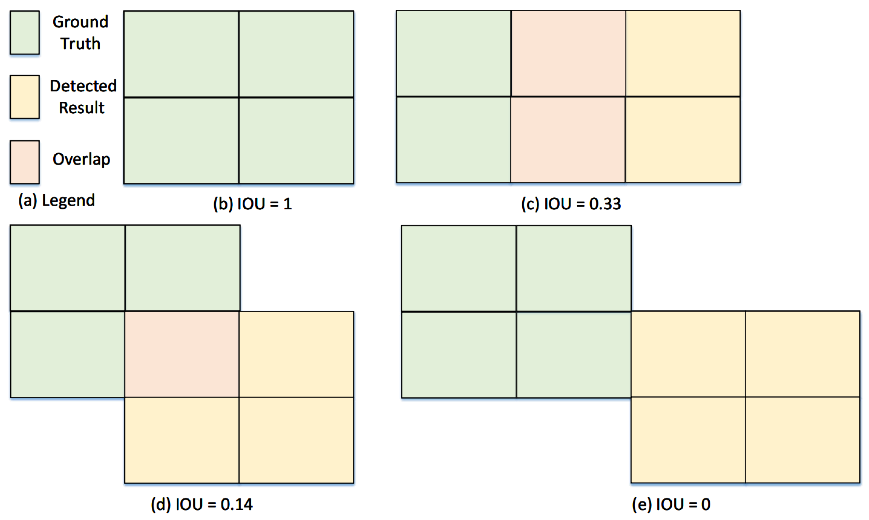
here, $\mathit{FP}$, $\mathit{TP}$, and $\mathit{FN}$ denote the number of false positives, true positives, and false negatives, respectively. The F1 metric provides a balanced measure by combining recall and precision, offering a comprehensive evaluation criterion [44]. Although IoU has been widely used as an evaluation metric for generic object detection in the literature [45], it is not particularly suitable for our case, due to the low spatial resolution of satellite remote sensing videos and extremely small objects. As shown in Figure 3d, the majority of the vehicles in our dataset only occupy about 2 20 pixels. In this case, the conventional IoU metric is quite sensitive to the predictions. Taking Figure 4 as an example, the object size is around 4 pixels, and tiny shifts of the predicted bounding box (i.e., 1 or 2 pixels) will cause a large fluctuation of the IoU score. Therefore, we instead consider a predicted detection as a true positive if the predicted bounding box overlaps with the ground truth bounding box. Larger values of recall, precision, and F1 indicate superior detection performance.

5.2. Datasets

5.2.1. The VISO Dataset

The VISO dataset [13] was collected by the Jilin-1 satellite operated by Changguang Satellite Technology Co., Ltd., Changchun, China (http://www.jl1.cn/index.aspx/, accessed on 21 December 2025). It comprises 47 high-resolution satellite video sequences (1.0 m GSD, 10 fps) captured over diverse orbital locations. Following prior work, we employ the official test split, which includes seven sequences (Video 001–007) spanning a wide range of scene conditions, from static backgrounds to highly dynamic environments. VISO is characterized by dense traffic scenes, containing up to 200 vehicles per frame (typically over 100), most of which are extremely small targets. Approximately 90% of the objects occupy fewer than 50 pixels (commonly 4 × 4 to 20 × 20 pixels). Each object is annotated with an axis-aligned bounding box and a unique identity for multi-frame tracking. IDs are initially assigned in the first frame and then cross-verified throughout the sequence to ensure temporal consistency. All annotations were manually checked to guarantee quality across the dataset.

5.2.2. The SkySat Dataset

The SkySat dataset was captured over Las Vegas, USA, by SkySat-1 on 25 March 2014, with a ground sampling distance of 1.0 m and a frame rate of 30 fps. We follow the standard evaluation protocol and use two grayscale sequences (Video 008 and Video 009, 700 frames each), with manually annotated vehicle bounding boxes (https://github.com/zhangjunpeng9354/satellite_video_mod_groundtruth, accessed on 21 December 2025). SkySat features moderate traffic density (50–100 vehicles per frame) and small object sizes (mostly < 50 pixels). Video 008 contains complex backgrounds and noticeable local misalignment, whereas Video 009 presents a relatively stable scene. Annotations were generated semi-automatically and then manually refined to ensure accuracy and temporal consistency.

5.3. Parameter Analysis

5.3.1. Parameter Settings

As suggested in RPCA [46,47,48,49]. $\lambda$ is set to $1/\sqrt{hw}$, where $\mathit{h}$ and $\mathit{w}$ are the width and height of each video. For video sequences with static backgrounds, we empirically set ${\lambda }_1=1.2/\sqrt{hw}$. For video sequences with complex and dynamic backgrounds, we empirically set ${\lambda }_1=1.2/\sqrt{hw}$ and ${\lambda }_2=0.1/\sqrt{hw}$. In addition, we set $\mu =0.05$, and $\rho =1.5$ throughout the experiments.

5.3.2. Effect of p in ${\mathit{\ell }}_p$ Norm

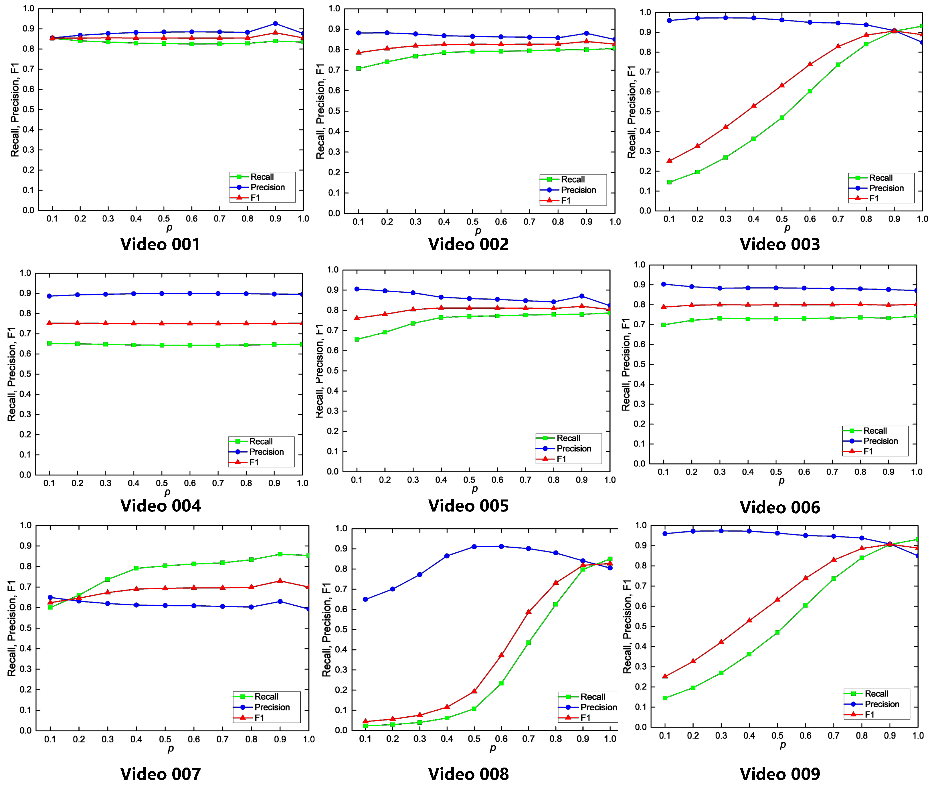
Our TV-RPCA model adopts ${\mathit{\ell }}_p$ norm for optimization and p ($0\le p\le 1$) is a critical factor. Figure 5 illustrates the value of recall, precision, and F1 scores with p varying from 0.1 to 1. As we can see, p = 0.9 and p = 1 produce better performance. Due to the dynamic backgrounds, the performance of p = 1 is slightly worse than that of p = 0.9, which validates the effectiveness of ${\mathit{\ell }}_p$ norm. Therefore, p = 0.9 is used as the default setting in the experiments.

5.4. Performance Evaluation

The proposed method is further compared with 13 state-of-the-art counterpart, including DECOLOR [50], Godec [51], ClusterNet [9], DTTP [7], D&T [8], E-LSD [10], B-MCMD [14], MMB [13], WSNM [23], DSF-Net [34], DE-TFD [18], HiEUM [36] and UMOD [52]. Among these approaches, ClusterNet [9], DSF-Net [34], DE-TFD [18], HiEUM [36], and UMOD [52] are deep learning-based methods, D&T [8] and MMB [13] are foreground detection-based method. The remaining methods are background modeling-based methods.

5.4.1. The VISO Dataset

The quantitative comparison of different methods is summarized in

Table 2. Recall (Re), Precision (Pr), and F1 values achieved by different methods on seven satellite videos of the VISO dataset. Best and second-best results are highlighted and underlined, respectively.

Method	Video 001			Video 002			Video 003			Video 004
	Re ↑	Pr ↑	F1 ↑	Re ↑	Pr ↑	F1 ↑	Re ↑	Pr ↑	F1 ↑	Re ↑	Pr ↑	F1 ↑
DSFNet [34]	91%	92%	92%	88%	85%	86%	95%	81%	88%	82%	91%	86%
ClusterNet [9]	74%	63%	68%	61%	75%	67%	81%	65%	72%	47%	68%	56%
UMOD [52]	83%	90%	86%	76%	88%	81%	90%	88%	89%	65%	83%	73%
DE-TFD [18]	88%	90%	89%	91%	86%	88%	94%	85%	89%	90%	86%	88%
HiEUM [36]	86%	97%	91%	82%	97%	89%	78%	97%	86%	92%	96%	94%
D&T [8]	70%	90%	79%	67%	82%	74%	82%	81%	82%	72%	79%	76%
MMB [13]	80%	94%	86%	71%	88%	79%	85%	90%	88%	74%	81%	78%
Godec [51]	84%	77%	80%	78%	78%	78%	72%	77%	75%	63%	78%	70%
DECOLOR [50]	36%	99%	53%	80%	81%	81%	90%	78%	83%	43%	99%	60%
DTTP [7]	74%	48%	58%	66%	80%	72%	73%	82%	77%	55%	58%	56%
E-LSD [10]	71%	76%	73%	64%	39%	48%	75%	87%	81%	57%	87%	69%
B-MCMD [14]	75%	91%	82%	71%	80%	75%	79%	74%	76%	67%	68%	68%
WSNM [23]	84%	70%	77%	79%	85%	82%	91%	87%	89%	65%	87%	74%
TV-RPCA (Ours)	80%	92%	85%	80%	88%	84%	91%	88%	90%	65%	85%	74%
Method	Video 005			Video 006			Video 007			Average
	Re ↑	Pr ↑	F1 ↑	Re ↑	Pr ↑	F1 ↑	Re ↑	Pr ↑	F1 ↑	Re ↑	Pr ↑	F1 ↑
DSFNet [34]	95%	67%	79%	81%	86%	83%	83%	87%	85%	88%	84%	86%
ClusterNet [9]	74%	79%	76%	73%	68%	71%	83%	64%	72%	71%	69%	69%
UMOD [52]	72%	89%	80%	73%	86%	79%	83%	74%	82%	77%	85%	81%
DE-TFD [18]	88%	80%	84%	83%	87%	84%	84%	92%	88%	88%	87%	87%
HiEUM [36]	82%	98%	89%	84%	96%	90%	85%	93%	88%	84%	96%	74%
D&T [8]	61%	77%	68%	62%	72%	67%	84%	39%	53%	71%	75%	71%
MMB [13]	68%	83%	75%	66%	84%	74%	86%	66%	74%	76%	84%	79%
Godec [51]	77%	71%	74%	67%	65%	66%	27%	38%	32%	67%	69%	68%
DECOLOR [50]	79%	75%	77%	78%	64%	71%	33%	70%	45%	63%	81%	67%
DTTP [7]	53%	68%	60%	53%	68%	60%	23%	47%	30%	57%	64%	59%
E-LSD [10]	61%	82%	70%	53%	75%	62%	59%	58%	58%	63%	72%	66%
B-MCMD [14]	53%	76%	63%	63%	65%	64%	77%	41%	53%	69%	71%	69%
WSNM [23]	76%	85%	80%	72%	83%	77%	73%	77%	75%	77%	82%	79%
TV-RPCA (Ours)	78%	87%	82%	72%	85%	78%	86%	63%	73%	79%	84%	81%

. It can be observed that TV-RPCA achieves competitive moving object detection (MOD) performance in terms of both precision and recall. Notably, our method attains the highest precision of 84% while maintaining a recall performance comparable to other state-of-the-art approaches. As a result, TV-RPCA achieves an F1 score of 81%, yielding an overall performance improvement of approximately 10% compared with the foreground-based method D&T [8]. This performance gap arises because D&T is unable to model dynamic backgrounds and is highly sensitive to background variations, which limits its effectiveness in complex satellite video scenes.

Compared with the strongest background modeling-based method, namely WSNM, TV-RPCA exhibits consistent performance gains in both MOD accuracy and background reconstruction quality. This advantage stems from the incorporation of spatio–temporal TV regularization, which facilitates a more accurate separation of background and foreground components. In comparison with the best deep learning-based method, DSFNet, TV-RPCA achieves comparable recall performance while delivering higher precision, demonstrating its strong capability in suppressing false alarms without sacrificing detection completeness. Overall, these results indicate that TV-RPCA provides a more balanced trade-off between precision and recall than existing methods.

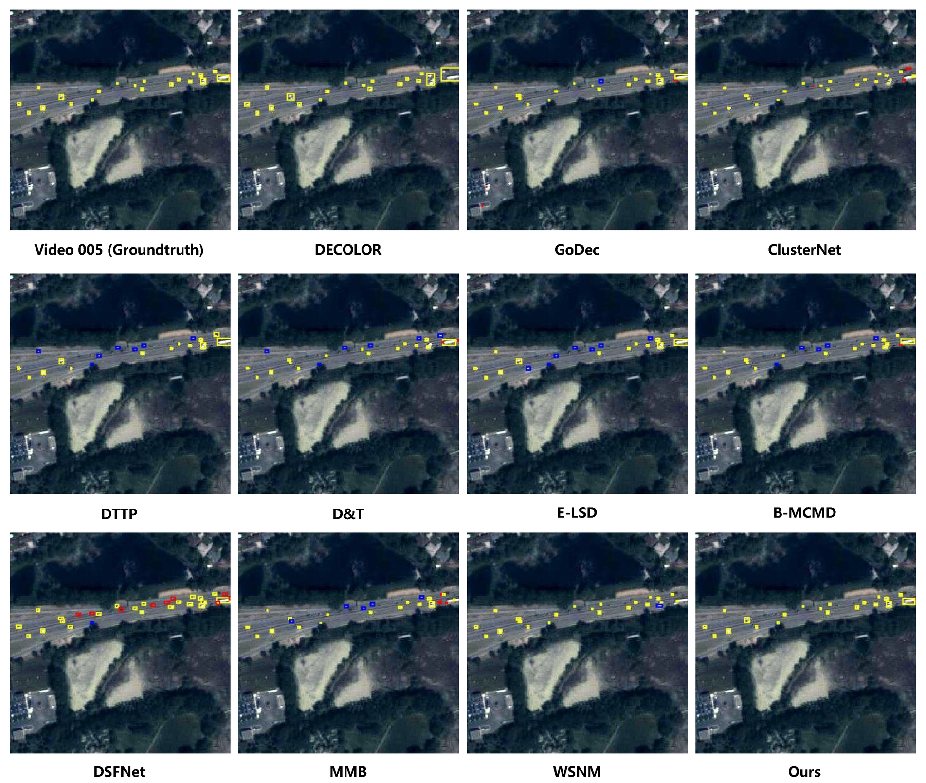
The superior quantitative performance is further corroborated by the qualitative results shown in Figure 6. As illustrated, most previous methods generate noticeable false alarms caused by local misalignments and intensity variations in satellite videos. In contrast, the proposed method produces cleaner background–foreground separation results with significantly fewer false detections. This robustness can be mainly attributed to the partial-sum low-rank background modeling together with the joint ${\mathit{\ell }}_p$ norm and spatio–temporal total variation regularization, which effectively suppresses background clutter while preserving the structural and temporal continuity of moving targets in complex scenes. Consequently, TV-RPCA achieves the best precision performance among all compared approaches.

5.4.2. The SkySat Dataset

To further validate the effectiveness of the proposed method, additional experiments are conducted on the SkySat dataset. As the SkySat dataset contains only two video sequences, DSFNet and ClusterNet models trained on the VISO dataset are directly adopted for evaluation. The experimental results demonstrate that TV-RPCA consistently outperforms state-of-the-art methods on this dataset.

Quantitative comparisons are reported in

Table 3. Recall (Re), Precision (Pr), and F1 values achieved by different methods on two satellite videos of the SkySat dataset. Best and second-best results are highlighted and underlined.

Method	Video 008			Video 009			Average			Time Cost(s)
	Re ↑	Pr ↑	F1 ↑	Re ↑	Pr ↑	F1 ↑	Re ↑	Pr ↑	F1 ↑
DSFNet [34]	88%	65%	75%	90%	78%	84%	89%	71%	79%	0.29
ClusterNet [9]	77%	46%	57%	79%	58%	66%	78%	52%	62%	0.40
UMOD [52]	51%	80%	62%	53%	82%	64%	52%	81%	63%	0.48
HiEUM [36]	95%	78%	85%	92%	82%	87%	93%	80%	87%	0.01
D&T [8]	78%	59%	67%	75%	85%	80%	76%	72%	73%	0.12
MMB [13]	68%	82%	75%	63%	84%	72%	66%	83%	73%	0.38
Godec [51]	95%	36%	52%	90%	81%	85%	93%	59%	69%	0.49
DECOLOR [50]	77%	59%	67%	79%	81%	80%	78%	70%	73%	0.72
DTTP [7]	80%	67%	73%	74%	94%	83%	77%	80%	78%	0.60
E-LSD [10]	85%	79%	82%	80%	94%	86%	82%	86%	84%	31.20
B-MCD [14]	82%	84%	85%	80%	95%	87%	81%	90%	86%	92.41
WSNM [23]	94%	76%	84%	95%	80%	87%	94%	78%	86%	0.33
TV-RPCA (Ours)	92%	88%	90%	92%	92%	92%	92%	90%	91%	0.19

. The proposed method achieves the highest F1 score of 91%, representing an improvement of 18% over the foreground-based method D&T. Compared with background modeling-based approaches, TV-RPCA exhibits notably better detection performance, which can be attributed to the incorporation of TV regularization that facilitates more accurate background–foreground separation. For Video 009, which contains relatively simple background structures, most competing methods achieve favorable results. However, even under this setting, TV-RPCA maintains superior overall performance. Compared with the deep learning-based method HiEUM, our approach improves precision by 10% and increases the F1 score by 4%. This performance gap mainly arises from the domain discrepancy between the VISO and SkySat datasets, which limits the generalization capability of HiEUM.

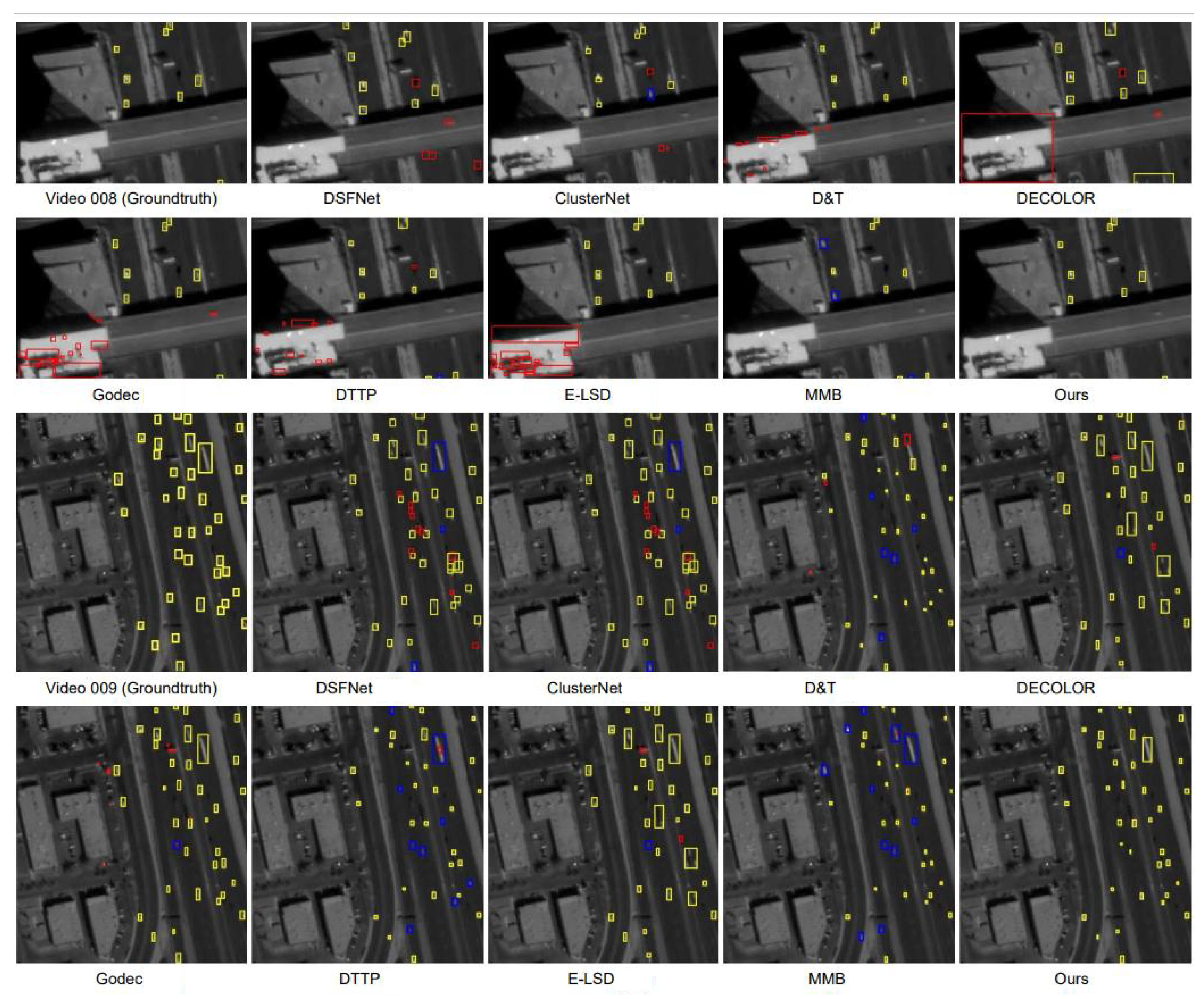
Qualitative results are presented in Figure 7. Due to local misalignment between adjacent frames, several existing methods generate noticeable false alarms in Video 008. In contrast, the proposed TV-RPCA, benefiting from spatio–temporal TV regularization, effectively suppresses such false detections and produces cleaner foreground extraction results. Moreover, with the incorporation of PPSV regularization for background modeling, the proposed method achieves more accurate background reconstruction and attains high recall performance on Video 009.

The efficiency comparison between the proposed method and other approaches is summarized in the last column of Table 3, where the average processing time is measured on input images of size $1024\times 1024$. Compared with other background modeling-based methods, TV-RPCA achieves at least a threefold acceleration. This efficiency gain is primarily due to the fact that regularization constraints are imposed on the gradient maps rather than directly on the original video sequences, significantly reducing computational complexity.

Overall, the experimental results on the SkySat dataset further demonstrate the robustness of the proposed method across different scene conditions. This robustness mainly stems from the spatio–temporal TV constraint, which preserves motion consistency across consecutive frames while effectively suppressing background-induced false responses.

5.5. Ablation Study

5.5.1. Effectiveness of Background Reconstruction

To assess the contribution of the background reconstruction module, we substitute it with several alternative strategies, including the spatial mean filter, spatial median filter, temporal mean filter, and temporal median filter. The quantitative evaluation is summarized in

Table 4. Performance of different background reconstruction methods. Average recall (Avg Re), average precision (Avg Pr), and average F1 score (Avg F1) are listed in the table for performance comparison. Best and second-best results are highlighted and underlined.

Methods	Avg Re	Avg Pr	Avg F1
spatial mean filter	32%	19%	27%
Spatial median filter	46%	19%	25%
Temporal mean filter	74%	86%	79%
Temporal median filter	73%	88%	79%
TV-RPCA (Ours)	79%	84%	81%

. It can be observed that the proposed method yields the highest F1 score, surpassing the second-best reconstruction strategy by a margin of 2 in terms of F1.

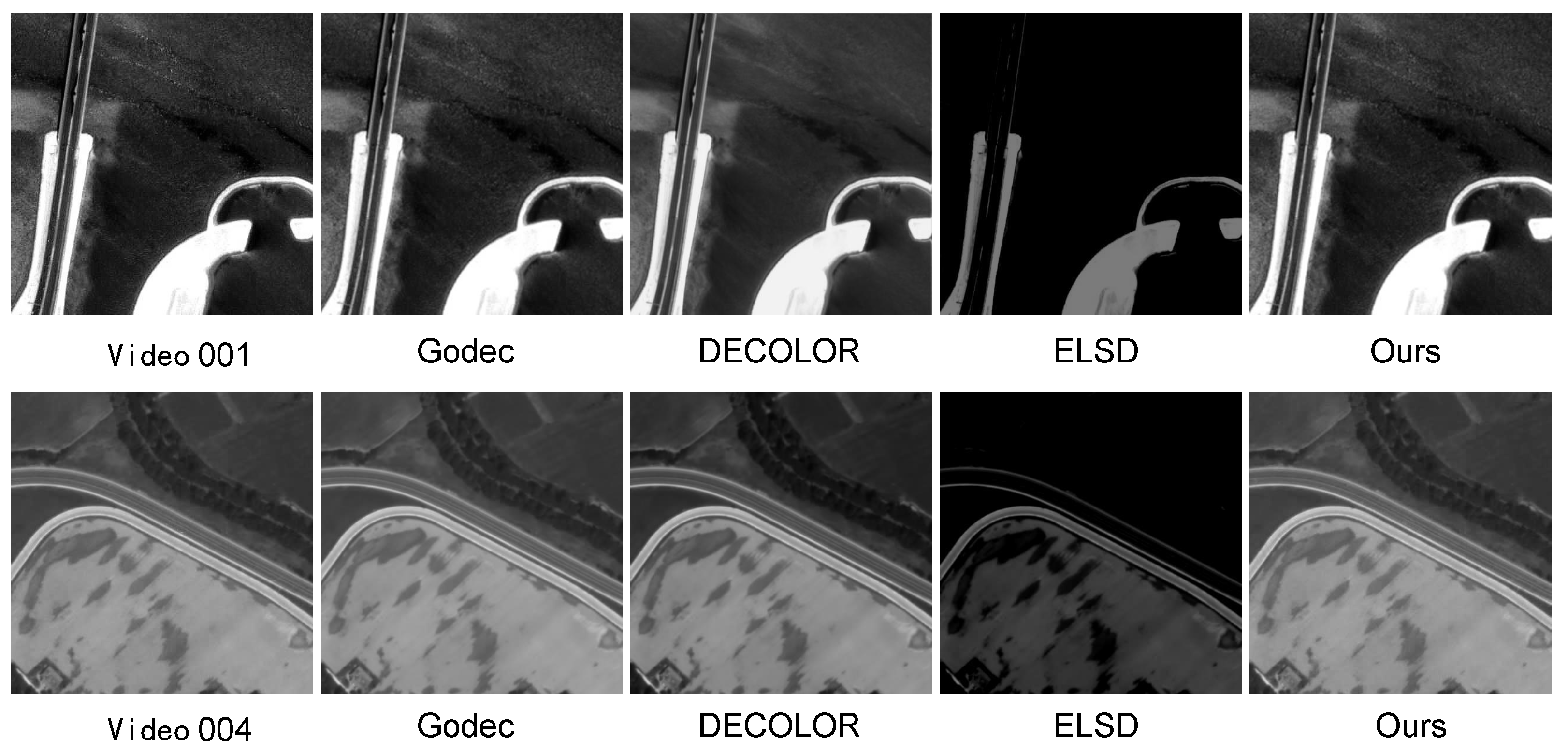
The backgrounds reconstructed by different approaches are illustrated in Figure 8. It can be observed that the proposed method is more effective in recovering clean backgrounds, thereby facilitating improved detection results. In contrast, alternative reconstruction strategies leave noticeable object residuals within target regions, leading to degraded detection accuracy.

The capability of different approaches in reconstructing backgrounds is rigorously tested by generating moving objects on clean backgrounds and then applying multiple reconstruction strategies. Following [53], PSNR and SSIM values between the reconstructed backgrounds and the ground-truth ones are adopted as quantitative metrics. We further compare our method with three representative RPCA-based approaches, namely DECOLOR [50], E-LSD [10], and Godec [51]. The corresponding quantitative results are summarized in

Table 5. Performance of different methods on the synthetic data. Average recall (Avg Re), average precision (Avg Pr), average F1 score (Avg F1), and PSNR are listed in the table for performance comparison. Best and second-best results are highlighted and underlined.

Methods	Avg Re	Avg Pr	Avg F1	PSNR	SSIM
Godec [51]	67%	69%	68%	32.88	0.96
DECOLOR [50]	63%	81%	67%	24.32	0.83
E-LSD [10]	63%	72%	66%	21.99	0.85
UMOD [52]	77%	85.3%	81%	29.87	-
TV-RPCA (Ours)	79%	84%	81%	35.44	0.96

. It is evident that our method achieves the highest PSNR and SSIM scores, confirming its superiority in reconstructing accurate backgrounds and consequently enhancing detection performance.

5.5.2. Effectiveness of Key Block

In this part, we perform ablation studies to examine the contributions of three essential components in our framework, namely low-rank background regularization, sparse foreground regularization, and total variation (TV) regularization. The specific results are shown in

Table 6. Recall (Re), Precision (Pr), and F1 scores achieved by different methods on the VISO dataset and the SkySat dataset. Best and second-best results are highlighted and underlined.

Model	Configuration			Dataset
	Background	Foreground	TV	VISO			SkySat
	Regularization	Regularization	Regularization	Re	Pr	F1	Re	Pr	F1
baseline	Nuclear norm	${\mathit{\ell }}_1$ norm	-	63%	81%	67%	78%	70%	73%
(1)	PSSV norm	${\mathit{\ell }}_1$ norm	-	78%	68%	71%	81%	85%	83%
(2)	Nuclear norm	${\mathit{\ell }}_p$ norm	-	80%	66%	72%	94%	63%	75%
(3)	PSSV norm	${\mathit{\ell }}_p$ norm	-	80%	70%	74%	88%	80%	83%
(4)	PSSV norm	${\mathit{\ell }}_1$ norm	✓	79%	68%	72%	84%	83%	83%
(5)	Nuclear norm	${\mathit{\ell }}_p$ norm	✓	76%	72%	73%	84%	84%	84%
TV-RPCA (Ours)	PSSV norm	${\mathit{\ell }}_p$ norm	✓	79%	84%	81%	82%	86%	84%

. We first develop a baseline model using the nuclear norm to model the background and the ${\mathit{\ell }}_p$ regularization to encode the foreground. Then, we introduce Model (1), Model (2), and Model (3) by adopting the low-rank background regularization and ${\mathit{\ell }}_p$ foreground regularization. Compared to the baseline model, low-rank background regularization facilitates Model (1) to achieve improved performance, with F1 scores of 71% and 83% on the VISO and SkySat datasets, respectively. Moreover, the ${\mathit{\ell }}_p$ foreground regularization also helps Model (2) to achieve a higher recall score of 80% and 94% on VISO and SkySat, respectively. By combining both regularizations, Model (3) achieves superior MOD performance in terms of both recall and F1, which demonstrates the effectiveness of these regularizations. To validate the TV regularization, we introduce three variants by adding TV regularization to Models (1)–(3). It can be observed that the TV regularization helps to suppress the false alarms to achieve better MOD performance.

5.6. Computational Complexity and Running Time

In this section, we provide an analysis of the computational complexity of TV-RPCA. For a video sequence containing n frames, each outer iteration consists of four update steps corresponding to B, F, E, and the Lagrange multipliers. The complexity of updating B is $O(m^{2}t+m{t}^2+t^3)$, where m denotes the product of image height and width. The updates for F and the multipliers require $O\left(mt\right)$. Moreover, the update of E incurs a cost of $O\left(k\right(mtlog\left(mt\right)\left)\right)$, where k is the number of inner iterations, fixed as 20 in our experiments. Overall, the computational complexity of a single outer iteration can be summarized as:

$$\begin{array}{cc}\hfill & O(m^{2}t+m{t}^2+t^3+2mt+10\left(mt\log \left(mt\right)\right)\hfill \\ \hfill & =O(m^{2}t+m{t}^2+t^3).\hfill \end{array}$$

(29)

In our experiments, E-LSD took 13,030 s to process a video with 325 frames of 1024 × 1024. In contrast, our TV-RPCA achieves much higher efficiency with a $3.6\times$ speedup.

6. Discussion

The results presented in Section 5 reveal several key characteristics of the proposed TV-RPCA framework for satellite video MOD. Overall, the method achieves strong precision while maintaining balanced recall across heterogeneous satellite scenes, including those affected by platform-induced misalignment and dynamic backgrounds. This performance stability suggests that explicit decomposition remains a competitive paradigm, particularly when compared with supervised learning approaches that exhibit sensitivity to domain shift.

The empirical evidence indicates that the integration of partial-sum low-rank background modeling with ${\mathit{\ell }}_p$-norm sparsity and spatio–temporal total variation priors plays a central role in enabling robust detection. These structured priors jointly enforce temporal and spatial consistency during decomposition, suppressing background leakage and enhancing the continuity of detected targets under realistic imaging perturbations. The ablation experiments further demonstrate that each regularization contributes complementary benefits, confirming the importance of combining low-rank and sparsity constraints with temporal smoothness.

Despite these strengths, two notable limitations are observed in the analysis. The fixed regularization coefficients do not adapt to heterogeneous motion patterns or rapid scene dynamics, leading to performance degradation in highly cluttered environments. Moreover, the iterative optimization introduces non-negligible computational overhead for long-duration sequences or ultra-high-resolution frames, suggesting that further acceleration is required for real-time deployment.

Taken together, the findings imply that analytically constrained decomposition-based MOD methods retain robustness advantages in scenarios where annotation is limited or environments diverge from training domains. At the same time, the identified limitations motivate future research into adaptive regularization, GPU-aware optimization, and hybrid formulations that combine decomposition priors with lightweight learned representations.

7. Conclusions

In this paper, we propose a robust PCA-based framework for moving-vehicle detection in satellite videos. The background is modeled using the partial sum of singular values (PSSV), while the foreground is characterized by the joint ${\mathit{\ell }}_p$ norm and total variation (TV) regularization to promote sparsity and spatio–temporal continuity. Extensive experiments on the SkySat and VISO datasets demonstrate that the proposed method achieves strong detection accuracy and favorable computational efficiency under complex and dynamic background conditions. However, the current foreground modeling strategy relies on fixed regularization forms, which may limit its flexibility when dealing with highly heterogeneous motion patterns or complex foreground distributions in more diverse satellite video scenarios.

8. Future Work

To address the aforementioned limitation in modeling highly diverse foreground dynamics, future work will focus on enhancing the flexibility and expressiveness of the proposed framework. One potential direction is to incorporate mixture-of-Gaussians representations to better capture heterogeneous motion patterns and complex foreground distributions. Furthermore, semi-supervised learning paradigms based on graph signal processing and graph neural networks could be explored to adaptively model spatio–temporal relationships in satellite videos. Recent studies [54,55,56] have shown that graph-based methods are effective in handling non-Euclidean dependencies, motivating future investigations into adaptive graph constructions and temporal modeling strategies that improve robustness to occlusions and intermittent target appearances. These extensions are expected to alleviate the above-mentioned modeling constraints while preserving the computational efficiency of the proposed method.

References

1. Yi, S.; Liu, X.; Li, J.; Chen, L. Uavformer: A composite transformer network for urban scene segmentation of uav images. Pattern Recognit. 2023, 133, 109019. [Google Scholar] [CrossRef]
2. Pang, D.; Shan, T.; Ma, Y.; Ma, P.; Hu, T.; Tao, R. LRTA-SP: Low rank tensor approximation with saliency prior for small target detection in infrared videos. IEEE Trans. Aerosp. Electron. Syst. 2024, 61, 2644–2658. [Google Scholar] [CrossRef]
3. Cong, Y.; Fan, B.; Hou, D.; Fan, H.; Liu, K.; Luo, J. Novel event analysis for human-machine collaborative underwater exploration. Pattern Recognit. 2019, 96, 106967. [Google Scholar] [CrossRef]
4. Wu, J.; Ni, R.; Chen, Z.; Huang, F.; Chen, L. FEFN: Feature Enhancement Feedforward Network for Lightweight Object Detection in Remote Sensing Images. Remote Sens. 2024, 16, 2398. [Google Scholar] [CrossRef]
5. Kumar, K.N.; Roy, D.; Suman, T.A.; Vishnu, C.; Mohan, C.K. TSANet: Forecasting traffic congestion patterns from aerial videos using graphs and transformers. Pattern Recognit. 2024, 155, 110721. [Google Scholar] [CrossRef]
6. Wu, J.; Luo, C.; Qiu, Z.; Chen, L.; Ni, R.; Li, Y.; Huang, F.; Wu, J. DFINet: Dynamic feedback iterative network for infrared small target detection. Pattern Recognit. 2025, 169, 111958. [Google Scholar] [CrossRef]
7. Ahmadi, S.A.; Ghorbanian, A.; Mohammadzadeh, A. Moving vehicle detection, tracking and traffic parameter estimation from a satellite video: A perspective on a smarter city. Int. J. Remote Sens. 2019, 40, 8379–8394. [Google Scholar] [CrossRef]
8. Ao, W.; Fu, Y.; Hou, X.; Xu, F. Needles in a haystack: Tracking city-scale moving vehicles from continuously moving satellite. IEEE Trans. Image Process. 2019, 29, 1944–1957. [Google Scholar] [CrossRef]
9. LaLonde, R.; Zhang, D.; Shah, M. Clusternet: Detecting small objects in large scenes by exploiting spatio-temporal information. In Proceedings of the IEEE Conference on Computer Vision and Pattern Recognition, Salt Lake City, UT, USA, 18–23 June 2018; pp. 4003–4012. [Google Scholar]
10. Zhang, J.; Jia, X.; Hu, J. Error bounded foreground and background modeling for moving object detection in satellite videos. IEEE Trans. Geosci. Remote Sens. 2019, 58, 2659–2669. [Google Scholar] [CrossRef]
11. Zhang, J.; Jia, X.; Hu, J.; Chanussot, J. Online structured sparsity-based moving-object detection from satellite videos. IEEE Trans. Geosci. Remote Sens. 2020, 58, 6420–6433. [Google Scholar] [CrossRef]
12. Zhang, J.; Jia, X. Improved low rank plus structured sparsity and unstructured sparsity decomposition for moving object detection in satellite videos. In Proceedings of the IGARSS 2019 IEEE International Geoscience and Remote Sensing Symposium, Yokohama, Japan, 28 July–2 August 2019; pp. 5421–5424. [Google Scholar]
13. Yin, Q.; Hu, Q.; Liu, H.; Zhang, F.; Wang, Y.; Lin, Z.; An, W.; Guo, Y. Detecting and Tracking Small and Dense Moving Objects in Satellite Videos: A Benchmark. IEEE Trans. Geosci. Remote Sens. 2021, 60, 5612518. [Google Scholar] [CrossRef]
14. Zhang, J.; Jia, X.; Hu, J.; Tan, K. Moving vehicle detection for remote sensing video surveillance with nonstationary satellite platform. IEEE Trans. Pattern Anal. Mach. Intell. 2021, 44, 5185–5198. [Google Scholar] [CrossRef]
15. Cao, Y.; Wang, G.; Yan, D.; Zhao, Z. Two algorithms for the detection and tracking of moving vehicle targets in aerial infrared image sequences. Remote Sens. 2015, 8, 28. [Google Scholar] [CrossRef]
16. Saleemi, I.; Shah, M. Multiframe many–many point correspondence for vehicle tracking in high density wide area aerial videos. Int. J. Comput. Vis. 2013, 104, 198–219. [Google Scholar] [CrossRef]
17. Keck, M.; Galup, L.; Stauffer, C. Real-time tracking of low-resolution vehicles for wide-area persistent surveillance. In Proceedings of the IEEE/CVF Workshop on Applications of Computer Vision (WACV), Clearwater Beach, FL, USA, 15–17 January 2013; pp. 441–448. [Google Scholar]
18. Pi, Z.; Jiao, L.; Liu, F.; Liu, X.; Li, L.; Hou, B.; Yang, S. Very Low-Resolution Moving Vehicle Detection in Satellite Videos. IEEE Trans. Geosci. Remote Sens. 2022, 60, 1–17. [Google Scholar] [CrossRef]
19. Kopsiaftis, G.; Karantzalos, K. Vehicle detection and traffic density monitoring from very high resolution satellite video data. In Proceedings of the 2015 IEEE International Geoscience and Remote Sensing Symposium (IGARSS), Milan, Italy, 26–31 July 2015; pp. 1881–1884. [Google Scholar]
20. Yang, T.; Wang, X.; Yao, B.; Li, J.; Zhang, Y.; He, Z.; Duan, W. Small moving vehicle detection in a satellite video of an urban area. Sensors 2016, 16, 1528. [Google Scholar] [CrossRef]
21. Shu, M.; Zhong, Y.; Lv, P. Small moving vehicle detection via local enhancement fusion for satellite video. Int. J. Remote Sens. 2021, 42, 7189–7214. [Google Scholar] [CrossRef]
22. Zhang, J.; Jia, X.; Hu, J. Local region proposing for frame-based vehicle detection in satellite videos. Remote Sens. 2019, 11, 2372. [Google Scholar] [CrossRef]
23. Yin, Q.; Liu, T.; Lin, Z.; An, W.; Guo, Y. Moving object detection in satellite videos via spatial-temporal tensor model and weighted Schatten p-norm minimization. IEEE Geosci. Remote Sens. Lett. 2021, 19, 8022405. [Google Scholar] [CrossRef]
24. Zhu, S.; Ji, L.; Zhu, J.; Chen, S.; Ren, H. Spatio-temporal fusion with motion masks for the moving small target detection from remote-sensing videos. Eng. Appl. Artif. Intell. 2024, 138, 109362. [Google Scholar] [CrossRef]
25. Ren, L.; Yin, W.; Diao, W.; Fu, K.; Sun, X. Motion-Guided Multiobject Tracking Model for High-Speed Aerial Objects in Satellite Videos. IEEE Trans. Geosci. Remote Sens. 2024, 62, 1–15. [Google Scholar] [CrossRef]
26. Yin, Q.; An, W.; Liu, T.; Sun, Y.; Lin, Z.; Guo, Y.; Wang, H. Satellite Video Object Detection Based on Enhanced 3DTV Regularization and Gaussian Prior. IEEE Trans. Geosci. Remote Sens. 2025, 63, 5618714. [Google Scholar] [CrossRef]
27. Chen, R.; Li, X.; Chen, C.; Zhu, S.; Chen, Q.; Cao, J. Moving objects detection based on tensor ring low rank decomposition. Sci. Rep. 2025, 15, 33230. [Google Scholar] [CrossRef]
28. Liu, W.; Anguelov, D.; Erhan, D.; Szegedy, C.; Reed, S.; Fu, C.Y.; Berg, A.C. Ssd: Single shot multibox detector. In IEEE/CVF European Conference on Computer Vision, Proceedings of the 14th European Conference, Amsterdam, The Netherlands, 11–14 October 2016; Springer: Cham, Switzerland, 2016; pp. 21–37. [Google Scholar]
29. Redmon, J.; Farhadi, A. Yolov3: An incremental improvement. arXiv 2018, arXiv:1804.02767. [Google Scholar] [CrossRef]
30. Sun, P.; Zhang, R.; Jiang, Y.; Kong, T.; Xu, C.; Zhan, W.; Tomizuka, M.; Li, L.; Yuan, Z.; Wang, C.; et al. Sparse r-cnn: End-to-end object detection with learnable proposals. In Proceedings of the IEEE/CVF Conference on Computer Vision and Pattern Recognition, Nashville, TN, USA, 20–25 June 2021; pp. 14454–14463. [Google Scholar]
31. Li, K.; Cheng, G.; Bu, S.; You, X. Rotation-insensitive and context-augmented object detection in remote sensing images. IEEE Trans. Geosci. Remote Sens. 2017, 56, 2337–2348. [Google Scholar] [CrossRef]
32. Cheng, G.; Zhou, P.; Han, J. Learning rotation-invariant convolutional neural networks for object detection in VHR optical remote sensing images. IEEE Trans. Geosci. Remote Sens. 2016, 54, 7405–7415. [Google Scholar] [CrossRef]
33. Pflugfelder, R.; Weissenfeld, A.; Wagner, J. On learning vehicle detection in satellite video. arXiv 2020, arXiv:2001.10900. [Google Scholar] [CrossRef]
34. Xiao, C.; Yin, Q.; Ying, X.; Li, R.; Wu, S.; Li, M.; Liu, L.; An, W.; Chen, Z. DSFNet: Dynamic and Static Fusion Network for Moving Object Detection in Satellite Videos. IEEE Geosci. Remote Sens. Lett. 2021, 19, 1–5. [Google Scholar] [CrossRef]
35. Jiao, L.; Zhang, X.; Liu, X.; Liu, F.; Yang, S.; Ma, W.; Li, L.; Chen, P.; Feng, Z.; Guo, Y.; et al. Transformer Meets Remote Sensing Video Detection and Tracking: A Comprehensive Survey. IEEE J. Sel. Top. Appl. Earth Obs. Remote Sens. 2023, 16, 1–45. [Google Scholar] [CrossRef]
36. Xiao, C.; An, W.; Zhang, Y.; Su, Z.; Li, M.; Sheng, W.; Pietikäinen, M.; Liu, L. Highly Efficient and Unsupervised Framework for Moving Object Detection in Satellite Videos. IEEE Trans. Pattern Anal. Mach. Intell. 2024, 46, 11532–11539. [Google Scholar] [CrossRef] [PubMed]
37. Oh, T.H.; Tai, Y.W.; Bazin, J.C.; Kim, H.; Kweon, I.S. Partial sum minimization of singular values in robust PCA: Algorithm and applications. IEEE Trans. Pattern Anal. Mach. Intell. 2015, 38, 744–758. [Google Scholar] [CrossRef]
38. Liu, X.; Zhao, G.; Yao, J.; Qi, C. Background subtraction based on low-rank and structured sparse decomposition. IEEE Trans. Image Process. 2015, 24, 2502–2514. [Google Scholar] [CrossRef]
39. Ghadimi, E.; Teixeira, A.; Shames, I.; Johansson, M. Optimal parameter selection for the alternating direction method of multipliers (ADMM): Quadratic problems. IEEE Trans. Autom. Control 2014, 60, 644–658. [Google Scholar] [CrossRef]
40. Wang, Y.; Yin, W.; Zeng, J. Global convergence of ADMM in nonconvex nonsmooth optimization. J. Sci. Comput. 2019, 78, 29–63. [Google Scholar] [CrossRef]
41. Hale, E.T.; Yin, W.; Zhang, Y. Fixed-point continuation for ∖ell_1-minimization: Methodology and convergence. SIAM J. Optim. 2008, 19, 1107–1130. [Google Scholar] [CrossRef]
42. Zhao, Y.; Liao, X.; He, X.; Tang, R.; Deng, W. Smoothing inertial neurodynamic approach for sparse signal reconstruction via Lp-norm minimization. Neural Netw. 2021, 140, 100–112. [Google Scholar] [CrossRef]
43. Liu, H.; Sun, P.; Du, Q.; Wu, Z.; Wei, Z. Hyperspectral image restoration based on low-rank recovery with a local neighborhood weighted spectral–spatial total variation model. IEEE Trans. Geosci. Remote Sens. 2018, 57, 1409–1422. [Google Scholar] [CrossRef]
44. Ni, R.; Wu, J.; Qiu, Z.; Chen, L.; Luo, C.; Huang, F.; Liu, Q.; Wang, B.; Li, Y.; Li, Y. Point-to-Point Regression: Accurate Infrared Small Target Detection With Single-Point Annotation. IEEE Trans. Geosci. Remote Sens. 2025, 63, 5002719. [Google Scholar] [CrossRef]
45. Leitloff, J.; Hinz, S.; Stilla, U. Vehicle detection in very high resolution satellite images of city areas. IEEE Trans. Geosci. Remote Sens. 2010, 48, 2795–2806. [Google Scholar] [CrossRef]
46. Candès, E.J.; Li, X.; Ma, Y.; Wright, J. Robust principal component analysis? J. ACM (JACM) 2011, 58, 1–37. [Google Scholar] [CrossRef]
47. Zhang, J.; Jia, X.; Hu, J. Low-rank matrix decomposition with superpixel-based structured sparse regularization for moving object detection in satellite videos. ISPRS Ann. Photogramm. Remote Sens. Spat. Inf. Sci. 2020, V-2-2020, 941–948. [Google Scholar] [CrossRef]
48. Javed, S.; Narayanamurthy, P.; Bouwmans, T.; Vaswani, N. Robust PCA and Robust Subspace Tracking: A Comparative Evaluation. In Proceedings of the 2018 IEEE Statistical Signal Processing Workshop (SSP), Freiburg im Breisgau, Germany, 10–13 June 2018; pp. 836–840. [Google Scholar]
49. Vaswani, N.; Chi, Y.; Bouwmans, T. Rethinking PCA for Modern Data Sets: Theory, Algorithms, and Applications [Scanning the Issue]. Proc. IEEE 2018, 106, 1274–1276. [Google Scholar] [CrossRef]
50. Zhou, X.; Yang, C.; Yu, W. Moving object detection by detecting contiguous outliers in the low-rank representation. IEEE Trans. Pattern Anal. Mach. Intell. 2012, 35, 597–610. [Google Scholar] [CrossRef] [PubMed]
51. Zhou, T.; Tao, D. Godec: Randomized low-rank & sparse matrix decomposition in noisy case. In Proceedings of the 28th International Conference on Machine Learning, ICML 2011, Bellevue, WA, USA, 28 June–2 July 2011. [Google Scholar]
52. An, W.; Chen, Z. Incorporating Deep Background Prior Into Model-Based Method for Unsupervised Moving Vehicle Detection in Satellite Videos. IEEE Trans. Geosci. Remote Sens. 2023, 61, 5603114. [Google Scholar]
53. Wang, Y.; Wang, L.; Wu, G.; Yang, J.; An, W.; Yu, J.; Guo, Y. Disentangling Light Fields for Super-Resolution and Disparity Estimation. IEEE Trans. Pattern Anal. Mach. Intell. 2023, 425–443. [Google Scholar] [CrossRef]
54. Leus, G.; Marques, A.G.; Moura, J.M.; Ortega, A.; Shuman, D.I. Graph Signal Processing: History, development, impact, and outlook. IEEE Signal Process. Mag. 2023, 40, 49–60. [Google Scholar] [CrossRef]
55. Giraldo, J.H.; Javed, S.; Sultana, M.; Jung, S.K.; Bouwmans, T. The Emerging Field of Graph Signal Processing for Moving Object Segmentation. In Frontiers of Computer Vision, Proceedings of the 27th International Workshop, IW-FCV 2021, Daegu, Republic of Korea, 22–23 February 2021; Springer: Cham, Switzerland, 2021; pp. 31–45. [Google Scholar]
56. Prummel, W.; Giraldo, J.H.; Zakharova, A.; Bouwmans, T. Inductive Graph Neural Networks for Moving Object Segmentation. In Proceedings of the 2023 IEEE International Conference on Image Processing (ICIP), Kuala Lumpur, Malaysia, 8–11 October 2023; pp. 2730–2734. [Google Scholar]
Figure 1. False alarms caused by local misalignment (a) and dynamic backgrounds (b) in satellite videos.
Remotesensing 18 00112 g001
Figure 2. An illustration of the proposed approach. (a) provides a schematic overview of the framework. (b) depicts the non-local self-similarity prior of the background, while (c) shows the spatial–temporal continuity characteristics of the foreground. (d) demonstrates the spatial–temporal correlations within the background. The red and blue curves correspond to the singular values of a matrix constructed by stacking vectorized background frames as columns, highlighting the strong temporal dependence and moderate spatial dependence of the background. (e) further exhibits spatial correlations observed in additional satellite video sequences.
Remotesensing 18 00112 g002
Figure 3. The description of object characteristics. (a) An example frame of the proposed VISO satellite video dataset. (b) Enlarging the area within the yellow bounding box in (a) by 8 times. The red bounding box represents the ground-truth annotation of the object of interest. (c) The area within the red bounding box is further zoomed in. (d) A statistic of occupied pixel numbers for all objects in a satellite video.
Remotesensing 18 00112 g003
Figure 4. Illustration of the IoU scores with different overlaps.
Remotesensing 18 00112 g004
Figure 5. Recall, Precision, and F1 scores achieved by our model with different values of p.
Remotesensing 18 00112 g005
Figure 6. Visual results produced by different methods on the VISO dataset. The yellow, red, and blue rectangles represent the correctly detected objects, the false alarms, and the missing detection, respectively.
Remotesensing 18 00112 g006
Figure 7. Visual results produced by different methods on the SkySat dataset. The yellow, red, and blue rectangles represent the correctly detected objects, the false alarms, and the missing detection, respectively.
Remotesensing 18 00112 g007
Figure 8. The background reconstruction results obtained by different methods.
Remotesensing 18 00112 g008