1. Introduction
1.1. Early Flood Warning
Flood maps are a crucial tool to translate what, for most, is an abstract number indicating river flow into a more understandable and actionable representation of who and what is at risk. It is estimated that over 500,000 people died in flooding events globally over the thirty-year period from 1980 to 2009 [
1]. In the United States (US) alone, flooding causes an average of 8.2 billion USD of damage every year [
2]. Early warning systems for flooding events have been shown to reduce loss of life and property during flooding events [
3], yet in many areas of the world, adequate early warning systems do not exist [
4]. Lives could be saved with improved early warning systems and flood mapping in these areas.
Satellites provide a global source of information that can be used to directly observe flooding or as a training dataset for regression methods to synthesize flood maps. These flood maps have previously been implemented in early warning systems [
5]. Many different models have been developed using satellite imagery from various sources and implemented in locations around the world [
6,
7,
8,
9,
10,
11,
12]. While the methods of these models differ, they all require a source of satellite data and hydrological data. Most of the work conducted in this field has focused on developing models for a specific test case with one sensor or satellite and one method. While we will also be focusing on one method in this paper, the purpose of this research is to take a broader view and develop processes and methods to determine which areas are suitable for satellite-based synthetic flood models with different satellites. We will use the Forecasting Inundation Extents using the REOF (Rotated Empirical Orthogonal Function) Analysis (FIER) model [
13]. The processes and results for this model are transferable in many ways to other types of models that rely on satellite and hydrological data.
Similar to other models, FIER requires historical hydrologic variables, often streamflow, and satellite images of historical flooding in the area. Gauges are the preferred source of historical flow data, as any errors among historical data can be passed to the resulting FIER model [
14]. Large-scale hydrological models, such as the National Water Model (NWM) or the GEOGLOWS hydrologic model, are useful for filling in gaps where gauge data are not available. For the satellite images to be most useful, the flooding must occur at a time coincident with the satellite’s acquisitions and be extensive enough to be discernable, given the satellite’s resolution. Many locations do not presently meet these requirements, but as the length of satellite records grows and satellite sensor resolution improves, this solution will become viable in more locations.
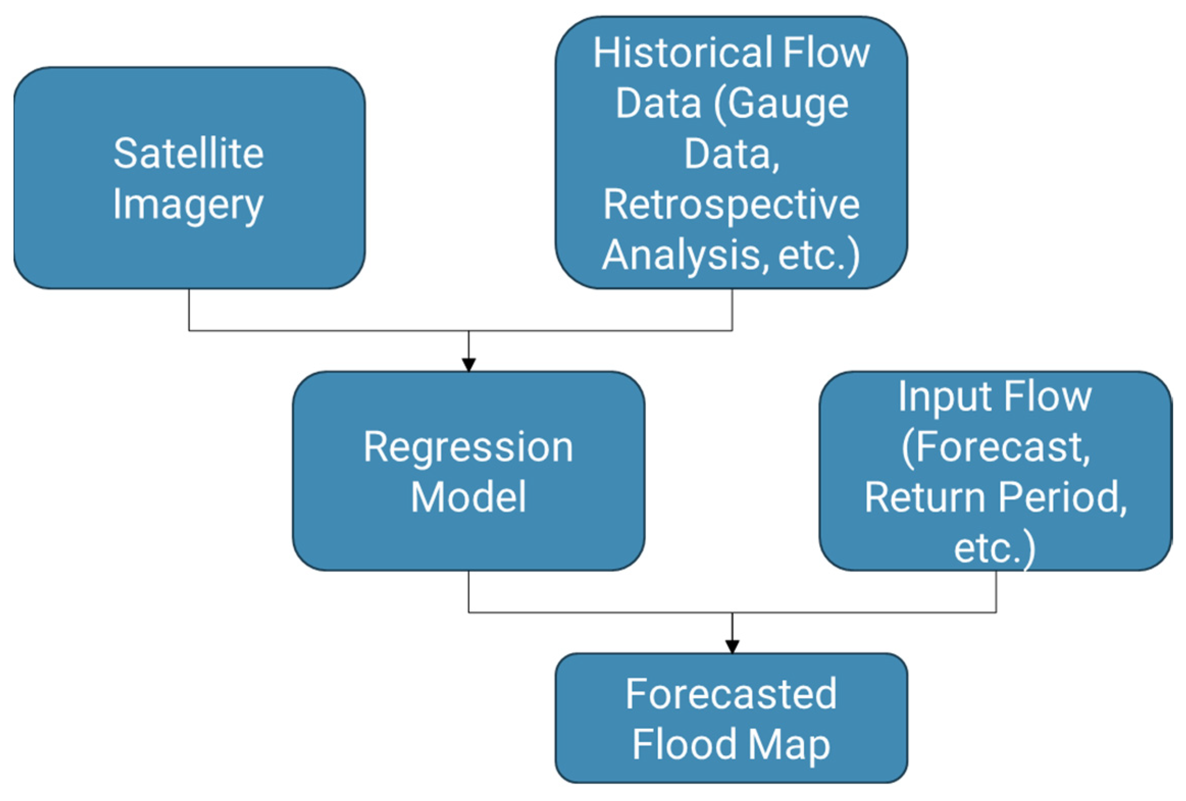
FIER forecasts flooding inundation maps (FIM) by first extracting spatial and temporal patterns of floods from historical imagery. The method correlates the observed flooding signal from satellite images with historical flows. It uses statistical methods to determine the discharge time series from gauges within a satellite scene that has the highest correlation with flood extents. It creates a regression equation that can use forecasted flows from the correlated station(s) and generate synthetic satellite imagery from the simulated flood signal combined with the spatial signals that can then be classified into a flood map. An overview of this process is shown in
Figure 1. Since this process relies on regression models and not on emulating physics as performed in traditional modeling, we will refer to the maps created by this and the other similar processes as synthesized or synthetic FIM. FIER was tested in the Lower Mekong, Tonle Sap Lake, the Lower Mississippi River Basin, and the Red River Basin [
13,
14,
15,
16,
17]. The methods are transferable because satellite observations are available worldwide, and either river gauges or global hydrology models can provide the discharge inputs.
1.2. Satellite Imagery
To satisfy the first requirement for a FIER model, we need satellite imagery of flooding events. Although satellite data are collected globally, they have several limitations that constrain their usefulness in flood mapping. Each satellite has a unique combination of distortions, and while methods exist to correct images, processing artifacts remain. Issues arise from atmospheric interference, cloud cover, backscattering, and topographical distortions [
18]. Both the spatial and temporal resolutions of the sensor affect the likelihood that a given flood is observed and that the detail captured will be sufficient to delineate the flood event. Many satellites have only been collecting data for the last several years or decades and have not captured many flooding events.
1.3. Flow Data
The original development of FIER models was generated using gauge data [
15,
16]. In this paper, we considered various large scale hydrologic models to fulfill the requirement of flow data [
17]. By including modeled data, we hope to remove the spatial limitation that gauges present. The sources for flow data include the GEOGLOWS Hydrologic Model and the United States NWM.
1.4. Research Objectives
To determine which locations are viable for satellite-based flood mapping, we created FIER test cases using GEOGLOWS and NWM data. This allows us to evaluate the theoretical implementation of satellite-based FIM at the global level. In this study, we will evaluate areas that are suitable for satellite-based models using Synthetic Aperture Radar (SAR) imagery from the Sentinel-1 satellites and Visible Infrared Imaging Radiometer Suite (VIIRS) optical imagery from the Joint Polar Satellite System (JPSS). We created suitability processes to determine the locations that have flood events that were captured in satellite imagery and, therefore, were likely suitable for model creation. We created separate processes for VIIRS imagery and SAR imagery. Once we categorized locations using these processes, we generated FIER models for locations in each category to evaluate the effectiveness of the categorization tools. These categorization processes can then be used to infer which locations are generally most suitable for satellite-based FIM.
2. Materials and Methods
2.1. Data
2.1.1. SAR Imagery
The Sentinel-1 satellites were designed and launched by the European Space Agency. The two satellites were equipped with SAR sensors whose imagery depends on satellite movement, and the images are marked as being collected during either the ascending or descending collection paths. The imagery can be used for forestry management, ice, oil spill and ocean monitoring, and flood mapping. The first satellite, Sentinel-1A was launched in 2014, and the second, Sentinel-1B, followed in 2016. Sentinel-1B ceased to function on 23 December 2021. Sentinel-1A has also exceeded its design lifetime and could cease providing data at any time. Plans to replace Sentinel-1A and Sentinel-1B with Sentinel-1C and Sentinel-1D have been delayed several times [
19,
20,
21].
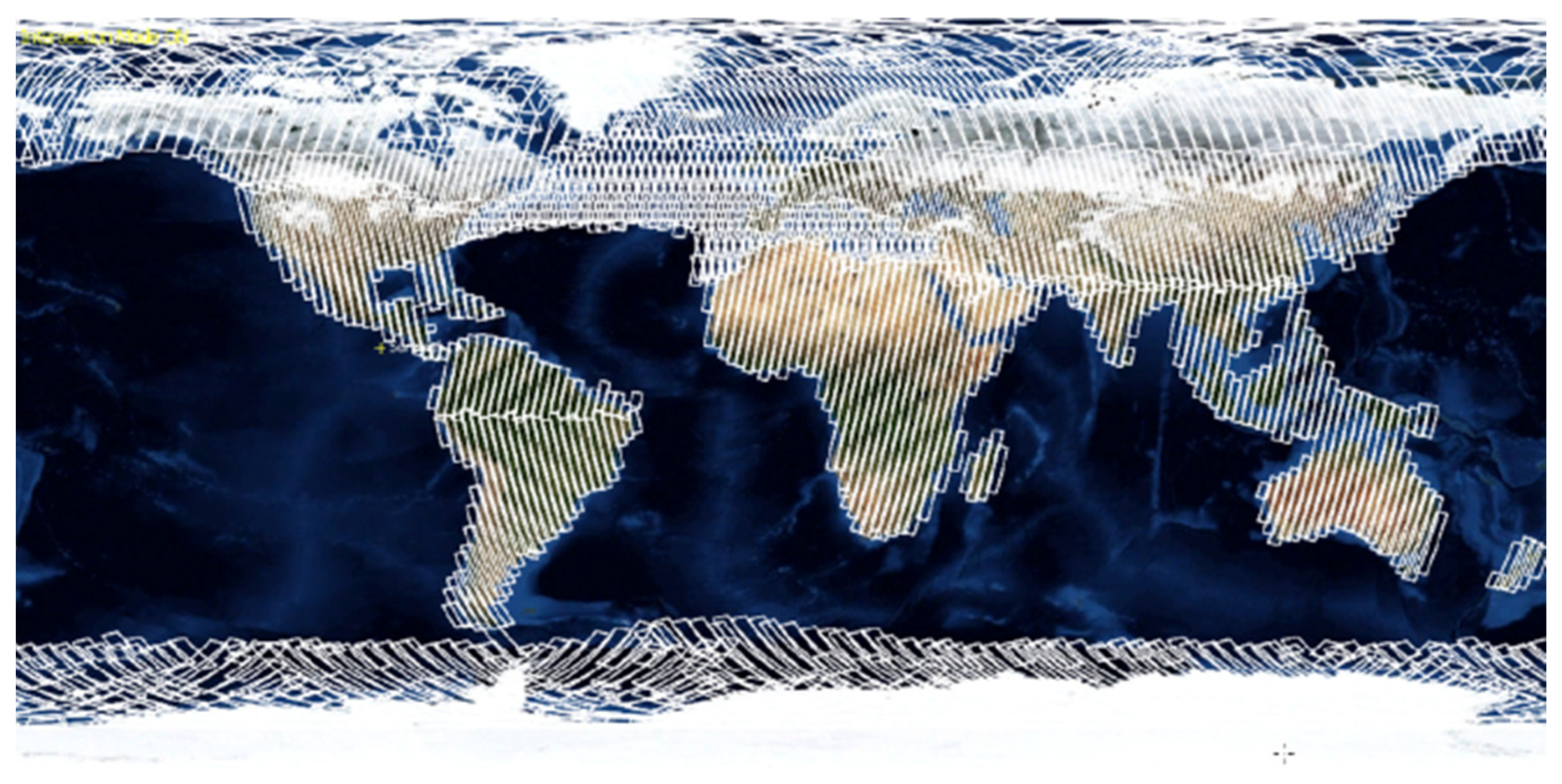
The resulting SAR images from the Ground Range Detected product have a 10 m resolution, which makes it possible to observe flows and floods on smaller streams and in smaller flood events. The main limiting factor is the revisit time of the Sentinel satellites. Because the satellites are in a polar orbit, the swaths are adjacent to each other at the equator and converge to a point at the poles, as demonstrated in
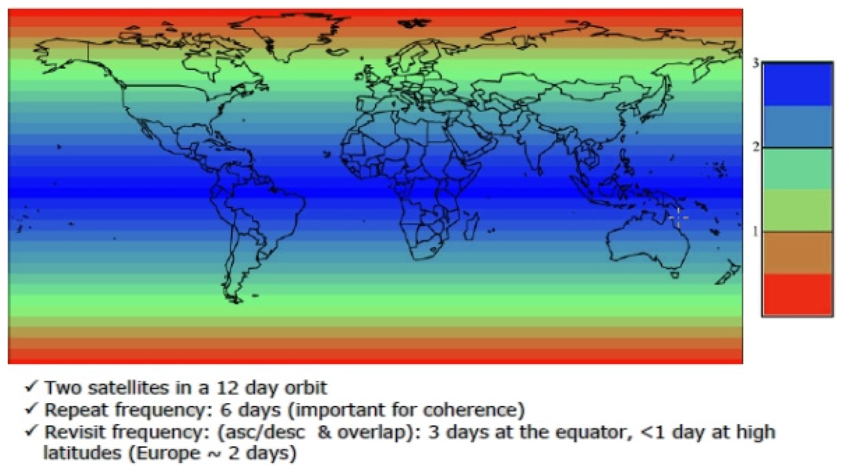
Figure 2. This means that any given point can be imaged in multiple swaths and that locations closer to the poles are imaged more frequently. The polar effects on revisit time are shown in
Figure 3. This figure is based on the theoretical coverage of the satellites when both were in orbit.
These figures indicate images will be collected at least every three days for any location on earth for both the ascending and descending orbits. However, data in
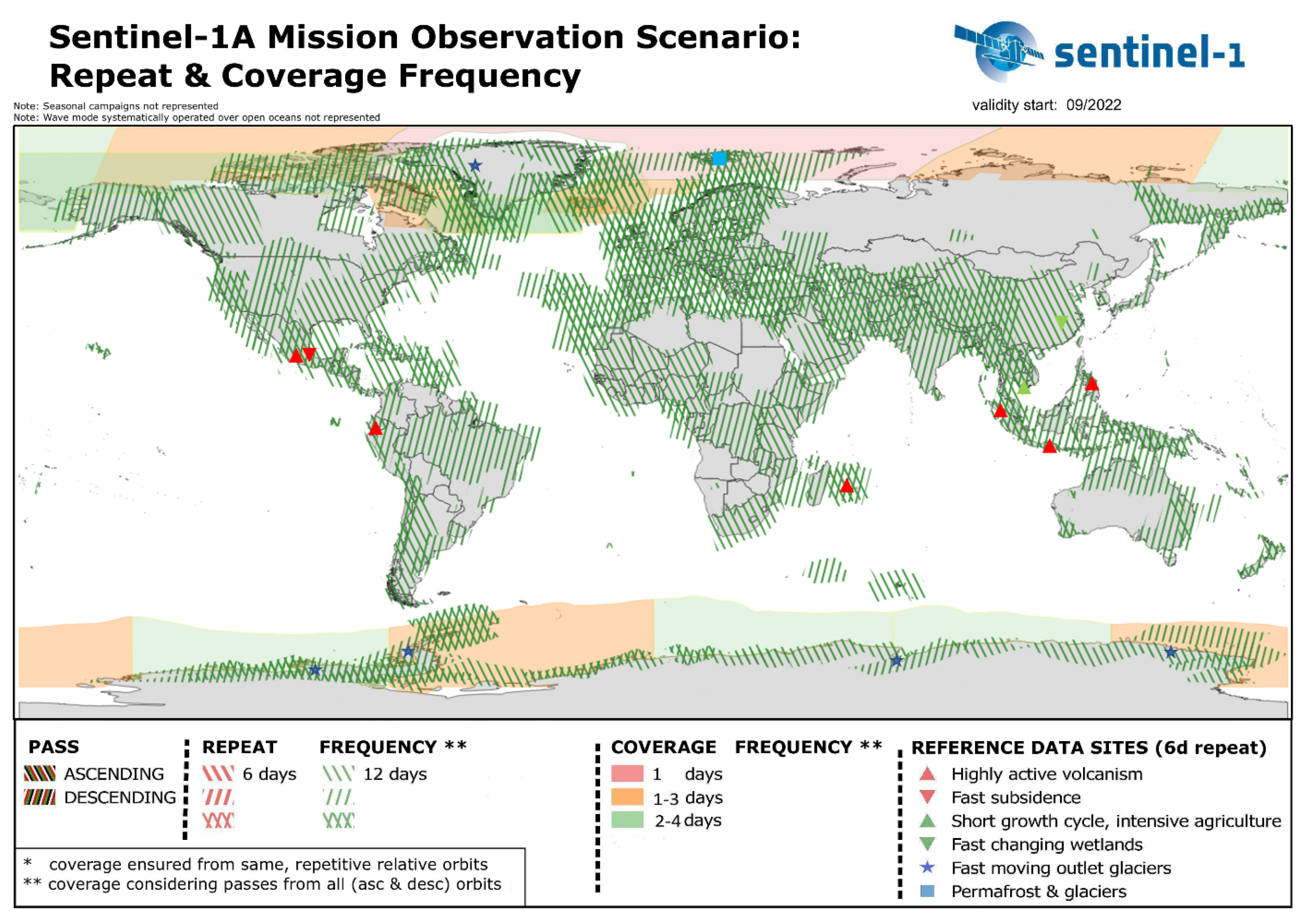
Figure 3 are not accurate because each satellite is limited to 30 min of IW band capturing each orbit. Instead, each satellite is tasked to complete a series of discrete missions over predesignated segments. The satellites prioritize Europe and with the failure of Sentinel-1B, no longer have enough coverage to image the entire globe.
Figure 4 shows the operational collection plan since the failure of Sentinel-1B. Notably, several regions of the globe no longer receive any images. While documentation is not readily available for Sentinel-1A’s mission observations plan before the launch of Sentinel-1B, the coverage would have been comparable [
22].
Because SAR is active remote sensing, it has some unique problems not found in passive remote sensing. Geometric distortions occur based on the angle at which the radar is beamed at the ground. Foreshortening makes hills slanted toward the sensor look shorter than hills slanted away from the sensor. In cases where the slant is steeper than the angle at which the beam is fired, this can lead to radar shadow and layover, where the back of a steep mountain is not imaged, and the valley behind the mountain appears adjacent to the peak [
23]. For example, foreshortening can be corrected using a DEM, but radar shadows cannot be filled [
18]. Active remote sensing is also prone to radiometric distortions. One example is speckle noise, where the random bouncing that occurs creates variation in intensity over the same surface. There are algorithms for correcting for this noise [
24,
25]. Last, SAR imagery relies on the specular reflectance of open water for detection, which can lead to errors of commission, with large areas of pavement or dry sandy soils being mistakenly classified as water [
26].
2.1.2. Optical Imagery
The National Oceanic and Atmospheric Administration (NOAA) operates the JPSS constellation of satellites launched in 2011, 2017, and 2022, which are equipped with VIIRS sensors that capture optical imagery. Because the VIIRS sensors cannot penetrate cloud cover, they often have missing information, especially during flood events. NOAA used the VIIRS imagery from the three satellites to produce an operational daily surface water fraction estimate for the entire globe [
27] titled NOAA JPSS/VIIRS Flood Mapping (VFM) product. The VFM imagery is equally to or more accurate than comparable products such as the Moderate Resolution Imaging Spectroradiometer (MODIS) for flood mapping [
28]. A water fraction map can be more useful than a classified flood map (i.e., each pixel is classified as either flood or not flood) because we can assume flood water occupies the fraction of the pixel with the lowest elevation, so we can use a Digital Elevation Model (DEM) to approximate sub pixel resolution flood extent [
12,
14,
29,
30,
31].
2.1.3. Properties and Limitations of Satellite Data
The key elements of the JPSS and Sentinel satellite systems are summarized in
Table 1. The JPSS VIIRS images capture the entire earth at least once a day; however, the optical sensors mean that not every image will contain a complete picture because of cloud cover and other atmospheric issues. In addition, the coarser spatial resolution of the VIIRS images, 375 m, means smaller streams are not visible in the imagery. To determine where VIIRS images are suitable for FIER modeling, we need to determine where water is visible on a pixel basis. Sentinel-1 SAR and JPSS VIIRS data were chosen specifically because of their previous applications with the FIER method. This combination of data is not the only set of options available. Many water mapping methods use other sources of optical or SAR.
The finer spatial resolution of the SAR images, 10 m, allows for much smaller rivers and flood events to be imaged. The SAR sensors mean that every image is complete, even on cloudy days. Because the Sentinel SAR sensors do not have continuous global coverage and a much less frequent revisit time, to determine where SAR images are suitable for FIER modeling, we need to determine which areas have been imaged when flooding occurred.
2.1.4. Stream Gauges
In-situ gauges that collect water level information combined with an updated rating curve are the most reliable source of streamflow data and are preferable to simulated historical data [
14]. However, there are several challenges associated with obtaining accurate gauge observations. Manual gauges are often recorded infrequently and can have large gaps in data, including periods during and after extreme floods where the gauge might have been destroyed [
32]. Each gauge has a different record length and rating curve data must be continually updated and calibrated to convert water level to streamflow accurately [
33]. There is bias in the placement of gauges on the global scale, meaning certain regions or river reaches are less likely to have gauges [
34]. The biggest limitation of gauge data is that they are not available globally or even for every stream reached in the US.
2.1.5. GEOGLOWS
The GEOGLOWS retrospective simulation provides the daily average river discharge from 1 January 1940 to the present for 7 million stream reaches. This means that consistent daily flow values are available globally. The retrospective flow values are currently limited to a daily average value. Theoretically, if a suitable satellite image is captured for a stream on a day when these hydrology data show high flows, there may be an offset between the daily average flow and the actual flow that occurred at the time of the image capture [
14]. The flow difference may or may not impact the accuracy of the synthesized FIM, and the significance of any error may plausibly vary for each river’s terrain, the number of useful satellite acquisitions at the river, the synthetic FIM generation method, the specific flow being predicted, and other potential error sources. Quantifying the effect would require site-specific analysis involving comparisons to observed flood maps which is out of scope for the general analysis we present here.
GEOGLOWS also offers average streamflow ensemble forecasts on the same 7 million river reaches at 3 hourly timesteps with a 15-day lead time. The forecasts provide 51 ensemble members with the forecasts updated daily. Regardless of which data are used to calibrate a FIER model, the GEOGLOWS forecast can be used as an input to FIER to estimate a forecasted synthetic flood map and its impact before it occurs [
35].
2.1.6. United States National Water Model
The NWM retrospective simulation covers the period from 1979 to 2020 with an hourly timestep. The NWM retrospective covers 2.7 million river reaches in the continental United States (CONUS) and is expanding to Alaska, Hawaii, and Puerto Rico. This retrospective provides hourly data on most of the rivers in the network. This increases the chances that the retrospective flow is close to the flow that occurred at the time an image was collected. The NWM also operates a streamflow forecasting system based on different meteorological forecasts, including the Climate Forecast System, which provides a lead time of 30 days, and the Global Forecast System, which provides a lead time of 10 days [
36].
2.2. SAR-Derived Synthetic Suitability Process
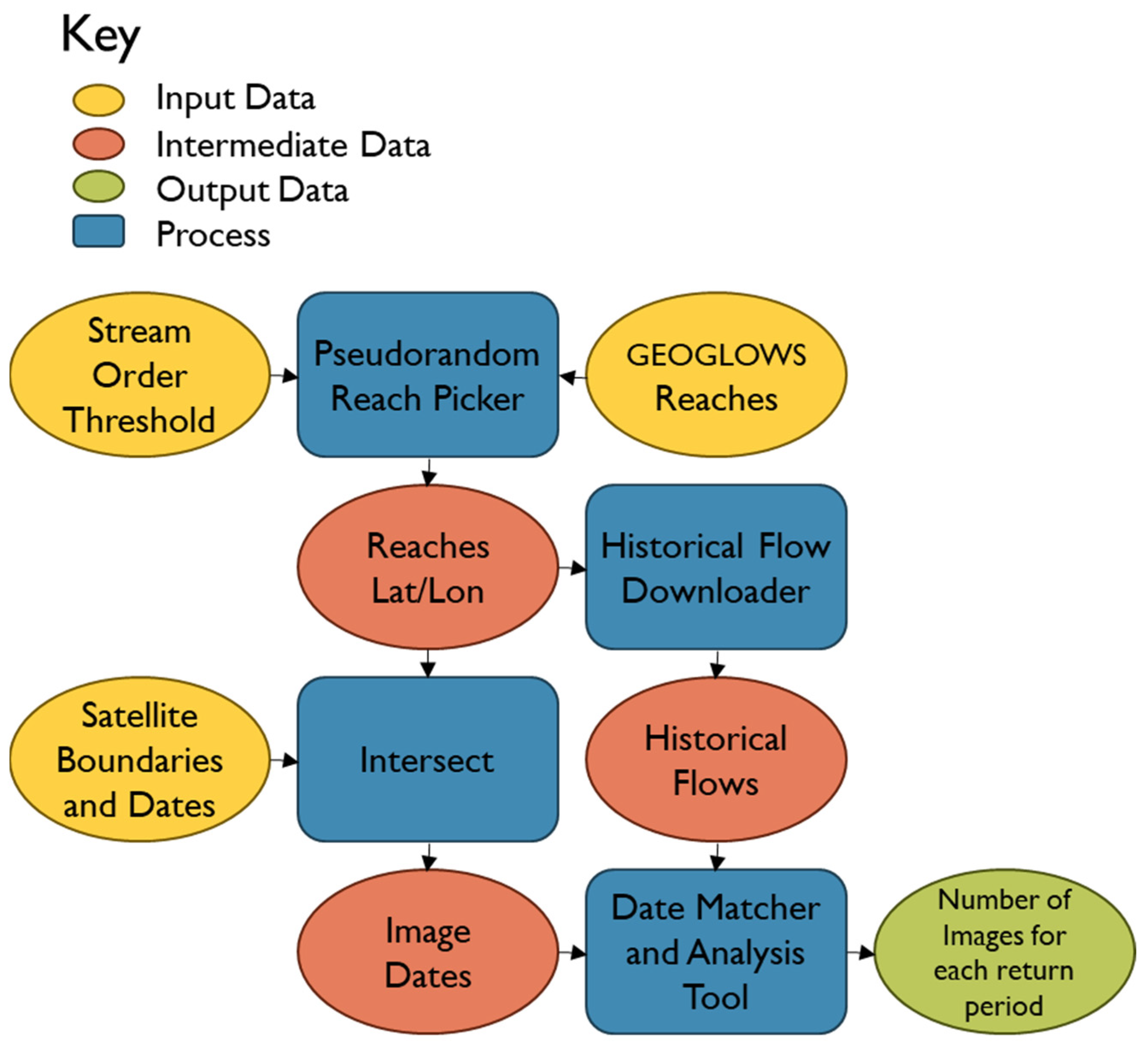
We evaluated which areas were suitable for SAR-derived synthetic FIM. A summary of this process is shown in
Figure 5. The biggest limitations with SAR are the revisit time and coverage; we need to identify which areas globally have been imaged while flooding occurred. Since determining flooding in SAR imagery requires extensive preprocessing, we instead identify areas with observed high flows, expecting many of them to be floods. We selected test areas around the world, and matched each image with the streamflow, then classified them into return periods. For exact locations, see the
Supplementary Materials. The return periods we used are less than 2, 2, 5, 10, 25, 50, and 100. From there we were able to determine the maximum return period that an area would be suitable for creating a SAR-derived synthetic FIM.
For our historical flow data, we decided to use the GEOGLOWS retrospective simulation because it is available globally. Because SAR has all-weather capabilities, we can assume that any image that is captured is complete and is suitable if the river is large enough to be detected. As a substitute for river width, we filtered the river reaches to Strahler stream order five or greater [
37]. Not all order five stream reaches have the same width, and some lower order reaches may be visible; however, for our purposes, we will assume they are visible. The GEOGLOWS hydrofabric contains nearly 7 million stream reaches based on the TDX-Hydro dataset [
38]. We lack the computational resources to analyze all these streams and need to take a sample of the global streams. We pseudo-selected streams with an order of five or greater. We ensured that the sampled streams were diverse in both location and stream order. This gave us a set of 4700 reaches to test that were spread across the globe on larger rivers. We downloaded the GEOGLOWS historical simulation, and the return periods for each of the sample river reaches.
For each of these sample reaches, we need to identify how many SAR images are available. The information we need for each image is the boundary, the time it was taken, and an identification number. Downloading only this information removes the need to store each image and decreases the processing time. We took the latitude and longitude coordinates of the centroid of each river reach and intersected them with the boundaries of the SAR images. We then labeled every image with the flow from the historical simulation for the day it was captured and classified it into a category based on the return period. We counted the number of occurrences of each return period at each location for each satellite pass.
To improve regression model accuracy, it is desirable to have data points at a range of flows to avoid large interpolations or extrapolations, which can lead to over- or under-fitting. FIER cannot extrapolate, so knowing the maximum return period class indicates the highest flow the model could synthesize based on the range of values available from the sample datasets. We assigned every reach into a category based on the maximum return period of flow that it had observed, with at least one observation in every preceding return period category. We looked at return periods for 2, 5, 10, 25, 50 and 100 years. We excluded any points that were inside of lakes using the World Wildlife Foundation’s Global Lakes and Wetlands Dataset [
39] because GEOGLOWS reports streamflow data for lakes, and the inundation around lakes is not a function of current streamflow.
Because GEOGLOWS does not account for control structures, we expect that many of the high flows that it predicted will be mitigated. Even under this assumption, the ratio of floods that were imaged is informative about the chances of observing low exceedance probability of high flows. To understand these patterns, we calculated the ratio of test locations that were classified as suitable for each return period.
2.3. VIIRS-Derived Synthetic FIM Suitability Process
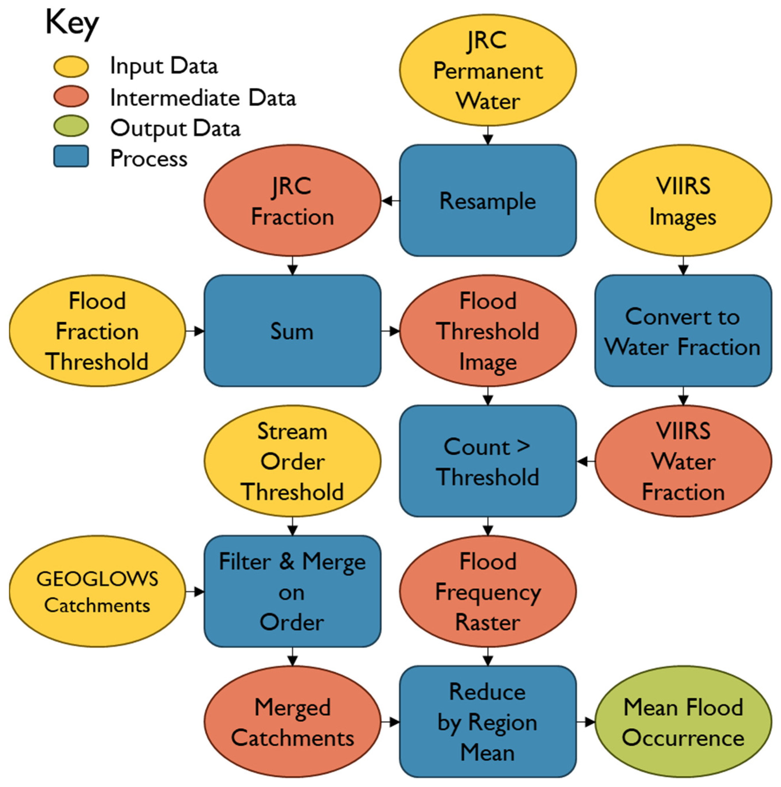
The process for determining suitability for VIIRS-derived synthetic FIM is shown in
Figure 6. The largest limitations of VIIRS data are the coarse resolution and some pixels that are masked by cloud cover. To determine which areas are suitable, we need to determine which areas have observed flooding. We must differentiate flooding from permanent water and then associate each area in the imagery with a stream segment. This allows us to calculate which streams have experienced the most flooding and, therefore, are most likely to be suitable for a VIIRS-derived synthetic FIM model.
The first step was to prepare the VIIRS images. We used the NOAA JPSS/VIIRS Flood Mapping Product [
28]. We downloaded these data from
https://jpssflood.gmu.edu/ (accessed on 1 January 2025) and the JPSS flood Amazon S3 bucket. For the scope of this paper, we only processed the images for the United States, Canada, and Mexico. We merged (mosaic-ed) the images (tiles) for each day into a single image. This resulted in 3529 daily images. The daily images contain classified pixels, including snow, ice, bare earth, and open water. It also includes water fractions for partial pixels. For our study, we changed the open water to represent 100% water and kept only the water fraction. Snow, ice, and bare earth are all considered 0% water, while clouded pixels are considered no data.
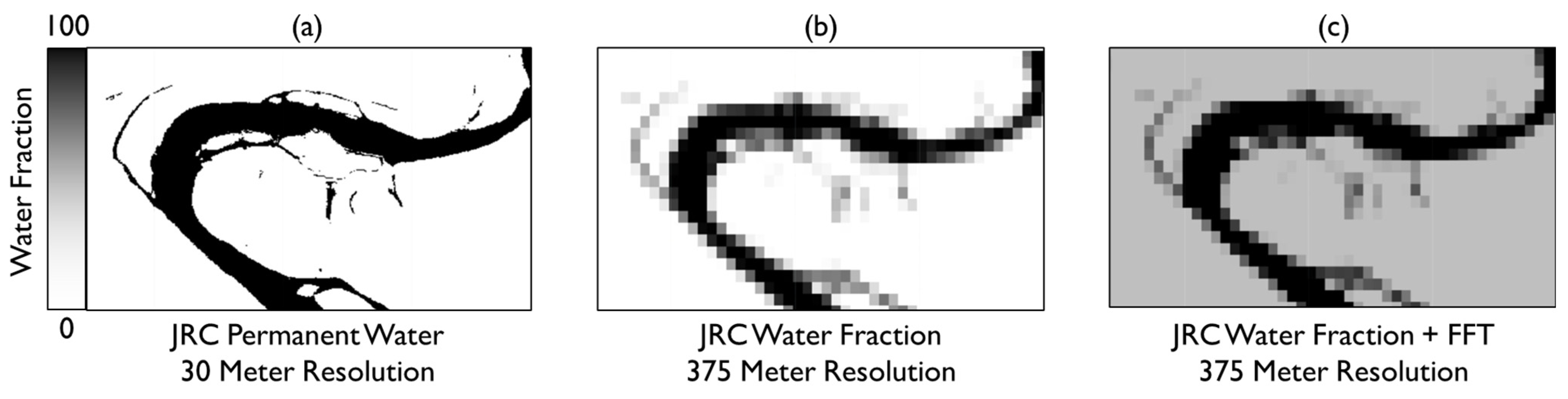
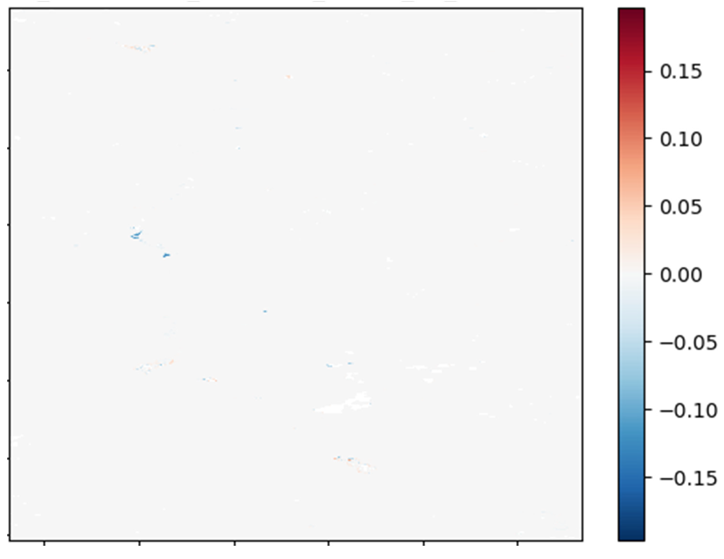
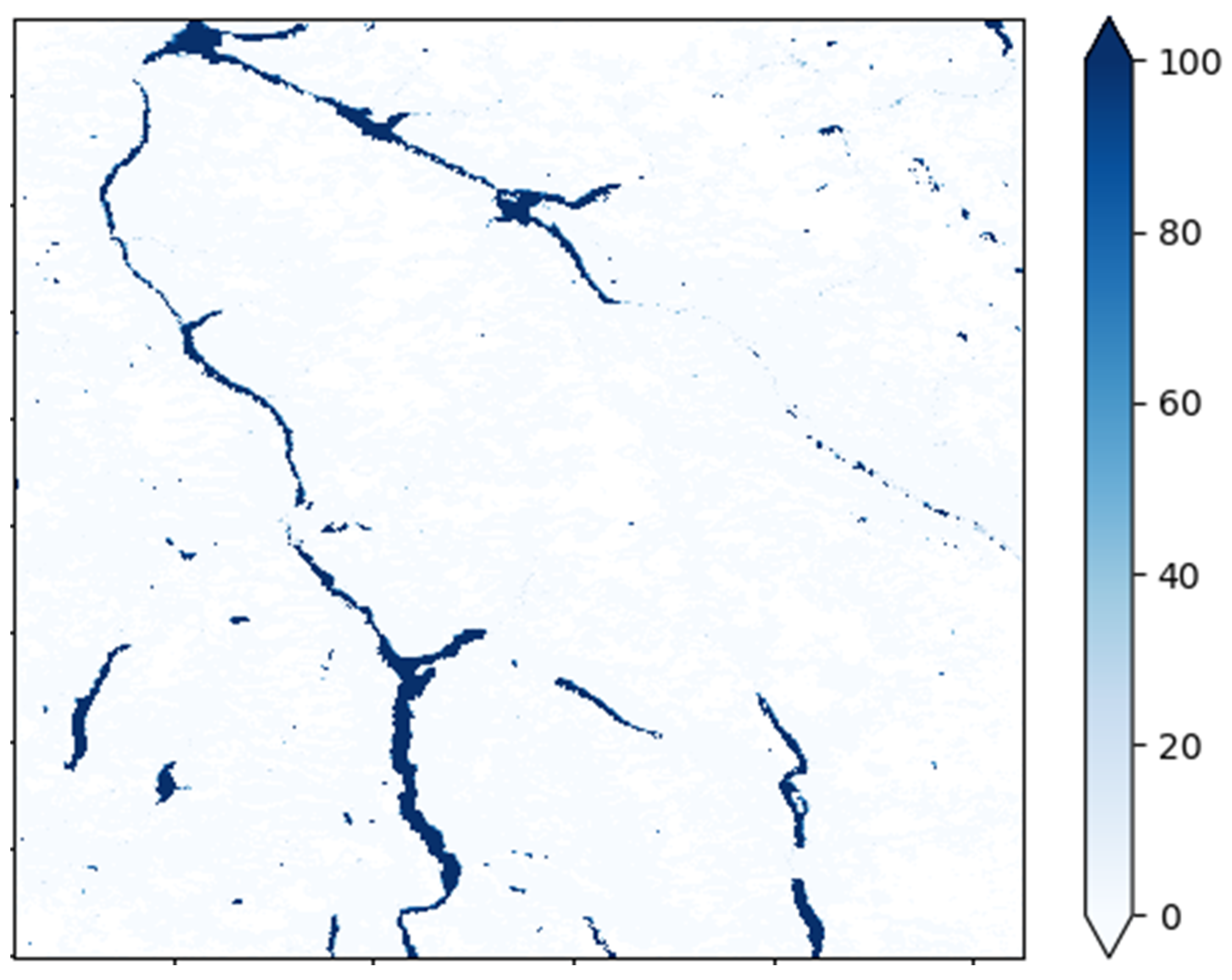
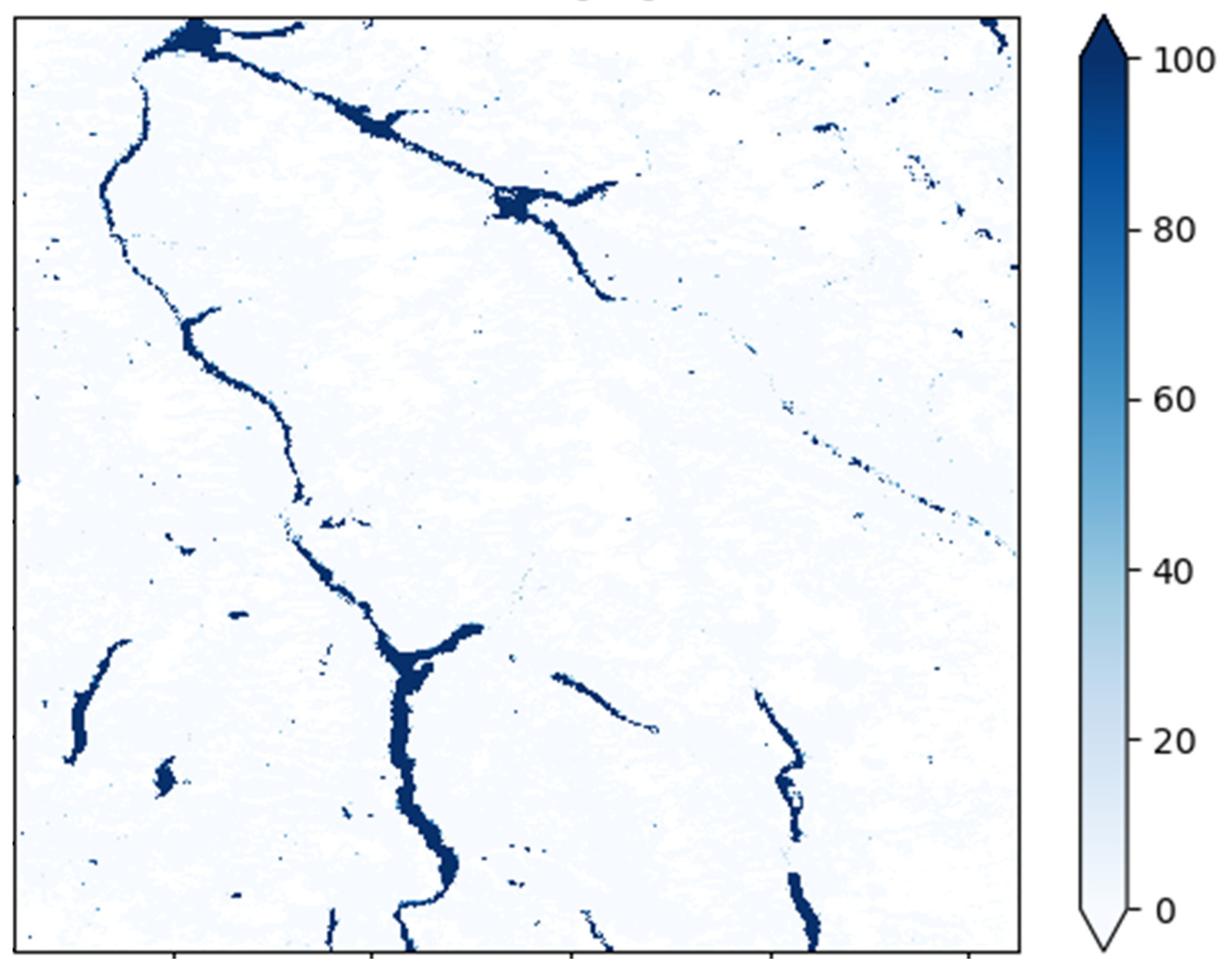
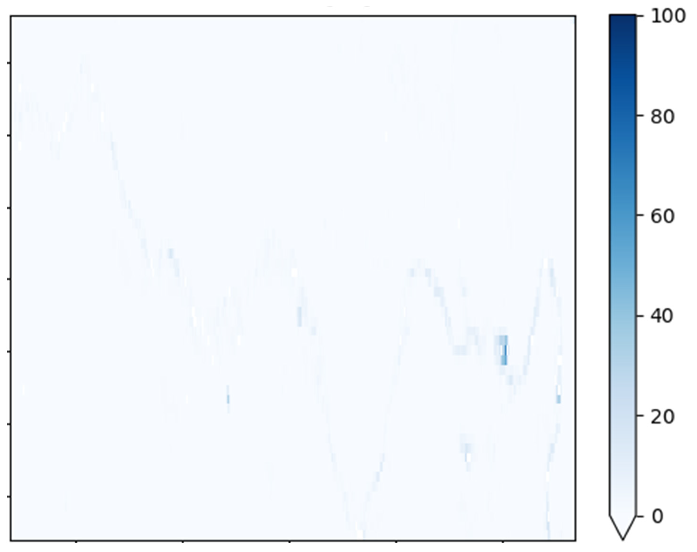
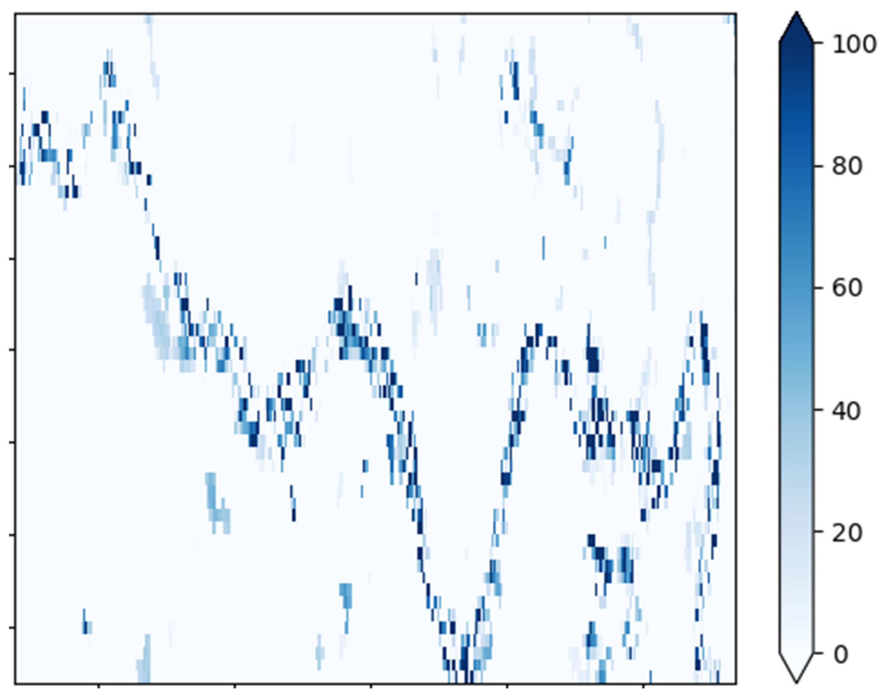
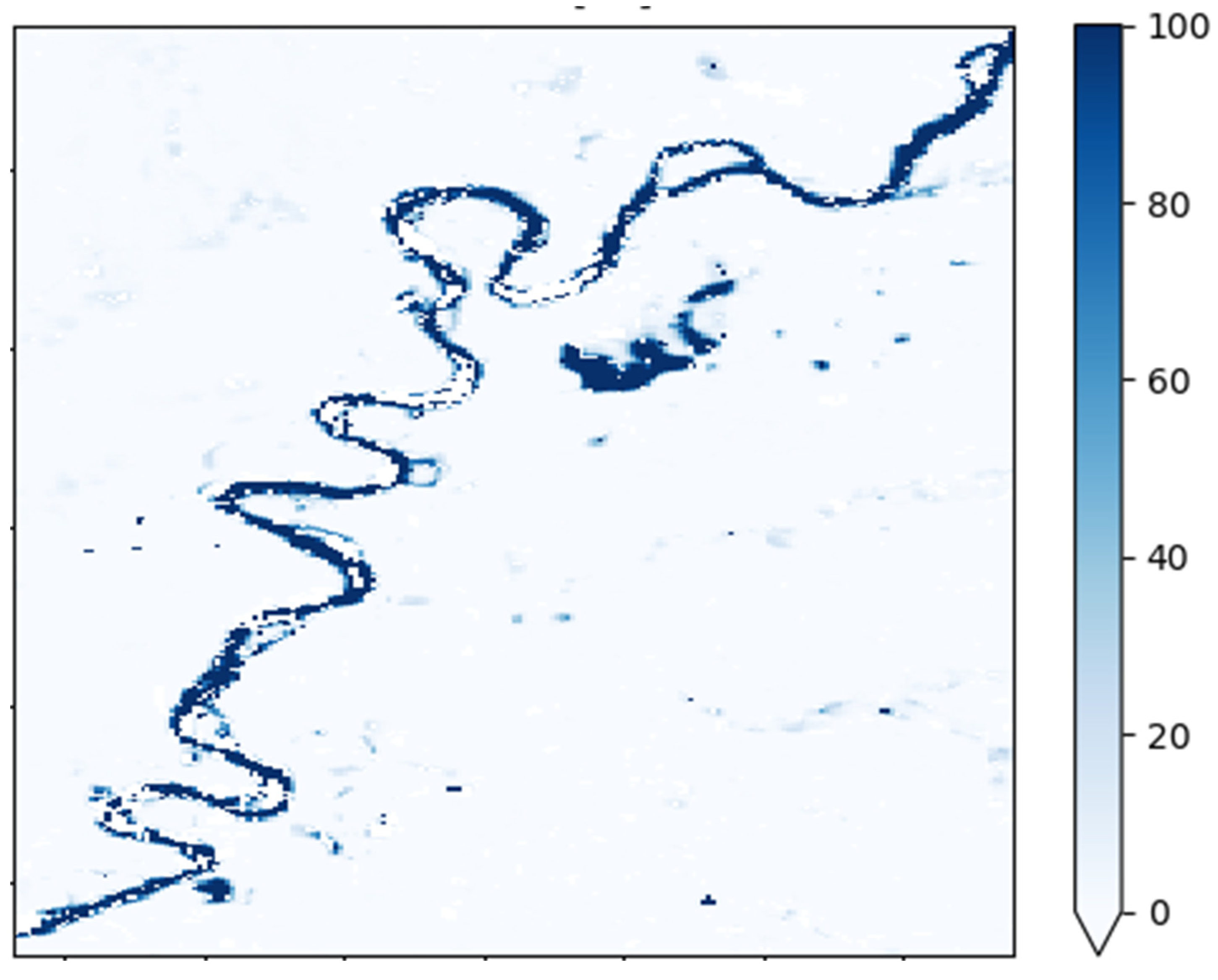
To differentiate flood water from normal water, we used the Joint Research Centre (JRC) Permanent Water dataset. This dataset contains categories for permanent water, including seasonal and permanent water, along with categories representing the change in permanent water from 1980 to 2000 and from 2000 forward. Because the period of our satellite images resides entirely within the “new” period in the JRC Permanent Water dataset, we extracted all the pixels with permanent water and set their values to 100 so that they were on the same scale as the VIIRS images. The JRC permanent water dataset has a 30 m resolution, which is much higher than the VIIRS imagery. An example of the high-resolution JRC Permanent water image is shown in the first pane of
Figure 7. To enable comparison with the VIIRS imagery, we resampled it to the VIIRS resolution by taking the mean of the JRC Permanent Water pixels inside of each VIIRS pixel. This converts it into the percent water fraction. An example of the resampled JRC image is shown in the second pane of
Figure 7.
By comparing the VIIRS images with the resampled JRC Permanent Water image, we can determine the water fraction for each pixel. Since we are interested in flood mapping, we would like to include only pixels that flooded. We assumed that flooding occurs when water is present in a certain fraction of the pixel above what it normally occupies. We will call this value the flood fraction threshold (FFT). Because we did not know what the FFT should be, we ran the process with FFTs ranging from 0% to 100% at 5% intervals. We added each FFT to the JRC Permanent Water Fraction image to create 21 flood threshold images. An example of a flood threshold image is shown in the third pane of
Figure 7.
To determine the frequency of flooding, we counted the number of times each VIIRS pixel exceeded the flood threshold image. We repeated this process for each of the 21 flood threshold images. For each FFT this gives us a raster where the pixel values represent the number of times each pixel is considered in flood conditions over the study period, in other words, the number of flood occurrences.
Because we are interested in which areas are suitable for VIIRS-derived synthetic FIM, we need a method of grouping the pixels from the flood frequency raster into model domains. We can accomplish this by using the GEOGLOWS catchments. Because small streams are unlikely to be detectable, we filtered the river reaches to Strahler stream orders of five or greater [
37]. These stream orders are subjective and depend on the resolution that the stream network is delineated at [
40]. We selected order five streams by visually inspecting images of several rivers in normal conditions to see what was detectable. Because a single GEOGLOWS reach is likely not large enough for a model domain, we merged all contiguous catchments of the same stream order into a single polygon. This yields about 12,250 areas that could be used for flood modeling, which, on average, was the aggregation of 11 GEOGLOWS river reaches.
We took the merged catchments and used a mean reduction by region for each of the 21 flood frequency rasters. This calculates the mean number of flood occurrences for each group of catchments for each of the rasters. We calculated the mean instead of the sum because the mean enables comparisons between catchment groupings of different sizes. The higher the mean flood occurrence for a group of catchments, the more flooding it has experienced, and the more likely it is to be suitable for a VIIRS-derived synthetic FIM.
2.4. VIIRS FIER Test Cases
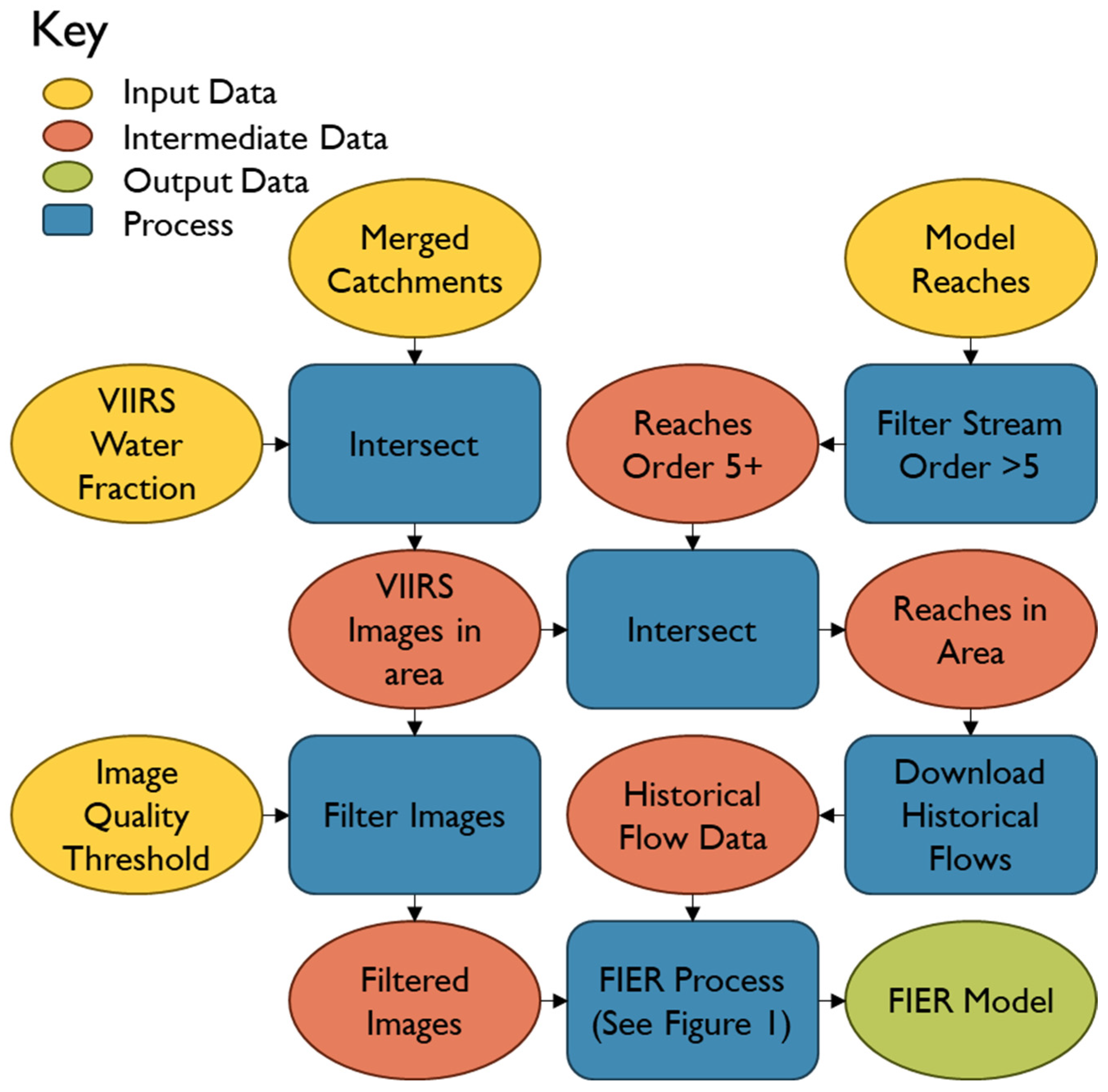
To inspect the effect of mean flood occurrence on the models that are generated, we created some test FIER VIIRS Models. A summary of the test case process is shown in
Figure 8. We selected 20 catchment groups from our study area with different mean flood occurrences, as determined by the suitability process, and from different locations. We attempted to generate a FIER model for each catchment. After each model was generated, we evaluated the performance of these models.
For each catchment group, we downloaded the VIIRS images that had been processed into water fractions. We clipped the images into the smallest rectangle that would contain the entire catchment group. By using a larger area than just the catchment groups, we include confluences and small portions of tributaries where flooding would likely occur if the mainstem is in flood conditions.
All pixels that have no data values in any image we use for calibrating the FIER model are removed from the final model. If we used the entire image collection, all pixels would be masked; if we use only images that are complete, we will likely not have enough images to calibrate the model. We need to establish an image quality threshold that filters the images such that there are enough images to calibrate the model and the images contain enough matching pixels that the final model is useful. Since we do not know what the optimal value is for the image quality threshold, we will calibrate models for a variety of values. We prepared sets of images for each catchment group for image quality thresholds 99.99%, 99.95%, 99.9%, 99.5%, and 99%, where each image must have at least that percentage of valid pixels to be included.
We use image footprints to identify the reaches from both NWM and GEOGLOWS and download historical data. This includes tributaries to the catchment groupings. As with the suitability process, we limit the stream reaches to those that have a stream order of five or greater. Because NWM does not report data on all its reaches, we must then remove any reaches that do not have historical data. We generated FIER regression models for each of the 20 catchment groups for both NWM and GEOGLOWS for each set of images (see
Figure 1).
Because there is not a single metric that accurately describes the performance of a FIER model, we took the resulting models and placed them into categories based on performance and types of errors. This allows us to see what types of errors are most common for different ranges of means. Because the models created from different image quality thresholds perform differently, the best-performing model was considered for each catchment group. Further, since we are not comparing the FIER outputs to observed flood extents and it is not the purpose of this paper to assess any synthetic FIM generation method, we will only qualitatively evaluate these maps.
3. Results
3.1. Differences Between SAR-Derived Synthetic FIM Suitability and VIIRS-Derived Synthetic FIM Suitability
The results for SAR-derived synthetic FIM suitability and VIIRS-derived synthetic FIM suitability measure different requirements of satellite-based flood mapping and investigate different spatial domains. The VIIRS-derived synthetic FIM suitability process examined about 12,250 catchment groups across North America. This was possible because once the VIIRS water fraction images were loaded into GEE, minimal processing was required to convert the images into water fractions and determine which pixels were considered to be flooding. The coarse resolution of VIIRS makes reducing the images into a flood frequency raster fast. If this same procedure were conducted with SAR imagery, the images would have to be processed in batches because the image collection exceeds GEE’s maximum storage space. The preprocessing to filter speckle and terrain distortion would require the selection of a DEM. Identifying the water pixels would require thresholding or the use of an existing water classification package. Once flood pixels were identified, the 30 m resolution of the images would make the resulting flood frequency raster around 150 times the size of the VIIRS version for the same study area. All these factors make performing this analysis for SAR at the global scale prohibitively time-consuming.
Consequently, for the SAR imagery, we assumed that each image was complete and used the footprints and historical flows to determine the return period of the flow that was imaged, assuming that higher return period flows are more likely to flood. If this same assumption were applied to the VIIRS images, the maximum flooding observed would be equal to the maximum flooding on the river since an image is recorded every day, and many of the images would be completely blank or masked. This could be avoided by filtering for only complete images, but because the images we processed into GEE are one image per day, none of them would ever be complete. The images would need to be divided into smaller chunks and then filtered, which would require significant processing.
Because such different processes must be used, our analysis does not support conclusions suggesting either VIIRS or SAR is superior for synthesizing FIM. The VIIRS results present general suitability based on observed flooding for each group of catchments over North America. The SAR results present the maximum imaged return period of flow at discrete locations sampled across the globe. The results for both methods must be understood separately and weighed against the advantages and disadvantages of each, and the characteristics of the area where a flood model is to be developed.
3.2. SAR-Derived Synthetic FIM Suitability
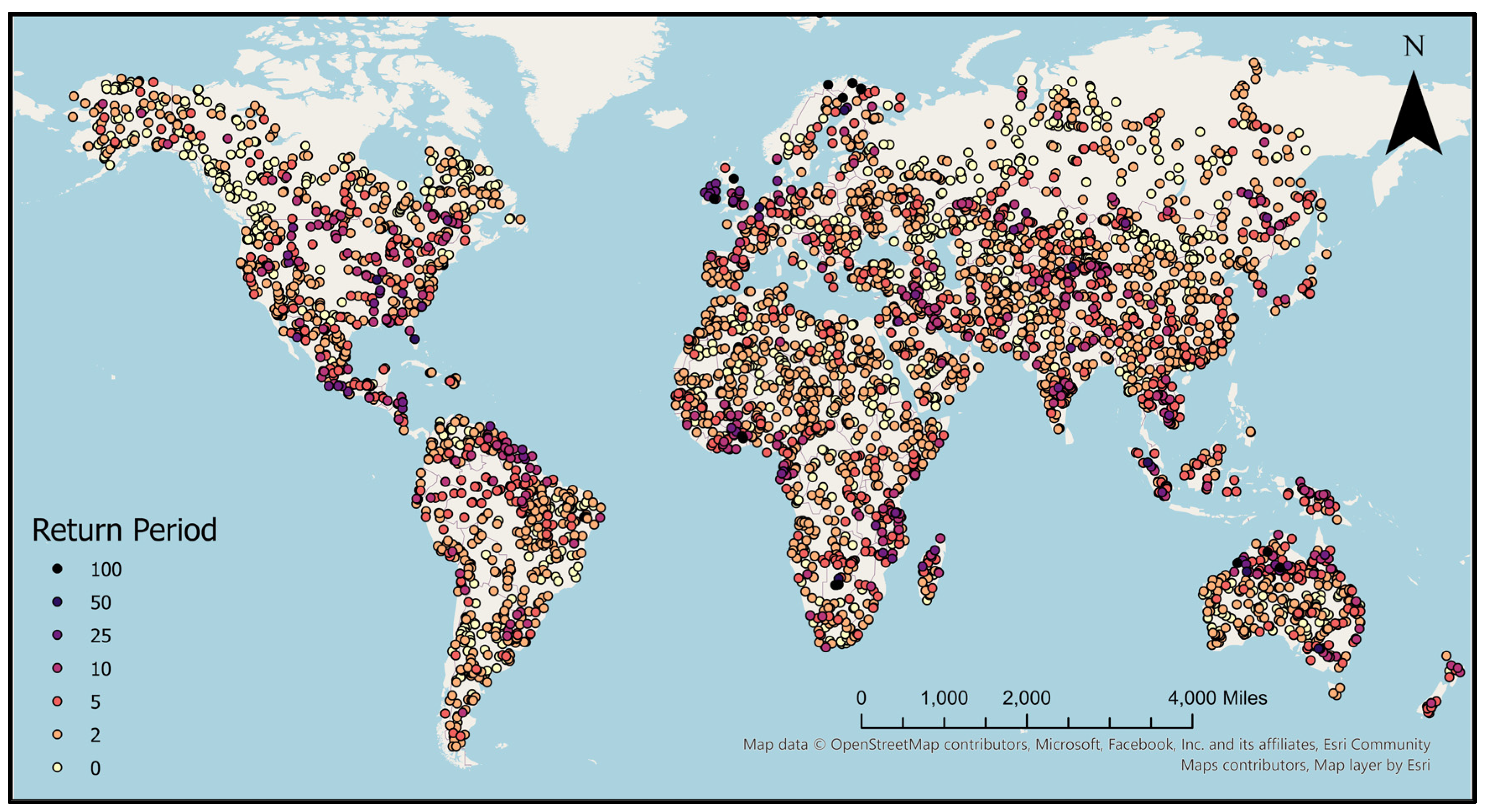
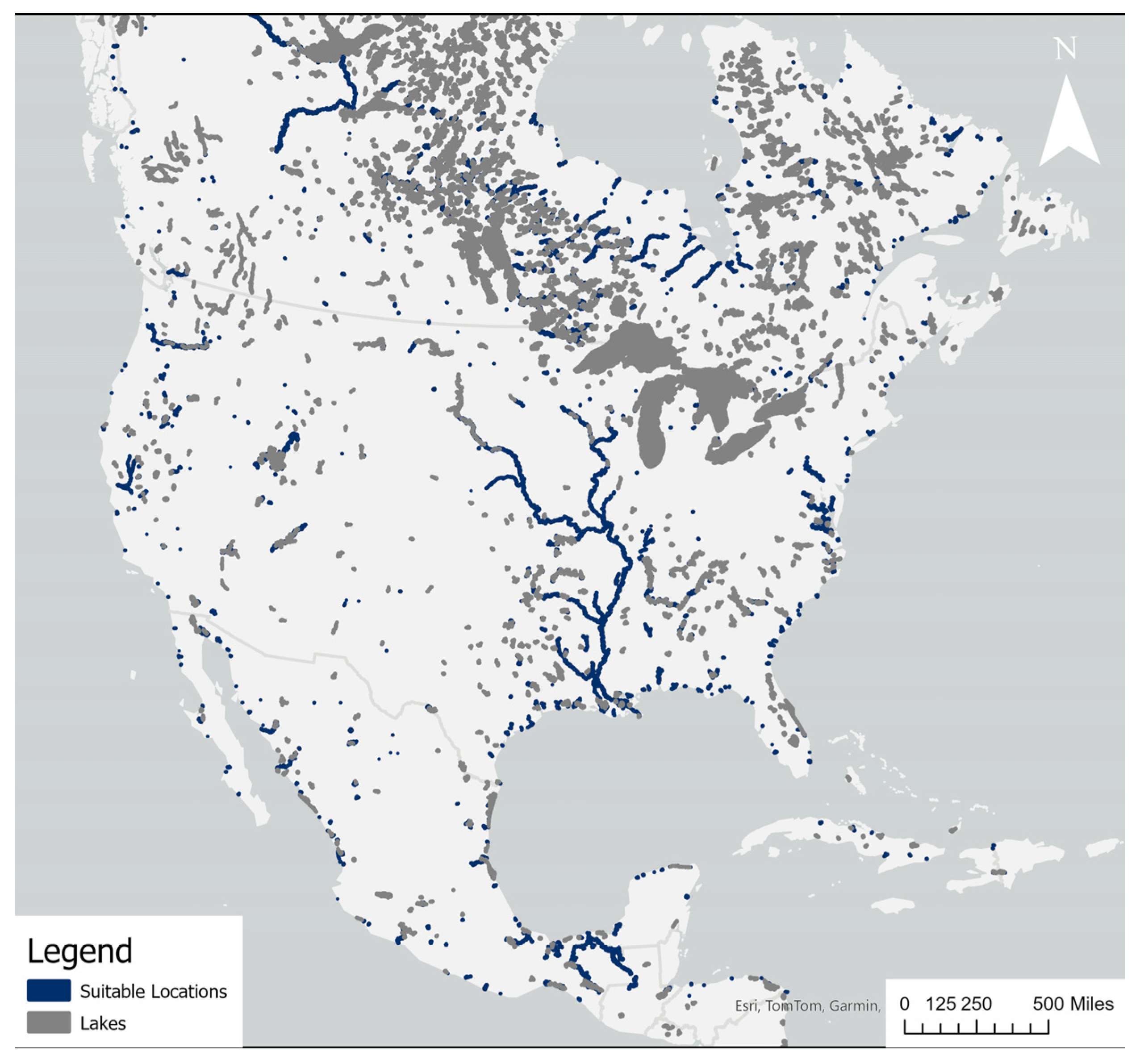
The maximum feasible return period for a satellite-based model with SAR for each of the over 4700 reach IDs we evaluated is shown in
Figure 9. The source geospatial dataset for this figure is available in the
supplementary materials. This map takes the highest feasible value calculated from both the ascending and descending passes. The maximum feasible return period may not be the highest imaged return period because we want at least one data point for return periods along our range of flows. Detailed numbers for the number of images classified into each category for both the ascending and descending passes, along with the statistics for the maximum values and the percentage of points in each category, are shown in
Table 2.
Areas without any test reaches are either areas where GEOGLOWS does not report data, such as Greenland, or areas where all the streams are less than stream order five, such as the central US. Rivers that regularly overflow their banks may be feasible for the generation of FIER models at much lower return periods than rivers that only overflow their banks in extreme events. Similarly, arid areas have low thresholds for 100-year events and still may not have been visible to the satellite or overflowed the banks despite the large return period. This applies to the high return period points in Australia. As more data are collected, more points will become suitable for models of higher return period flows.
From our test cases, more areas were imaged on the descending pass than on the ascending pass. The majority of images, about 72%, were suitable for a 2-year return period or less. Less than 2% of all our test cases were suitable for anything higher than a 10-year return period. The areas that were classified as suitable for a 100-year return period totaled only 0.32% of the test cases, making them very rare. Across all return periods, these probabilities are much lower than the probabilities of floods occurring in these return periods within approximately ten to fifteen years of available observations (
Table 3).
We did not exclude from consideration any areas which are not being imaged at present. It may be possible that those places are suitable with relatively fewer years of satellite images available. The points that are classified into the higher return period suitability, shown in
Figure 9, mostly lie in the area that has continued to be mapped, as shown in
Figure 4. That suggests that areas that were only imaged before the failure of Sentinel-1B do not have enough images to be useful for synthesizing FIM. Therefore, the first step in determining an area’s suitability for a satellite-based model with SAR imagery is to determine if it is still being imaged.
Further evaluation would include checking to ensure that the river is detectable. Our methods do not account for any possible interference from mountain ranges or urban environments. Our methods do not account for any limitations in the hydrological models. For example, the GEOGLOWS hydrologic model does not account for control structures. This means that any water that enters a river is routed to the end, even if a dam is present. This can create high return period flows in the model that, if imaged, would register as suitable for flood model creation but do not contain any flood. Therefore, some of the locations that have been classified as suitable may not be. Regardless, the ratio of areas tested to areas that had experienced high flows provides insight into how likely it is to capture enough images of high flows in an area.
3.3. VIIRS-Derived Synthetic FIM Suitability
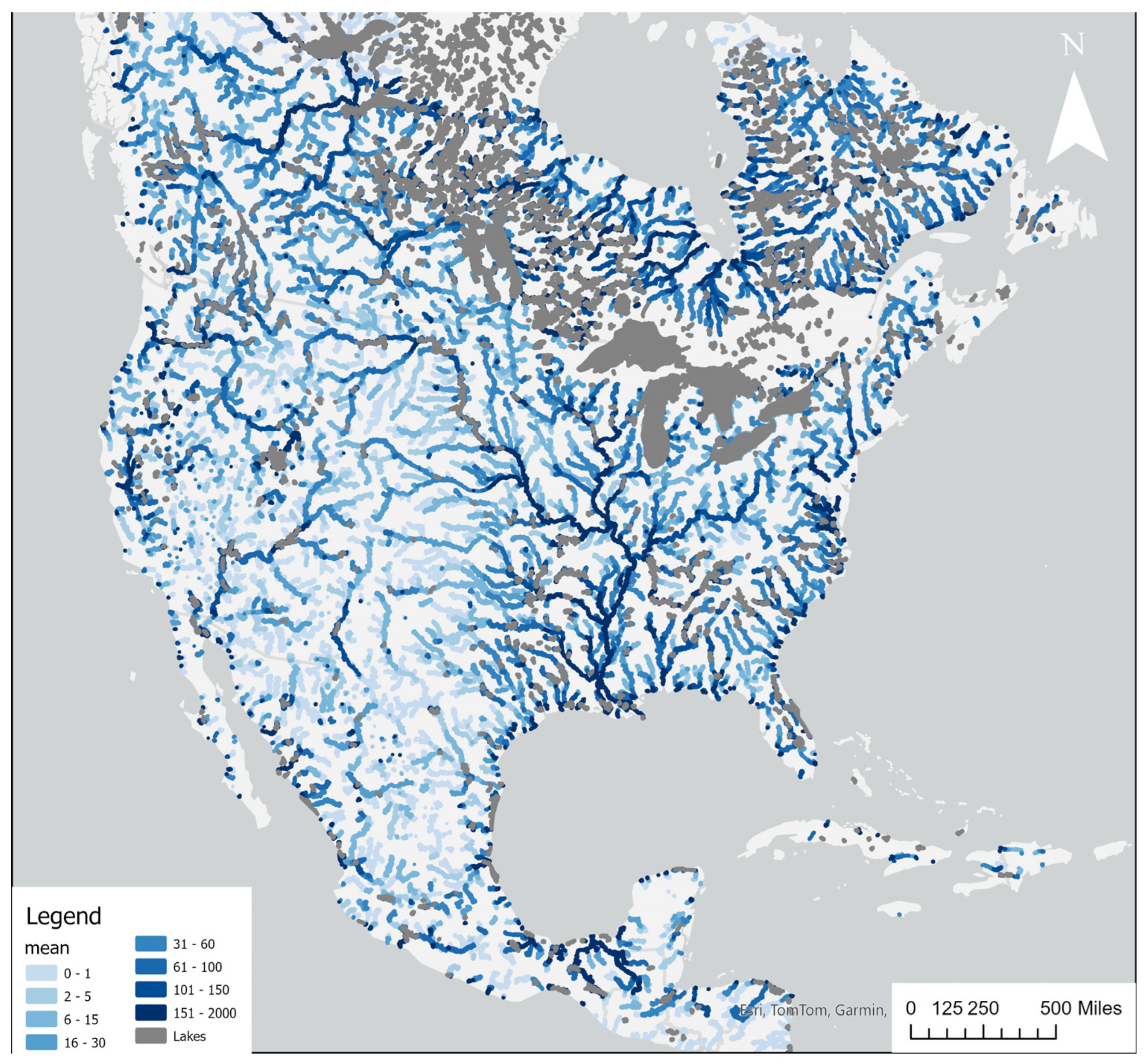
We computed the mean inundation observation for every water fraction threshold. The results for the 25% threshold are shown in
Figure 10. We chose 25% because it excludes minor water bodies and minor flooding; lower thresholds all provide similar results. The maps for the other FFTs are available in
supplementary materials. The highest thresholds provide errant results because any pixels with any permanent water cannot be counted as flooding, even if they are completely inundated. The darker the blue of an area shown in the figure, the higher the mean inundation observation across the catchment. Areas with a higher mean are likely more suitable for satellite-based models. Lakes where the flow does not control the inundation are masked in dark gray. Because this method works by counting pixels, an area that shows a lower mean may still be feasible for a satellite-based model if several large events were observed.
3.4. FIER VIIRS Case Studies
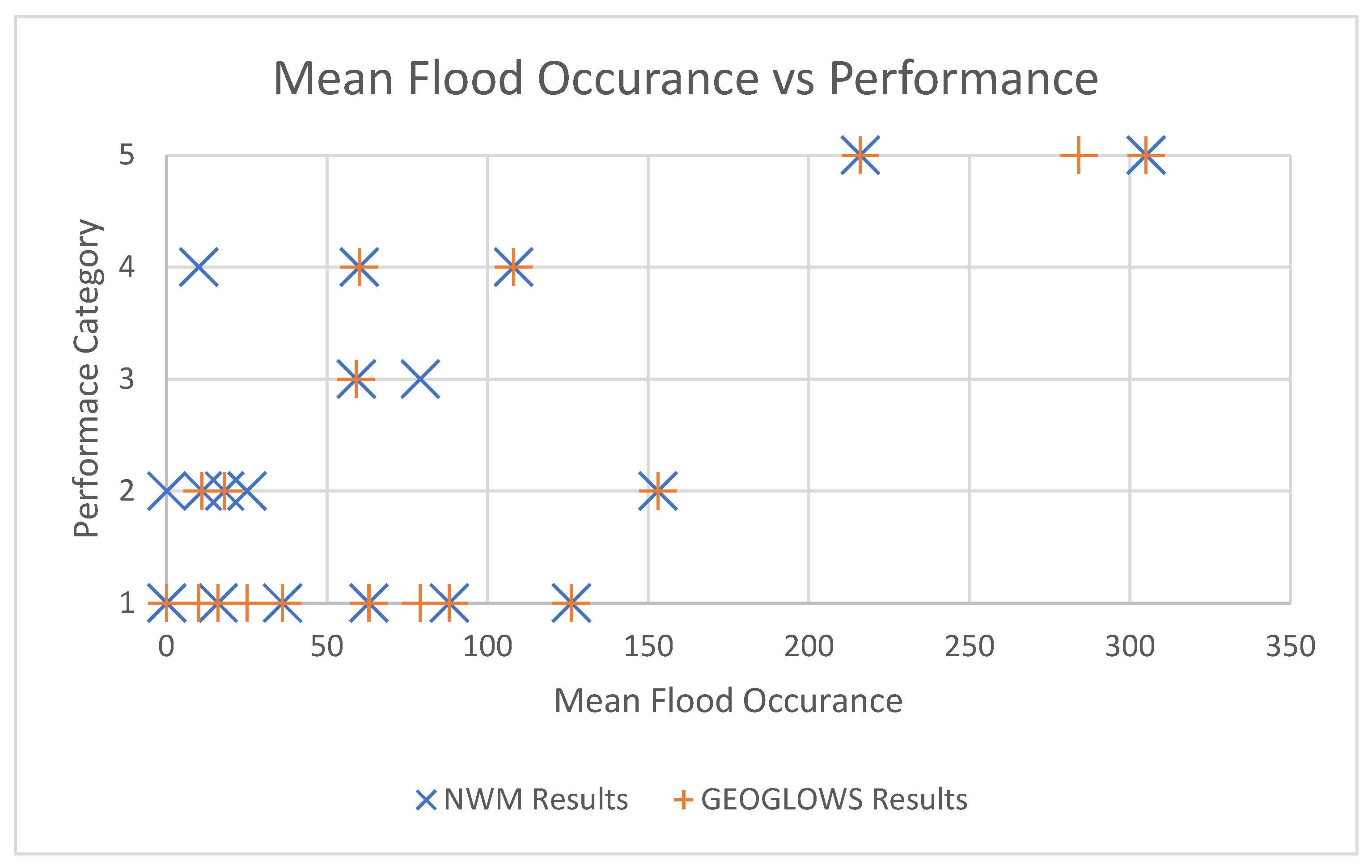
We built 20 FIER models to test the effect of mean flood occurrence, as shown in
Figure 10. The results from our case studies are shown in
Figure 11. A table of values with additional labels is given in
Appendix A. We evaluate the 20 models, looking for categories of errors or skills that are present compared with the range of data used to create the model. We found the first category was for models where no significant correlation was found, meaning these training data were insufficient for the FIER method. From the remaining models, we examined the spatial mode to see which areas it identified as changing. Models exhibiting only noise and no discernable patterns resembling the permanent water were labeled Category 2. For the remaining models, we input historical flow data from the highest flow month and the lowest flow month to synthesize flood maps (see
Figure 1). After visually inspecting each of the maps, we categorized any models that did not change from the highest flow month to the lowest flow month as Category 3. Category 4 represents models that change from low flow to high flow, but the change is from displaying nothing to displaying some river features, meaning the river is only wide enough to be detected in high-flow scenarios. Category 5 was for models that exhibited a spatial pattern consistent with the permanent water mask and, therefore, are considered to work as well as FIER is capable for that scenario. Example figures of models from Categories 2 to 5 are given in
Appendix A.
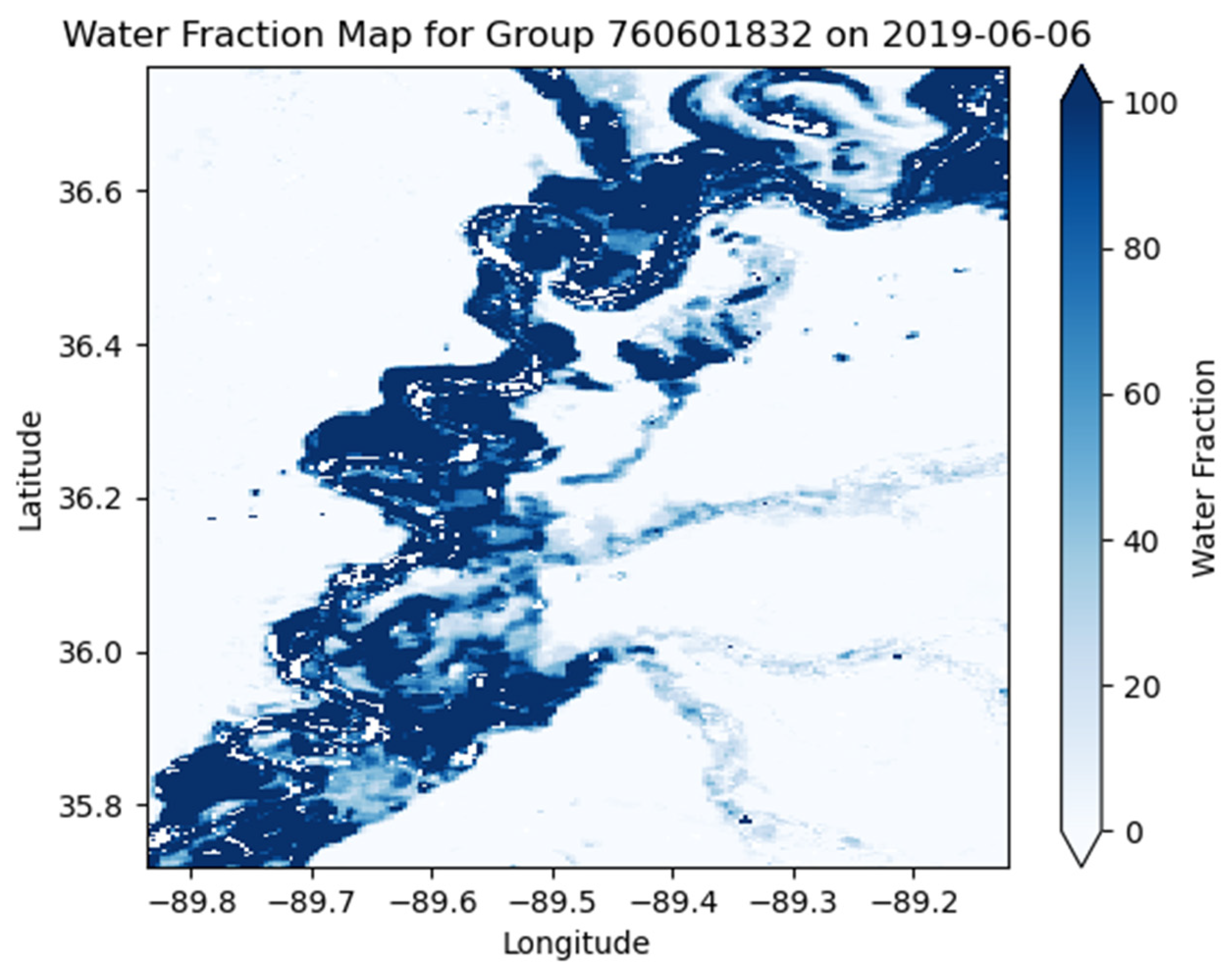
We can see that all the test cases that achieved a performance Category of 5 occurred in areas that have a mean flooding occurrence of over 200. A few of the test cases achieved a Category 4 performance on the catchments with lower means. This shows that even areas with lower flood occurrences might be suitable for model development but are less likely. On some of the lower mean models, NWM provided a better correlation than GEOGLOWS. Because the stream segments are shorter in NWM, it attempts to correlate more reaches per grouped catchment areas; this gives it more chances to find a reach that is significant and not discarded. Conversely, GEOGLOWS arrived at a result for one of the higher mean models where NWM did not. This occurred because GEOGLOWS reports data on every reach, and NWM masks many areas, so data were not available for this area. An example FIER map is shown in
Figure 12.
From the case studies, we can establish a suitability threshold between 150 and 200.
Figure 13 shows all areas that have a mean flood occurrence of 150 or greater. The results show that the Mississippi River and its tributaries are likely suitable. Since FIER models have been created for those areas [
14], we know that they are suitable, and this finding does not contradict our assumption. Many of the catchments along the East Coast and the Gulf of Mexico are shown to be highly suitable. The catchments do not include the ocean, but many of these areas have experienced flooding from hurricanes or tropical storms over the study period. While FIER can be used to model tidal inundation [
13], these areas would likely not be suitable for riverine flood modeling. Many of the areas around the lakes are shown to be highly suitable, but this can include the detection of changes in lake elevation and might not be as suitable as displayed. For this reason, many of the catchment groups north of the Great Lakes that are not masked should be discounted because of the presence of lakes that were too small to be included in our lakes dataset. A similar procedure could be used to evaluate the occurrence of water on the global scale but was not performed in this study because of the required size of the dataset.
4. Discussion
A central finding of the presented research is that the coincidence of flood events and high-quality satellite imagery remains a limiting factor. For SAR-derived synthetic FIM, the primary constraint is spatial and temporal coverage. Many regions are not imaged frequently enough to capture a range of flood magnitudes necessary for robust model development. The suitability classification, based on return periods of observed high flows, reveals that while a significant number of locations are suitable for modeling low-frequency events (e.g., 2-year return periods), only a small fraction—less than 2%—are viable for high-magnitude events such as 50- or 100-year floods. This suggests that while SAR provides high spatial resolution and cloud-penetrating capability, the practical viability of SAR-based FIER models is presently limited to regions with consistent, ongoing satellite tasking and frequent flooding.
Furthermore,
Table 3 shows the theoretical probability of observing a flood of each return period given an increasing number of years. Probabilities are calculated using the exceedance probability formula shown in Equation (1), where P is the probability of a given event occurring in a given year, divided by the return period in years, and n is the number of years of observations. This table does not account for less frequent satellite acquisitions, missed acquisitions due to malfunctioning sensors or clouds blocking an optical sensor, or any of the other limitations discussed in this paper. The calculated probabilities consequently represent the best-case scenarios, and actual probabilities should be much lower after accounting for other mistakes.
Equation (1): Exceedance Probability Formula
Comparing
Table 2, showing the maximum return period observed by image sources considered in this study, and
Table 3, the theoretical best case scenario probabilities, illustrates the limitations induced by infrequent image acquisitions. The satellite sources considered in this paper have all collected data for between 10 and 15 years.
Table 3 suggests the probability of a river having a flood event exceeding the 10-year return period threshold is between 65% and 87%. However,
Table 2 shows that less than 10% of the sampled rivers had such a flood event that was also observed by a satellite image. Waiting for more years of observations should increase the utility of satellite-derived synthetic FIM methods. However, other limitations in the acquisitions, such as decreased coverage and frequency due to the loss of Sentinel 1B and mismatched flood occurrence dates and revisit dates, significantly hamper its utility.
In contrast, the VIIRS-based synthetic FIM suitability analysis, though constrained to North America in this study, reveals broader potential applicability. By processing more than 3500 daily water fraction images and comparing them against a resampled permanent water mask, we derived a mean flood occurrence metric that effectively captures relative suitability for model generation. The VIIRS suitability metric correlates well with FIER model performance: all test cases with a mean flood occurrence exceeding 200 produced high-performing models. However, even locations with lower flood occurrences occasionally yielded viable outputs, indicating some flexibility in the threshold for suitability. Importantly, this suggests that the VIIRS-based process, due to the daily global coverage, is particularly well-suited for large-scale screening of candidate modeling locations.
5. Conclusions
We evaluated viable locations for creating satellite-derived synthetic flood maps. We used FIER as our test model, along with simulated hydrological data from GEOGLOWS and NWM. Simulated hydrological data allow for making models in many ungauged locations. We developed workflows that determine the suitability of an area for satellite-derived synthetic FIM model creation with imagery from VIIRS and SAR based on the coincidence of satellite imagery and flood extents.
We created test case FIER models demonstrating the accuracy of the VIIRS-derived synthetic FIM process and showed which areas were the best for synthetic flood map creation. Our study area for VIIRS was limited to the United States, Canada, and Mexico. Future work could extend the process to be global by processing the rest of the VIIRS images. While we created test cases to determine the feasibility of different areas using VIIRS, we did not examine the accuracy of the models by comparing them to observed extents. There are several general and model-specific items to consider when performing validation on satellite-derived models. Different modeling methods may be variably sensitive or skillful in predicting flood extents outside the range of flows directly observed by satellites. One option that has been previously implemented for FIER model validation is to use the model to predict flooding based on a forecasted flow and then compare the synthetic flood map to the observed satellite imagery once the flood has occurred [
14]. Some modeling methods may not extrapolate outside the range of training flows at all. When satellite observations of higher flows are sparse, suitability may be less than expected based on the presented results. For models of this type, including FIER, the suitability estimates presented represent the upper limits for skillful flood synthesis.
The SAR-derived synthetic FIM feasibility study could be extended to investigate more points, and since the resolution of SAR is much higher, it is possible that flooding could be visible on lower stream order rivers. We did not consider the effects of image correction for geometric or radiometric errors. In areas with steep terrain, this could become a limiting factor. Test cases for SAR models would provide additional insight into the accuracy of our feasibility assessment. The scale of the catchment groups can be adjusted based on the desired model domain or input data. River discharge data that were used to determine which images constituted a flood could easily be replaced with data from another hydrologic model, gauges, or other sources appropriate for the location and other modeling methods.
This study focused on only a single synthetic FIM method, FIER, and the SAR and optical data sources for which it has been developed. However, these methods are adaptable to different sensors or satellites, hydrological inputs, and flood model types. For the VIIRS-derived synthetic FIM process, adjusting what counts as a flooding pixel for model-specific constraints before reducing to a flood occurrence image allows for customization. Other sources of imagery, such as MODIS or Landsat could likewise be categorized and counted.
Optical and SAR data suitability were evaluated individually, and the results highlight the limitation of each in isolation. In the specific case of FIER models, it has been shown that optical and SAR data can be combined [
41]. Further research in satellite-derived FIM synthesis of any methods may need to create or apply methods to incorporate many data sources, potentially including non-satellite acquired datasets. Data fusion techniques to combine SAR and optical data together with other data could also increase the number of areas that are suitable for other synthetic FIM methods in addition to FIER.
The areas shown suitable in this study represent a snapshot based on data that are presently available and not a definitive permanent suitability classification into the future. Suitability is expected to improve at more sites and ranges of flows as more data are collected, additional sensors are included, and data fusion methods are refined. As this occurs, the methods presented in the paper can be reapplied to identify areas that will then become suitable for flood map synthesis.
Author Contributions
Conceptualization, L.P., R.C.H. and E.J.N.; methodology, L.P., R.C.H. and E.J.N.; software, L.P., R.C.H., K.N.M., H.L. and A.R.; validation, L.P., R.C.H., A.R. and H.L.; formal analysis, L.P. and R.C.H.; investigation, L.P.; resources, E.J.N.; data curation, L.P., R.C.H. and K.N.M.; writing—original draft preparation, L.P., R.C.H. and E.J.N.; writing—review and editing, K.N.M., G.P.W., D.P.A., H.L., and A.R.; visualization, L.P. and R.C.H.; supervision, E.J.N., G.P.W. and D.P.A.; project administration, E.J.N. and G.P.W.; funding acquisition, E.J.N. and G.P.W. All authors have read and agreed to the published version of the manuscript.
Funding
Funding for this project was provided by the National Oceanic and Atmospheric Administration (NOAA), awarded to the Cooperative Institute for Research on Hydrology (CIROH) through the NOAA Cooperative Agreement with The University of Alabama, NA22NWS4320003 and under grant number NA20NES4320003 from the NOAA JPSS Program. The statements, findings, conclusions, and recommendations are those of the author(s) and do not necessarily reflect the views of NOAA.
Data Availability Statement
Acknowledgments
We thank Brigham Young University and University of Houston for the many resources provided to facilitate the research presented in this manuscript.
Conflicts of Interest
The authors declare no conflicts of interest. The funders had no role in the design of the study, in the collection, analyses, or interpretation of data, in the writing of the manuscript, or in the decision to publish the results.
Abbreviations
The following abbreviations are used in this manuscript:
| CONUS | Continental United States of America |
| DEM | Digital Elevation Model |
| FFT | Flood Fraction Threshold |
| FIER | Forecasting Inundation Extents using REOF analysis |
| FIM | Flood Inundation Maps |
| GEE | Google Earth Engine |
| JPSS | Joint Polar Satellite System |
| JRC | Joint Research Centre |
| NOAA | National Oceanic and Atmospheric Administration |
| NWM | National Water Model |
| REOF | Rotated Empirical Orthogonal Function |
| SAR | Synthetic Aperture Radar |
| US | United States |
| USGS | United States Geologic Survey |
| VFM | NOAA JPSS/VIIRS Flood Mapping Product |
| VIIRS | Visible Infrared Imaging Radiometer Suite |
Appendix A
Example FIER Outputs from Qualitative Analysis
The following figures are examples of the qualitatively classified maps referenced in
Section 3 and
Section 3.4.
Figure A1 is an example of a spatial mode from a FIER model placed in Category 2 according to
Section 3 and
Section 3.4. The units on the color bar, right, are unitless coefficients of the spatial correlation of that pixel to flooding coming from a principal component analysis. The nearly completely uniform grey color, indicating a coefficient of zero, shows that nearly none of the images has any spatial correlation with flooding.
Figure A1.
Example plot of a FIER spatial mode of a scene placed in Category 2.
Figure A1.
Example plot of a FIER spatial mode of a scene placed in Category 2.
Figure A2 and
Figure A3 show examples of FIER outputs placed in Category 3. The first,
Figure A2, is an example of the lowest flow flood of the month. The second,
Figure A3, is an example of the highest flow flood of the month. The units on the scale bars are in percent water fraction. No change is visible between the two maps, though a significant difference exists between the input flows.
Figure A2.
An example FIER map output placed in Category 3 for the low flow scenario.
Figure A2.
An example FIER map output placed in Category 3 for the low flow scenario.
Figure A3.
An example FIER map output placed in Category 3 for the high flow scenario.
Figure A3.
An example FIER map output placed in Category 3 for the high flow scenario.
Figure A4 and
Figure A5 show examples of FIER outputs placed in Category 3. The first,
Figure A4, is an example of the lowest flow flood of the month. The second,
Figure A5, is an example of the highest flow flood of the month. The units on the scale bars are in percent water fraction. The river is not visible during low flows and becomes barely visible during high flows, but flooding is not observed.
Figure A4.
An example FIER map output placed in Category 4 for the low flow scenario.
Figure A4.
An example FIER map output placed in Category 4 for the low flow scenario.
Figure A5.
An example FIER map output placed in Category 4 for the high flow scenario.
Figure A5.
An example FIER map output placed in Category 4 for the high flow scenario.
Figure A6 and
Figure A7 show examples of FIER outputs placed in Category 3. The first,
Figure A6, is an example of the lowest flow flood of the month. The second,
Figure A7, is an example of the highest flow flood of the month. The units on the scale bars are in percent water fraction. Unlike Category 4, the river is visible in both images, and significant flooding is observed in the high-flow image.
Figure A6.
An example FIER map output placed in Category 5 for the low flow scenario.
Figure A6.
An example FIER map output placed in Category 5 for the low flow scenario.
Figure A7.
An example FIER map output placed in Category 5 for the high flow scenario.
Figure A7.
An example FIER map output placed in Category 5 for the high flow scenario.
Table A1.
Performance of NWM and GEOGLOWS models with different mean flood occurrences from the VIIRS suitability process.
Table A1.
Performance of NWM and GEOGLOWS models with different mean flood occurrences from the VIIRS suitability process.
| Catchment Group | Mean | NWM Results | GEOGLOWS Results |
|---|
| 760593430 | 0 | 1 | 1 |
| 710837546 | 0 | 2 | 1 |
| 760284141 | 10 | 4 | 1 |
| 770169647 | 11 | 2 | 2 |
| 710821624 | 16 | 1 | 1 |
| 720196159 | 18 | 2 | 2 |
| 710423168 | 25 | 2 | 1 |
| 750191337 | 36 | 1 | 1 |
| 720151618 | 59 | 3 | 3 |
| 760291400 | 60 | 4 | 4 |
| 760631679 | 63 | 1 | 1 |
| 760664822 | 79 | 3 | 1 |
| 760686334 | 88 | 1 | 1 |
| 760658166 | 108 | 4 | 4 |
| 720160116 | 126 | 1 | 1 |
| 720148320 | 153 | 2 | 2 |
| 720148320 | 153 | 2 | 2 |
| 760601832 | 216 | 5 | 5 |
| 750230692 | 284 | N/A | 5 |
| 760676450 | 305 | 5 | 5 |
References
- Doocy, S.; Daniels, A.; Murray, S.; Kirsch, T.D. The human impact of floods: A historical review of events 1980–2009 and systematic literature review. PLoS Curr. 2013, 5. [Google Scholar] [CrossRef] [PubMed]
- Moreland, J.A. Floods and Flood Plains; US Geological Survey, US Dept. of the Interior: Washington, DC, USA, 1993.
- Rai, R.K.; van den Homberg, M.J.; Ghimire, G.P.; McQuistan, C. Cost-benefit analysis of flood early warning system in the Karnali River Basin of Nepal. Int. J. Disaster Risk Reduct. 2020, 47, 101534. [Google Scholar] [CrossRef]
- Henao Salgado, M.J.; Zambrano Nájera, J. Assessing flood early warning systems for flash floods. Front. Clim. 2022, 4, 787042. [Google Scholar] [CrossRef]
- Wania, A.; Joubert-Boitat, I.; Dottori, F.; Kalas, M.; Salamon, P. Increasing timeliness of satellite-based flood mapping using early warning systems in the Copernicus Emergency Management Service. Remote Sens. 2021, 13, 2114. [Google Scholar] [CrossRef]
- Bauer-Marschallinger, B.; Cao, S.; Tupas, M.E.; Roth, F.; Navacchi, C.; Melzer, T.; Freeman, V.; Wagner, W. Satellite-Based Flood Mapping through Bayesian Inference from a Sentinel-1 SAR Datacube. Remote Sens. 2022, 14, 3673. [Google Scholar] [CrossRef]
- Coltin, B.; McMichael, S.; Smith, T.; Fong, T. Automatic boosted flood mapping from satellite data. Int. J. Remote Sens. 2016, 37, 993–1015. [Google Scholar] [CrossRef]
- Elkhrachy, I. Flash flood hazard mapping using satellite images and GIS tools: A case study of Najran City, Kingdom of Saudi Arabia (KSA). Egypt. J. Remote Sens. Space Sci. 2015, 18, 261–278. [Google Scholar] [CrossRef]
- Jung, Y.; Kim, D.; Kim, D.; Kim, M.; Lee, S.O. Simplified flood inundation mapping based on flood elevation-discharge rating curves using satellite images in gauged watersheds. Water 2014, 6, 1280–1299. [Google Scholar] [CrossRef]
- Notti, D.; Giordan, D.; Caló, F.; Pepe, A.; Zucca, F.; Galve, J.P. Potential and limitations of open satellite data for flood mapping. Remote Sens. 2018, 10, 1673. [Google Scholar] [CrossRef]
- Revilla-Romero, B.; Hirpa, F.A.; Pozo, J.T.-d.; Salamon, P.; Brakenridge, R.; Pappenberger, F.; De Groeve, T. On the use of global flood forecasts and satellite-derived inundation maps for flood monitoring in data-sparse regions. Remote Sens. 2015, 7, 15702–15728. [Google Scholar] [CrossRef]
- Sjoberg, B.; Li, S.; Sun, D. Global Flood Mapping Services from JPSS. In Proceedings of the IGARSS 2018—2018 IEEE International Geoscience and Remote Sensing Symposium, Valencia, Spain, 22–27 July 2018. [Google Scholar]
- Chang, C.-H.; Lee, H.; Kim, D.; Hwang, E.; Hossain, F.; Chishtie, F.; Jayasinghe, S.; Basnayake, S. Hindcast and forecast of daily inundation extents using satellite SAR and altimetry data with rotated empirical orthogonal function analysis: Case study in Tonle Sap Lake Floodplain. Remote Sens. Environ. 2020, 241, 111732. [Google Scholar] [CrossRef]
- Rostami, A.; Chang, C.-H.; Lee, H.; Wan, H.-H.; Du, T.L.T.; Markert, K.N.; Williams, G.P.; Nelson, E.J.; Li, S.; Straka III, W. Forecasting Flood Inundation in US Flood-Prone Regions Through a Data-Driven Approach (FIER): Using VIIRS Water Fractions and the National Water Model. Remote Sens. 2024, 16, 4357. [Google Scholar] [CrossRef]
- Chang, C.-H.; Lee, H.; Du, L.; Choi, J.; Bui, D.; Meechaiya, C.; Markert, K. Forecasting Inundation Extents using REOF analysis (FIER) over Lower Mekong Basin. In Proceedings of the AGU Fall Meeting Abstracts, Virtual, 1–17 December 2020. [Google Scholar]
- Chang, C.-H.; Lee, H.; Do, S.K.; Du, T.L.; Markert, K.; Hossain, F.; Ahmad, S.K.; Piman, T.; Meechaiya, C.; Bui, D.D. Operational forecasting inundation extents using REOF analysis (FIER) over lower Mekong and its potential economic impact on agriculture. Environ. Model. Softw. 2023, 162, 105643. [Google Scholar] [CrossRef]
- Markert, K.N.; Lee, H.; Williams, G.P.; Nelson, E.J.; Ames, D.P.; Griffin, R.E.; Meyer, F.J. Evaluating the Feasibility of Scaling the FIER Framework for Large-Scale Flood Inundation Prediction. EGUsphere 2024, 2024, 1–34. [Google Scholar]
- Flores-Anderson, A.I.; Herndon, K.E.; Thapa, R.B.; Cherrington, E. The SAR Handbook: Comprehensive Methodologies for Forest Monitoring and Biomass Estimation; SERVIR Global: Washington, DC, USA, 2019. [Google Scholar] [CrossRef]
- Miranda, N.; Torres, R.; Geudtner, D.; Pinheiro, M.; Potin, P.; Gratadour, J.-B.; O’Connell, A.; Bibby, D.; Navas-Traver, I.; Cossu, M. Sentinel-1 First Generation Status, Past and Future. In Proceedings of the IGARSS 2023—2023 IEEE International Geoscience and Remote Sensing Symposium, Pasadena, CA, USA, 16–21 July 2023. [Google Scholar]
- Showstack, R. Sentinel Satellites Initiate New Era in Earth Observation; Wiley Online Library: Hoboken, NJ, USA, 2014. [Google Scholar]
- Torres, R.; Snoeij, P.; Geudtner, D.; Bibby, D.; Davidson, M.; Attema, E.; Potin, P.; Rommen, B.; Floury, N.; Brown, M. GMES Sentinel-1 mission. Remote Sens. Environ. 2012, 120, 9–24. [Google Scholar] [CrossRef]
- Copernicus. Overview of Sentinel-1. 2024. Available online: https://sentiwiki.copernicus.eu/web/s1-mission (accessed on 26 September 2024).
- Ager, T.P. An introduction to synthetic aperture radar imaging. Oceanography 2013, 26, 20–33. [Google Scholar] [CrossRef]
- Dekker, R.J. Speckle filtering in satellite SAR change detection imagery. Int. J. Remote Sens. 1998, 19, 1133–1146. [Google Scholar] [CrossRef]
- Domg, Y.; Milne, A.K. Toward edge sharpening: A SAR speckle filtering algorithm. IEEE Trans. Geosci. Remote Sens. 2001, 39, 851–863. [Google Scholar] [CrossRef]
- Martinis, S.; Plank, S.; Ćwik, K. The use of Sentinel-1 time-series data to improve flood monitoring in arid areas. Remote Sens. 2018, 10, 583. [Google Scholar] [CrossRef]
- Li, S.; Sun, D.; Goldberg, M.D.; Sjoberg, B.; Santek, D.; Hoffman, J.P.; DeWeese, M.; Restrepo, P.; Lindsey, S.; Holloway, E. Automatic near real-time flood detection using Suomi-NPP/VIIRS data. Remote Sens. Environ. 2018, 204, 672–689. [Google Scholar] [CrossRef]
- Li, S.; Sun, D. JPSS VIIRS Flood Mapping (VFM) Algorithm Theoretical Basis Document. 2021. Available online: https://www.ssec.wisc.edu/flood-map-demo/wp-content/uploads/sites/38/2021/06/ATBD-JPSS_VFM_V1.1_June23_2021.pdf (accessed on 1 January 2025).
- Cao, C.; Blonski, S.; Wang, W.; Uprety, S.; Shao, X.; Choi, J.; Lynch, E.; Kalluri, S. NOAA-20 VIIRS on-orbit performance, data quality, and operational Cal/Val support. In Proceedings of the Earth Observing Missions and Sensors: Development, Implementation, and Characterization V, Honolulu, HI, USA, 25–26 September 2018. [Google Scholar]
- Huang, C.; Chen, Y.; Wu, J.; Li, L.; Liu, R. An evaluation of Suomi NPP-VIIRS data for surface water detection. Remote Sens. Lett. 2015, 6, 155–164. [Google Scholar] [CrossRef]
- Xiong, X.; Angal, A.; Sun, J.; Lei, N.; Twedt, K.; Chen, H.; Chiang, K. An overview of NOAA-21 VIIRS early on-orbit calibration and performance. Sens. Syst. Next-Gener. Satell. XXVII 2023, 12729, 308–317. [Google Scholar]
- Ekeu-Wei, I.T. Evaluation of hydrological data collection challenges and flood estimation uncertainties in Nigeria. Environ. Nat. Resour. Res. 2018, 8, 44–54. [Google Scholar] [CrossRef]
- Kumar, V.; Sen, S. Rating curve development and uncertainty analysis in mountainous watersheds for informed hydrology and resource management. Front. Water 2024, 5, 1323139. [Google Scholar] [CrossRef]
- Krabbenhoft, C.A.; Allen, G.H.; Lin, P.; Godsey, S.E.; Allen, D.C.; Burrows, R.M.; DelVecchia, A.G.; Fritz, K.M.; Shanafield, M.; Burgin, A.J.; et al. Assessing placement bias of the global river gauge network. Nat. Sustain. 2022, 5, 586–592. [Google Scholar] [CrossRef]
- Hales, R.C.; Nelson, E.J.; Souffront, M.; Gutierrez, A.L.; Prudhomme, C.; Kopp, S.; Ames, D.P.; Williams, G.P.; Jones, N.L. Advancing global hydrologic modeling with the GEOGloWS ECMWF streamflow service. J. Flood Risk Manag. 2022, 18, e12859. [Google Scholar] [CrossRef]
- Cosgrove, B.; Gochis, D.; Flowers, T.; Dugger, A.; Ogden, F.; Graziano, T.; Clark, E.; Cabell, R.; Casiday, N.; Cui, Z. NOAA’s National Water Model: Advancing operational hydrology through continental-scale modeling. JAWRA J. Am. Water Resour. Assoc. 2024, 60, 247–272. [Google Scholar] [CrossRef]
- Strahler, A.N. Quantitative analysis of watershed geomorphology. Eos Trans. Am. Geophys. Union 1957, 38, 913–920. [Google Scholar]
- Carlson, K.A.; Levin, H.K.; Morris, A.L.; Candela, S.G.; Rivera, A.M.M.; Huening, V.G.; Fredericks, J.G. TDX-Hydro: Global High-Resolution Hydrography Derived from TanDEM-X. Authorea Prepr. 2024. [Google Scholar]
- Lehner, B.; Anand, M.; Fluet-Chouinard, E.; Tan, F.; Aires, F.; Allen, G.H.; Bousquet, P.; Canadell, J.G.; Davidson, N.; Finlayson, C.M. Mapping the world’s inland surface waters: An update to the Global Lakes and Wetlands Database (GLWD v2). Earth Syst. Sci. Data Discuss. 2024, 2024, 1–49. [Google Scholar]
- Scheidegger, A. Effect of map scale on stream orders. Hydrol. Sci. J. 1966, 11, 56–61. [Google Scholar] [CrossRef]
- Markert, K.N.; Williams, G.P.; Nelson, E.J.; Ames, D.P.; Lee, H.; Griffin, R.E. Dense Time Series Generation of Surface Water Extents through Optical–SAR Sensor Fusion and Gap Filling. Remote Sens. 2024, 16, 1262. [Google Scholar] [CrossRef]
| Disclaimer/Publisher’s Note: The statements, opinions and data contained in all publications are solely those of the individual author(s) and contributor(s) and not of MDPI and/or the editor(s). MDPI and/or the editor(s) disclaim responsibility for any injury to people or property resulting from any ideas, methods, instructions or products referred to in the content. |
© 2025 by the authors. Licensee MDPI, Basel, Switzerland. This article is an open access article distributed under the terms and conditions of the Creative Commons Attribution (CC BY) license (https://creativecommons.org/licenses/by/4.0/).

 ,
, 


