


Influences of Sampling Design and Model Selection on Predictions of Chemical Compounds in Petroferric Formations in the Brazilian Amazon

 , , , , , and
Abstract
1. Introduction
2. Materials and Methods
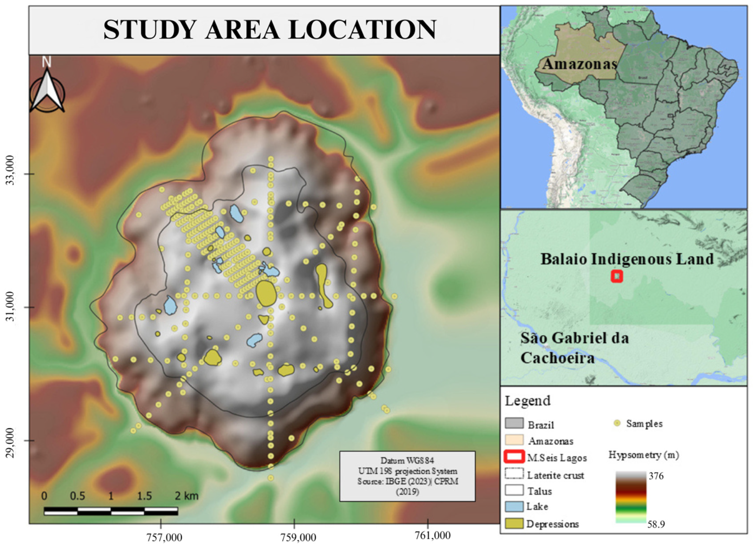
2.1. Study Area
2.2. Environmental Covariates
2.3. Selection of Environmental Covariates
2.4. Modelling
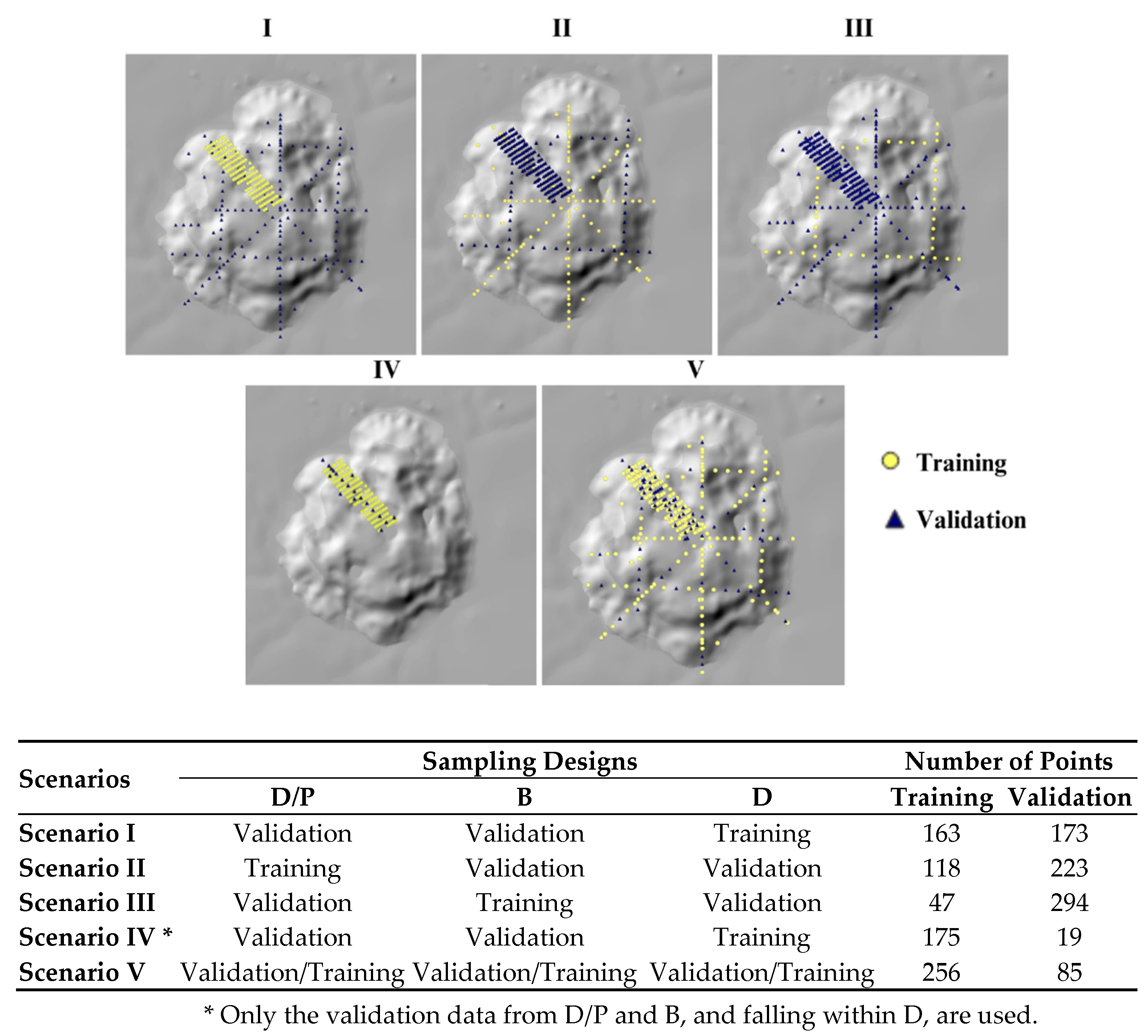
2.5. Sampling Scenarios
2.6. Model Performance Evaluation
3. Results
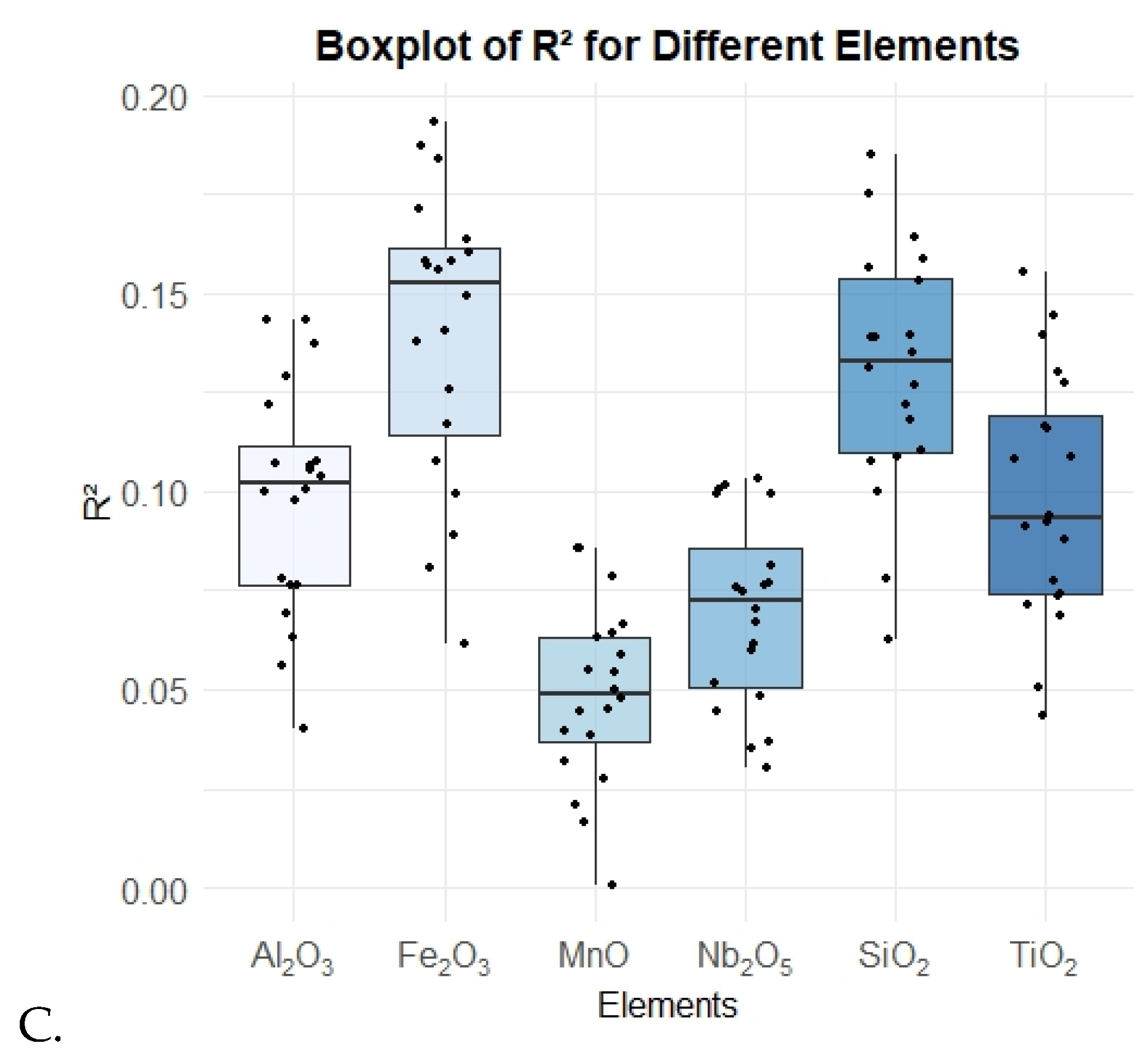
3.1. Factors Influencing Performance
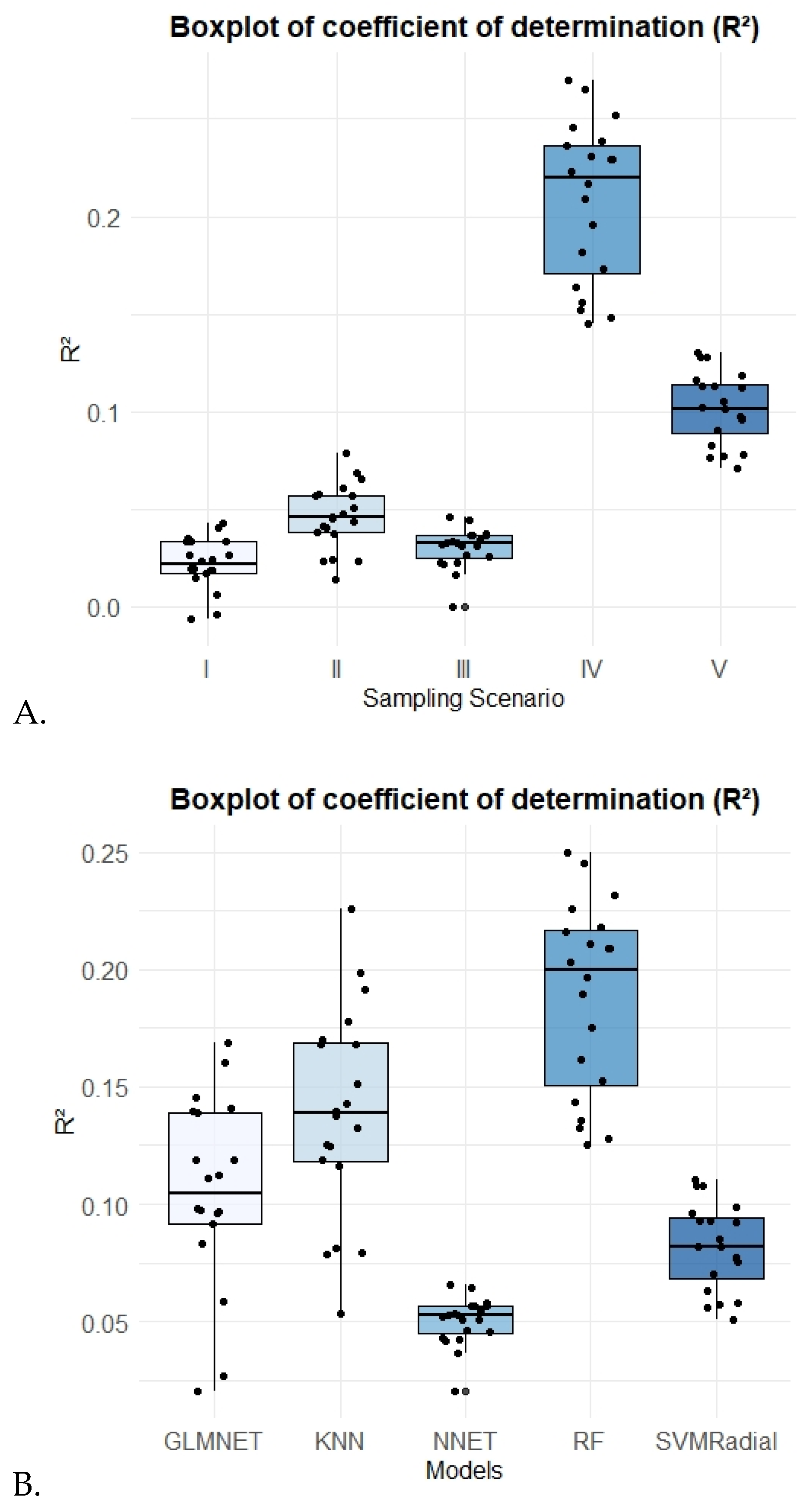
3.2. Accuracy Prediction Comparisons Among Scenarios
3.3. Accuracy Predictions Among Models
3.4. Interaction of Models and Sampling Scenarios in Accuracy Predictions
4. Discussion
4.1. Influence of Sampling Scenarios
4.2. Spatial Variability and Geological Context
4.3. Geological Formation of the Study Area
4.4. Predictive Models
4.5. Sampling Designs and Properties
5. Conclusions
Supplementary Materials
Author Contributions
Funding
Data Availability Statement
Conflicts of Interest
References
- Jenny, H. Factors of Soil Formation: A System of Quantitative Pedology; McGraw-Hill Book Co.: New York, NY, USA, 1941. [Google Scholar]
- McBratney, A.B.; Mendonça Santos, M.L.; Minasny, B. On Digital Soil Mapping. Geoderma 2003, 117, 3–52. [Google Scholar] [CrossRef]
- Runge, E.C.A. Soil Development Sequences and Energy Models. Soil Sci. 1973, 115, 183–193. [Google Scholar] [CrossRef]
- Simonson, R.W. A Multiple-Process Model of Soil Genesis. In Quaternary Soils; Geo Abstracts: Norwich, UK, 1978; pp. 1–25. ISBN 0-86094-012-8. [Google Scholar]
- Kämpf, N.; Curi, N. Formacao e Evolucao Do Solo (Pedogênese). In Pedologia: Fundamentos, SBCS (School of Business and Computer Science); Ker, J.C., Curi, N., Schaefer, C.E.G.R., Vidal-Torrado, P., Eds.; Brazilian Society of Soil Science: Viçosa, Brazil, 2012; pp. 207–302. [Google Scholar]
- Pinheiro Junior, C.R.; Pereira, M.G.; Silva Neto, E.C.; Anjos, L.H.C. Soils of Brazil: Genesis, Classification and Limitations to Use. In Soils of Brazil; Atena: Ponta Grossa, Brazil, 2020; pp. 183–199. [Google Scholar]
- Giovannini, A.L.; Mitchell, R.H.; Neto, A.C.B.; Moura, C.A.V.; Pereira, V.P.; Porto, C.G. Mineralogy and Geochemistry of the Morro Dos Seis Lagos Siderite Carbonatite, Amazonas, Brazil. Lithos 2020, 360–361, 105433. [Google Scholar] [CrossRef]
- Zardiackas, L.D.; Kraay, M.J.; Freese, H.L.; International, A. Titanium, Niobium, Zirconium, and Tantalum for Medical and Surgical Applications; ASTM STP 1471; ASTM: West Conshohocken, PA, USA, 2006; ISBN 978-0-8031-3497-3. [Google Scholar]
- Babaei, K.; Fattah-alhosseini, A.; Chaharmahali, R. A Review on Plasma Electrolytic Oxidation (PEO) of Niobium: Mechanism, Properties and Applications. Surf. Interfaces 2020, 21, 100719. [Google Scholar] [CrossRef]
- Chen, Q.; Thouas, G.A. Metallic Implant Biomaterials. Mater. Sci. Eng. R Rep. 2015, 87, 1–57. [Google Scholar] [CrossRef]
- Giovannini, A.L.; Neto, A.C.B.; Porto, C.G.; Takehara, L.; Pereira, V.P.; Bidone, M.H. REE Mineralization (Primary, Supergene and Sedimentary) Associated to the Morro Dos Seis Lagos Nb (REE, Ti) Deposit (Amazonas, Brazil). Ore Geol. Rev. 2021, 137, 104308. [Google Scholar] [CrossRef]
- Palmieri, M.; Brod, J.A.; Cordeiro, P.; Gaspar, J.C.; Barbosa, P.A.R.; de Assis, L.C.; Junqueira-Brod, T.C.; e Silva, S.E.; Milanezi, B.P.; Machado, S.A.; et al. The Carbonatite-Related Morro Do Padre Niobium Deposit, Catalão II Complex, Central Brazil. Econ. Geol. 2022, 117, 1497–1520. [Google Scholar] [CrossRef]
- Giovannini, A.L.; Neto, A.C.B.; Porto, C.G.; Pereira, V.P.; Takehara, L.; Barbanson, L.; Bastos, P.H.S. Mineralogy and Geochemistry of Laterites from the Morro Dos Seis Lagos Nb (Ti, REE) Deposit (Amazonas, Brazil). Ore Geol. Rev. 2017, 88, 461–480. [Google Scholar] [CrossRef]
- Ferreira, A.C.S.; Pinheiro, É.F.M.; Costa, E.M.; Ceddia, M.B. Predicting Soil Carbon Stock in Remote Areas of the Central Amazon Region Using Machine Learning Techniques. Geoderma Reg. 2023, 32, e00614. [Google Scholar] [CrossRef]
- Gelsleichter, Y.A.; Costa, E.M.; dos Anjos, L.H.C.; Marcondes, R.A.T. Enhancing Soil Mapping with Hyperspectral Subsurface Images Generated from Soil Lab Vis-SWIR Spectra Tested in Southern Brazil. Geoderma Reg. 2023, 33, e00641. [Google Scholar] [CrossRef]
- Padarian, J.; Minasny, B.; McBratney, A.B. Machine Learning and Soil Sciences: A Review Aided by Machine Learning Tools. Soil 2020, 6, 35–52. [Google Scholar] [CrossRef]
- Wadoux, A.M.J.-C.; Brus, D.J.; Heuvelink, G.B.M. Sampling Design Optimization for Soil Mapping with Random Forest. Geoderma 2019, 355, 113913. [Google Scholar] [CrossRef]
- Minasny, B.; McBratney, A.B. A Conditioned Latin Hypercube Method for Sampling in the Presence of Ancillary Information. Comput. Geosci. 2006, 32, 1378–1388. [Google Scholar] [CrossRef]
- Roudier, P. Clhs: A R Package for Conditioned Latin Hypercube Sampling; R Foundation for Statistical Computing: Vienna, Austria, 2011. [Google Scholar]
- de Viegas Filho, J.R.; Bonow, C.W. Seis Lagos Project: Final Report; CPRM: Manaus, Brazil, 1976. [Google Scholar]
- Justo, L.J.E.C. Projeto Uaupés: Relatório Final de Pesquisa; CPRM: Manaus, Brazil, 1983. [Google Scholar]
- Takehara, L.; Almeida, M. Informe de Recursos Minerais—Avaliação do Potencial de Terras Raras no Brasil—Área Seis Lagos, Estado do Amazonas; Serviço Geológico do Brasil—CPRM: Brasília, Brazil, 2019. [Google Scholar]
- Hengl, T.; Nussbaum, M.; Wright, M.N.; Heuvelink, G.B.M.; Gräler, B. Random Forest as a Generic Framework for Predictive Modeling of Spatial and Spatio-Temporal Variables. PeerJ 2018, 6, e5518. [Google Scholar] [CrossRef]
- Friedman, J.; Hastie, T.; Tibshirani, R. Regularization Paths for Generalized Linear Models via Coordinate Descent. J. Stat. Softw. 2010, 33, 1–22. [Google Scholar] [CrossRef]
- Venables, W.N.; Ripley, B.D. Modern Applied Statistics with S, 4th ed.; Springer: New York, NY, USA, 2002. [Google Scholar]
- Hechenbichler, K.; Schliep, K. Weighted K-Nearest-Neighbor Techniques and Ordinal Classification; LMU Munich: Munich, Germany, 2004; discussion paper 399. [Google Scholar]
- Breiman, L. Random Forests. Mach. Learn. 2001, 45, 5–32. [Google Scholar] [CrossRef]
- McRoberts, R.E. Estimating Forest Attribute Parameters for Small Areas Using Nearest Neighbors Techniques. For. Ecol. Manag. 2012, 272, 3–12. [Google Scholar] [CrossRef]
- Heung, B.; Bulmer, C.E.; Schmidt, M.G. Predictive Soil Parent Material Mapping at a Regional-Scale: A Random Forest Approach. Geoderma 2014, 214–215, 141–154. [Google Scholar] [CrossRef]
- Dias, R.L.S.; da Silva, D.D.; Fernandes-Filho, E.I.; do Amaral, C.H.; dos Santos, E.P.; Marques, J.F.; Veloso, G.V. Machine Learning Models Applied to TSS Estimation in a Reservoir Using Multispectral Sensor Onboard to RPA. Ecol. Inform. 2021, 65, 101414. [Google Scholar] [CrossRef]
- Duan, M.; Song, X.; Li, Z.; Zhang, X.; Ding, X.; Cui, D. Identifying Soil Groups and Selecting a High-Accuracy Classification Method Based on Multi-Textural Features with Optimal Window Sizes Using Remote Sensing Images. Ecol. Inform. 2024, 81, 102563. [Google Scholar] [CrossRef]
- BRASIL Decree Law No. 9.985, of 18 July 2000. Establishes the National System of Nature Conservation Units (SNUC). Available online: https://www.planalto.gov.br/ccivil_03/decreto/2000/D9985.htm (accessed on 26 April 2025).
- R Core Team. R: A Language and Environment for Statistical Computing; R Foundation for Statistical Computing: Vienna, Austria, 2021. [Google Scholar]
- RStudio Team. RStudio: Integrated Development Environment for R; RStudio, PBC: Boston, MA, USA, 2020. [Google Scholar]
- ESRI. ArcGIS Desktop, version 10.6; ESRI: Redlands, CA, USA, 2016. [Google Scholar]
- Conrad, O.; Bechtel, B.; Bock, M.; Dietrich, H.; Fischer, E.; Gerlitz, L.; Wehberg, J.; Wichmann, V.; Böhner, J. System for Automated Geoscientific Analyses (SAGA) v. 2.1.4. Geosci. Model Dev. 2015, 8, 1991–2007. [Google Scholar] [CrossRef]
- IBGE – Instituto Brasileiro de Geografia e Estatística. Modelos Digitais de Superfície – MDS. Available online: https://www.ibge.gov.br/geociencias/informacoes-ambientais/modelo-digital-de-terreno/15851-modelos-digitais-de-superficie.html (accessed on 26 April 2025).
- Sora, A.M.; Simbe, M.; Dias, J.; Uacane, M.S. Integration of Satellite Images to Identify Changes in the Xiluvo-Nhamatanda Carbonatite Suite. Educ.-Educ. Soc. Environ. 2018, 21, 251–263. Available online: https://periodicos.ufam.edu.br/index.php/educamazonia/article/view/5106 (accessed on 26 April 2025).
- Jeong, G.; Oeverdieck, H.; Park, S.J.; Huwe, B.; Ließ, M. Spatial Soil Nutrients Prediction Using Three Supervised Learning Methods for Assessment of Land Potentials in Complex Terrain. Catena 2017, 154, 73–84. [Google Scholar] [CrossRef]
- Svetnik, V.; Liaw, A.; Tong, C.; Wang, T. Application of Breiman’s Random Forest to Modeling Structure-Activity Relationships of Pharmaceutical Molecules. In Multiple Classifier Systems; Roli, F., Kittler, J., Windeatt, T., Eds.; Springer: Berlin/Heidelberg, Germany, 2004; pp. 334–343. [Google Scholar]
- Kuhn, M. Building Predictive Models in R Using the Caret Package. J. Stat. Softw. 2008, 28, 1–26. [Google Scholar] [CrossRef]
- Silveira, C.T.; Oka-Fiori, C.; Santos, L.J.C.; Sirtoli, A.E.; Silva, C.R.; Botelho, M.F. Soil Prediction Using Artificial Neural Networks and Topographic Attributes. Geoderma 2013, 195–196, 165–172. [Google Scholar] [CrossRef]
- Liaw, A.; Wiener, M. Classification and Regression by randomForest. R News 2002, 2, 18–22. [Google Scholar]
- Karatzoglou, A.; Smola, A.; Hornik, K. Kernlab: Kernel-Based Machine Learning Lab; CRAN: Vienna, Austria, 2024. [Google Scholar]
- Reis, G.B.; da Silva, D.D.; Filho, E.I.F.; Moreira, M.C.; Veloso, G.V.; de Fraga, M.S.; Pinheiro, S.A.R. Effect of Environmental Covariable Selection in the Hydrological Modeling Using Machine Learning Models to Predict Daily Streamflow. J. Environ. Manag. 2021, 290, 112625. [Google Scholar] [CrossRef]
- Moquedace, C.M.; Baldi, C.G.O.; Siqueira, R.G.; Cardoso, I.M.; de Souza, E.F.M.; Fontes, R.L.F.; Francelino, M.R.; Gomes, L.C.; Fernandes-Filho, E.I. High-Resolution Mapping of Soil Carbon Stocks in the Western Amazon. Geoderma Reg. 2024, 36, e00773. [Google Scholar] [CrossRef]
- Ditzler, C.; Scheffe, K.; Monger, H.C. (Eds.) Soil Survey Staff Soil Survey Manual; USDA Handbook: Washington, DC, USA, 2017. [Google Scholar]
- Rodrigues, H.M.; Vasques, G.M.; Oliveira, R.P.; Tavares, S.R.L.; Ceddia, M.B.; Hernani, L.C. Finding Suitable Transect Spacing and Sampling Designs for Accurate Soil ECa Mapping from EM38-MK2. Soil Syst. 2020, 4, 56. [Google Scholar] [CrossRef]
- Grimm, R.; Behrens, T.; Märker, M.; Elsenbeer, H. Soil Organic Carbon Concentrations and Stocks on Barro Colorado Island—Digital Soil Mapping Using Random Forests Analysis. Geoderma 2008, 146, 102–113. [Google Scholar] [CrossRef]
- Kirkwood, C.; Cave, M.; Beamish, D.; Grebby, S.; Ferreira, A. A Machine Learning Approach to Geochemical Mapping. J. Geochem. Explor. 2016, 167, 49–61. [Google Scholar] [CrossRef]
- Bento, J.P.P.; Porto, C.G.; Takehara, L.; da Silva, F.J.; Bastos Neto, A.C.; Machado, M.L.; Duarte, A.C. Mineral Potential Re-Evaluation of the Seis Lagos Carbonatite Complex, Amazon, Brazil. Braz. J. Geol. 2022, 52, e20210031. [Google Scholar] [CrossRef]
- Odeh, I.O.A.; McBratney, A.B.; Chittleborough, D.J. Further Results on Prediction of Soil Properties from Terrain Attributes: Heterotopic Cokriging and Regression-Kriging. Geoderma 1995, 67, 215–226. [Google Scholar] [CrossRef]
- McKenzie, N.J.; Ryan, P.J. Spatial Prediction of Soil Properties Using Environmental Correlation. Geoderma 1999, 89, 67–94. [Google Scholar] [CrossRef]
- Stumpf, F.; Schmidt, K.; Behrens, T.; Schönbrodt-Stitt, S.; Buzzo, G.; Dumperth, C.; Wadoux, A.; Xiang, W.; Scholten, T. Incorporating Limited Field Operability and Legacy Soil Samples in a Hypercube Sampling Design for Digital Soil Mapping. J. Plant Nutr. Soil Sci. 2016, 179, 499–509. [Google Scholar] [CrossRef]
- Muhindo, K.G. Geology, Geochemistry and Economic Potential of the Bingo Carbonatite and Its Associated Laterites in Beni Territory, North Kivu, Democratic Republic of Congo (DRC). Master’s Thesis, University of Nairobi, Nairobi, Kenya, 2018. [Google Scholar]
- de Oliveira, J.R.S.; Pruski, F.F.; da Silva, J.M.A.; da Silva, D.P. Comparative Analysis of the Performance of Mixed Terraces and Level and Graded Terraces. Acta Sci. Agron. 2012, 34, 351–357. [Google Scholar] [CrossRef]
- Rodrigues, N.; Lopes da Silva, J.C.; Pereira Marinatti da Silva, R.; Saraiva Koenow Pinheiro, H.; Carvalho Junior, W. Mapping of Fe2O3, Nb and TiO2, as a Support to Classify Outcropping Materials in “Morro DOS Seis Lagos” Carbonatite Complex, Brazilian Amazon. In Proceedings of the EGU General Assembly, Vienna, Austria, 23–27 May 2022; EGU22-12326. [Google Scholar]
- Guimarães, J.T.F.; Sahoo, P.K.; e Souza-Filho, P.W.M.; da Silva, M.S.; Rodrigues, T.M.; da Silva, E.F.; Reis, L.S.; de Figueiredo, M.M.J.C.; da Lopes, K.S.; Moraes, A.M.; et al. Landscape and Climate Changes in Southeastern Amazonia from Quaternary Records of Upland Lakes. Atmosphere 2023, 14, 621. [Google Scholar] [CrossRef]
- Safaee, S.; Libohova, Z.; Kladivko, E.J.; Brown, A.; Winzeler, E.; Read, Q.; Rahmani, S.; Adhikari, K. Influence of Sample Size, Model Selection, and Land Use on Prediction Accuracy of Soil Properties. Geoderma Reg. 2024, 36, e00766. [Google Scholar] [CrossRef]
- Malone, B.P.; Minasny, B.; Odgers, N.P.; McBratney, A.B. Using Model Averaging to Combine Soil Property Rasters from Legacy Soil Maps and from Point Data. Geoderma 2014, 232–234, 34–44. [Google Scholar] [CrossRef]
- Zhang, J.; Schmidt, M.G.; Heung, B.; Bulmer, C.E.; Knudby, A. Using an Ensemble Learning Approach in Digital Soil Mapping of Soil pH for the Thompson-Okanagan Region of British Columbia. Can. J. Soil Sci. 2022, 102, 579–596. [Google Scholar] [CrossRef]
- De Oliveira, S.M.B.; Pessenda, L.C.R.; Gouveia, S.E.M.; Fávaro, D.I.T.; Babinski, M. Geochemical Evidence of Soils Formed by the Interaction of Guano with Volcanic Rocks, Rata Island, Fernando de Noronha (PE). Geologia USP. Sci. Ser. 2009, 9, 3–12. [Google Scholar]
- Matschullat, J.; Martins, G.C.; Enzweiler, J.; von Fromm, S.F.; van Leeuwen, J.; de Lima, R.M.B.; Schneider, M.; Zurba, K. What Influences Upland Soil Chemistry in the Amazon Basin, Brazil? Major, Minor and Trace Elements in the Upper Rhizosphere. J. Geochem. Explor. 2020, 211, 106433. [Google Scholar] [CrossRef]
- Thompson, J.A.; Bell, J.C.; Butler, C.A. Digital elevation model resolution: Effects on terrain attribute calculation and quantitative soil-landscape modeling. Geoderma 2001, 100, 67–89. [Google Scholar] [CrossRef]
- Wilson, J.P.; Gallant, J.C.; Walsh, S.J. Topographic Mapping and Analysis in GIS. In Geographic Information Systems and Science; Ramsay, R.H., McCleary, R.E., Eds.; IntechOpen: London, UK, 2007; pp. 87–112. [Google Scholar]
- Hutchinson, M.F.; Gallant, J.C. Digital elevation models and representation of terrain shape. Math. Comput. Simul. 2000, 42, 135–150. [Google Scholar]
- Moore, I.D.; Burch, G.J. Physical basis of the length-slope factor in the Universal Soil Loss Equation. Soil Sci. Soc. Am. J. 1986, 50, 1294–1298. [Google Scholar] [CrossRef]
- Olaya, V. SAGA GIS—Morphometry Tools. 2004. Available online: https://saga-gis.sourceforge.io/saga_tool_doc/2.2.3/ta_morphometry_6.html (accessed on 26 April 2025).
- Conrad, O. Mid-Slope Position Analysis in SAGA GIS; Geoscientific Model Development; SAGA GIS: San Diego, CA, USA, 2008. [Google Scholar]
- Gallant, J.C.; Dowling, T.I. A multiresolution index of valley bottom flatness for mapping depositional areas. Water Resour. Res. 2003, 39, 12. [Google Scholar] [CrossRef]
- Conrad, O. Slope Index Calculation in SAGA GIS; SAGA GIS Documentation; SAGA GIS: San Diego, CA, USA, 2010. [Google Scholar]
- Rouse, J.W.; Haas, R.H.; Schell, J.A.; Deering, D.W. Monitoring vegetation systems in the Great Plains with ERTS. NASA Spec. Publ. 1973, 351, 309–317. [Google Scholar]
- Huete, A.R. A soil-adjusted vegetation index (SAVI). Remote Sens. Environ. 1988, 25, 295–309. [Google Scholar] [CrossRef]
- Van der Meer, F.D.; Van der Werff, H.M.A.; Van Ruitenbeek, F.J.A.; Hecker, C.A.; Bakker, W.H.; Noomen, M.F.; Woldai, T. Multi-and hyperspectral geologic remote sensing: A review. Int. J. Appl. Earth Obs. Geoinf. 2014, 33, 161–175. [Google Scholar] [CrossRef]
- Sabins, F.F. Remote Sensing Principles and Interpretation, 3rd ed.; W.H. Freeman and Company: New York, NY, USA, 1997. [Google Scholar]
- Kalinowski, A.; Oliver, S. ASTER Mineral Index Processing Manual; Geoscience Australia Technical Report; Geoscience Australia: Canberra, Australia, 2004. [Google Scholar]
- Rowan, L.C.; Mars, J.C.; Simpson, C.J. Hyperspectral analysis of the ultramafic complex of the Gossan Lead, Virginia, USA. Remote Sens. Environ. 2003, 88, 123–139. [Google Scholar]
- Sora, S.; Van der Meer, F.; Hecker, C. Spectral indices for detecting advanced argillic alteration in active hydrothermal systems. Int. J. Appl. Earth Obs. Geoinf. 2018, 69, 134–147. [Google Scholar]
- European Space Agency (ESA). Sentinel-1 SAR User Guide; ESA: Paris, France, 2021; Available online: https://sentinel.esa.int (accessed on 10 January 2024).


| Elements (% Wt) | Geology | Mean | Median | Min. | Max. | SD | CV (%) | Cs | Ck |
|---|---|---|---|---|---|---|---|---|---|
| Al2O3 | Combined | 3.28 | 1.67 | 0.19 | 58.0 | 6.4 | 195.9 | 5.3 | 31.4 |
| Laterite/Depressions | 4.73 | 1.76 | 0.75 | 36.7 | 8.9 | 189.4 | 3.0 | 7.8 | |
| Laterite | 2.07 | 1.42 | 0.19 | 32.5 | 3.1 | 148.2 | 7.4 | 65.4 | |
| Talus | 6.31 | 2.71 | 0.26 | 58.0 | 10.5 | 165.6 | 3.1 | 9.6 | |
| Fe2O3 | Combined | 67.0 | 77.4 | 0.12 | 95.1 | 22.6 | 508.0 | 1.7 | 1.9 |
| Laterite/Depressions | 68.6 | 73.9 | 7.10 | 87.5 | 19.7 | 28.7 | 19.7 | 3.5 | |
| Laterite | 75.8 | 78.8 | 6.96 | 95.1 | 13.5 | 17.9 | −2.1 | 6.3 | |
| Talus | 51.3 | 61.0 | 0.12 | 92.7 | 31 | 60.3 | −0.4 | −1.5 | |
| TiO2 | Combined | 2.93 | 1.42 | bdl | 29.9 | 4.1 | 16.7 | 2.8 | 9.9 |
| Laterite/Depressions | 4.82 | 2.36 | 0.73 | 17.1 | 4.9 | 100.9 | 1.3 | 0.3 | |
| Laterite | 3.46 | 1.86 | 0.04 | 29.9 | 4.4 | 126.6 | 2.5 | 8.2 | |
| Talus | 1.25 | 0.50 | bdl | 18.3 | 2.3 | 182.1 | 5.0 | 33.1 | |
| Nb2O5 | Combined | 0.74 | 0.39 | 0.00 | 4.02 | 0.9 | 0.8 | 1.4 | 1.5 |
| Laterite/Depressions | 1.53 | 1.12 | 0.53 | 3.81 | 1.0 | 66.9 | 0.9 | −0.4 | |
| Laterite | 0.81 | 0.49 | bdl | 4.02 | 0.9 | 111.8 | 1.2 | 0.8 | |
| Talus | 0.34 | 0.22 | bdl | 2.38 | 0.5 | 149.0 | 2.2 | 4.8 | |
| MnO | Combined | 5.09 | 0.20 | bdl | 64.1 | 14.0 | 2.8 | 10.9 | 3.0 |
| Laterite/Depressions | 0.41 | 0.06 | bdl | 4.51 | 1.1 | 272.6 | 3.1 | 8.1 | |
| Laterite | 1.62 | 0.17 | bdl | 63.8 | 6.8 | 416.5 | 6.5 | 47.0 | |
| Talus | 14.67 | 0.66 | bdl | 64.1 | 22.0 | 150.1 | 1.1 | −0.4 | |
| SiO2 | Combined | 2.74 | 0.56 | bdl | 97.8 | 11.6 | 422.6 | 7.0 | 50.7 |
| Laterite/Depressions | 2.95 | 0.56 | 0.12 | 36.5 | 9.3 | 314.3 | 3.1 | 8.5 | |
| Laterite | 0.84 | 0.46 | bdl | 26.7 | 2.2 | 259.7 | 9.3 | 95.9 | |
| Talus | 7.86 | 1.45 | 0.14 | 97.8 | 21.5 | 273.7 | 3.5 | 10.9 |
| RMSE | |||||
| Source of Variation | DF | SS | MS | F | p-Value |
| Scenario | 4 | 551.2 | 137.8 | 1.7 | 0.15 |
| Model | 4 | 1415.5 | 353.9 | 4.0 | 0.00 |
| Element | 5 | 16,731.6 | 3346.3 | 41.5 | 0.00 |
| Scenario x Model | 16 | 58.4 | 3.7 | 0.04 | 1.00 |
| Error | 120 | 9675.9 | 80.6 | ||
| MAE | |||||
| Source of Variation | DF | SS | MS | F | p-Value |
| Scenaio | 4 | 127.7 | 31.9 | 0.4 | 0.79 |
| Model | 4 | 1404.7 | 351.2 | 4.6 | 0.00 |
| Element | 5 | 11,783.7 | 2356.7 | 30.6 | 0.00 |
| Scenario x Model | 16 | 48.1 | 3.0 | 0.03 | 1.00 |
| Error | 120 | 9247.0 | 77.1 | ||
| R2 | |||||
| Source of Variation | DF | SS | MS | F | p-Value |
| SCENARIO | 4 | 1.0 | 0.25 | 41.22 | 0.00 |
| Model | 4 | 0.1 | 0.02 | 4.5 | 0.00 |
| Element | 5 | 0.1 | 0.02 | 3.6 | 0.00 |
| Scenario x Model | 16 | 0.2 | 0 | 1.6 | 0.08 |
| Error | 120 | 0.8 | 0 | ||
| Model | Training | Validation | ||||
|---|---|---|---|---|---|---|
| RMSE | MAE | R2 | RMSE | MAE | R2 | |
| NNET | 17.05 a | 13.47 a | 0.08 d | 18.52 a | 13.58 a | 0.05 b |
| SVMRadial | 7.87 b | 4.15 b | 0.56 b | 10.44 b | 5.19 b | 0.04 b |
| GLMNET | 7.51 b | 4.8 b | 0.93 a | 11.06 b | 6.62 b | 0.08 ab |
| KNN | 7.36 b | 4.36 b | 0.16 cd | 11.12 b | 6.14 b | 0.11 a |
| RF | 7.16 b | 4.27 b | 0.22 c | 10.84 b | 6.16 b | 0.1 ab |
| Element | RMSE | MAE | R2 | RMSE | MAE | R2 |
| Fe2O3 | 29.17 a | 24.23 a | 0.34 a | 32.64 a | 26.69 a | 0.14 a |
| MnO | 11.81 b | 5.44 b | 0.47 a | 15.36 b | 7.96 b | 0.06 b |
| SiO2 | 6.07 bc | 2.43 b | 0.34 a | 15.4 b | 4.72 bc | 0.06 b |
| Al2O3 | 5.07 bc | 2.43 b | 0.4 a | 5.65 c | 2.51 bc | 0.06 b |
| TiO2 | 3.4 c | 2.13 b | 0.36 a | 4.52 c | 2.7 bc | 0.07 b |
| Nb2O5 | 0.81 c | 0.61 b | 0.42 a | 0.81 c | 0.64 c | 0.07 b |
| Training | Validation | ||||||||
|---|---|---|---|---|---|---|---|---|---|
| Element (%) | Scenario | RMSE | MAE | R2 | RMSE | MAE | R2 | Pc | Bias |
| Al2O3 | I | 1.99 | 1.20 | 0.33 | 9.08 | 3.54 | 0.02 | 0.11 | −2.33 |
| II | 9.58 | 4.56 | 0.46 | 4.22 | 2.49 | 0.02 | 0.07 | 0.24 | |
| III | 6.63 | 3.04 | 0.48 | 6.57 | 2.79 | 0.01 | 0.04 | −0.35 | |
| IV | 2.02 | 1.22 | 0.31 | 1.59 | 1.21 | 0.24 | 0.32 | −0.02 | |
| V | 6.63 | 2.84 | 0.43 | 6.02 | 2.47 | 0.04 | 0.15 | −0.25 | |
| Mean | 5.37 | 2.57 | 0.40 | 5.50 | 2.50 | 0.07 | 0.14 | −0.54 | |
| Fe2O3 | I | 27.82 | 23.27 | 0.44 | 35.80 | 29.72 | 0.09 | 0.24 | 16.85 |
| II | 33.92 | 27.19 | 0.23 | 30.79 | 26.12 | 0.07 | 0.22 | 15.87 | |
| III | 25.21 | 22.17 | 0.39 | 34.20 | 26.86 | 0.02 | 0.95 | −9.96 | |
| IV | 28.50 | 23.74 | 0.39 | 32.40 | 25.46 | 0.44 | 0.53 | −4.39 | |
| V | 30.43 | 24.84 | 0.30 | 30.01 | 25.33 | 0.09 | 0.25 | 17.29 | |
| Mean | 29.18 | 24.24 | 0.35 | 32.64 | 26.70 | 0.14 | 0.44 | 12.87 | |
| MnO | I | 12.13 | 5.84 | 0.50 | 18.21 | 11.71 | 0.03 | 0.16 | 6.52 |
| II | 13.64 | 5.87 | 0.42 | 13.51 | 6.17 | 0.12 | 0.27 | −2.18 | |
| III | 7.03 | 3.19 | 0.32 | 15.00 | 6.31 | 0.02 | 0.11 | −3.38 | |
| IV | 12.73 | 5.90 | 0.58 | 21.09 | 11.46 | 0.13 | 0.32 | −2.46 | |
| V | 13.51 | 6.38 | 0.59 | 9.05 | 4.24 | 0.03 | −0.21 | 1.88 | |
| Mean | 11.81 | 5.44 | 0.48 | 15.37 | 7.98 | 0.07 | 0.13 | 0.07 | |
| Nb2O5 | I | 0.86 | 0.65 | 0.34 | 0.89 | 0.63 | 0.02 | 0.06 | −0.12 |
| II | 0.70 | 0.54 | 0.47 | 0.91 | 0.72 | 0.03 | 0.16 | 0.05 | |
| III | 0.84 | 0.59 | 0.38 | 0.96 | 0.77 | 0.02 | 0.02 | 0.10 | |
| IV | 0.86 | 0.66 | 0.47 | 0.46 | 0.38 | 0.26 | 0.29 | −0.01 | |
| V | 0.83 | 0.62 | 0.49 | 0.87 | 0.71 | 0.07 | 0.25 | 0.09 | |
| Mean | 0.82 | 0.61 | 0.43 | 0.82 | 0.64 | 0.08 | 0.16 | 0.02 | |
| TiO2 | I | 4.59 | 2.81 | 0.32 | 3.76 | 2.69 | 0.03 | 0.13 | 0.07 |
| II | 3.28 | 2.05 | 0.28 | 4.57 | 2.69 | 0.05 | 0.20 | −0.95 | |
| III | 2.60 | 1.73 | 0.30 | 4.61 | 2.66 | 0.01 | −0.26 | −0.88 | |
| IV | 4.49 | 2.73 | 0.31 | 4.72 | 2.94 | 0.21 | 0.43 | −1.48 | |
| V | 4.04 | 2.45 | 0.46 | 4.12 | 2.54 | 0.08 | 0.25 | −0.66 | |
| Mean | 3.80 | 2.36 | 0.33 | 4.36 | 2.71 | 0.07 | 0.15 | −0.78 | |
| SiO2 | I | 3.64 | 2.26 | 0.34 | 4.47 | 2.71 | 0.08 | 0.15 | −0.95 |
| II | 16.30 | 7.39 | 0.27 | 4.59 | 2.80 | 0.05 | 0.68 | 1.82 | |
| III | 2.33 | 1.21 | 0.29 | 12.61 | 3.12 | 0.01 | 0.01 | −1.44 | |
| IV | 0.70 | 0.38 | 0.36 | 28.79 | 9.51 | 0.20 | 0.39 | −9.26 | |
| V | 10.21 | 2.77 | 0.51 | 14.26 | 3.65 | 0.00 | 0.04 | −0.98 | |
| Mean | 6.64 | 2.80 | 0.35 | 12.94 | 4.36 | 0.07 | 0.25 | −2.16 | |
| Element (%) | Model | RMSE | MAE | R2 | RMSE | MAE | R2 | Pc | Bias |
|---|---|---|---|---|---|---|---|---|---|
| Training | Validation | ||||||||
| Al2O3 | RF | 5.16 | 2.62 | 0.12 | 5.51 | 2.64 | 0.06 | 0.19 | 0.20 |
| SVMRadial | 5.30 | 2.21 | 0.64 | 5.30 | 2.05 | 0.09 | 0.17 | −1.03 | |
| NNET | 5.82 | 2.46 | 0.17 | 5.69 | 2.24 | 0.05 | −0.10 | −2.06 | |
| GLMNET | 5.27 | 2.77 | 1.00 | 5.38 | 2.77 | 0.09 | 0.26 | −0.10 | |
| KNN | 5.29 | 2.80 | 0.08 | 5.58 | 2.80 | 0.08 | 0.24 | 0.22 | |
| Mean | 5.37 | 2.57 | 0.40 | 5.50 | 2.50 | 0.07 | 0.15 | −0.56 | |
| Fe2O3 | RF | 17.36 | 12.47 | 0.34 | 22.37 | 16.57 | 0.18 | −1.54 | 0.35 |
| SVMRadial | 19.16 | 13.06 | 0.39 | 22.82 | 15.51 | 0.11 | 4.22 | 0.26 | |
| NNET | 71.85 | 68.53 | 0.04 | 70.78 | 66.61 | 0.05 | −66.58 | 0.01 | |
| GLMNET | 18.42 | 13.63 | 0.76 | 24.41 | 18.26 | 0.17 | 1.00 | 0.31 | |
| KNN | 19.08 | 13.50 | 0.21 | 22.83 | 16.53 | 0.20 | −0.57 | 0.40 | |
| Mean | 29.18 | 24.24 | 0.35 | 32.64 | 26.70 | 0.14 | −12.69 | 0.27 | |
| MnO | RF | 10.65 | 5.25 | 0.31 | 14.47 | 7.55 | 0.08 | 1.21 | 0.14 |
| SVMRadial | 12.48 | 4.98 | 0.78 | 14.37 | 6.18 | 0.02 | −3.08 | 0.09 | |
| NNET | 13.82 | 5.11 | 0.04 | 14.29 | 5.36 | 0.06 | −4.44 | 0.13 | |
| GLMNET | 11.11 | 6.58 | 1.00 | 15.59 | 9.78 | 0.09 | 1.88 | 0.29 | |
| KNN | 11.37 | 5.48 | 0.26 | 16.15 | 8.83 | 0.08 | 1.96 | 0.22 | |
| Mean | 11.88 | 5.48 | 0.48 | 14.97 | 7.54 | 0.07 | −0.50 | 0.18 | |
| Nb2O5 | RF | 0.38 | 0.70 | 0.47 | 0.44 | 0.75 | 0.37 | 0.18 | 0.08 |
| SVMRadial | 0.70 | 0.80 | 0.68 | 0.22 | 0.78 | 0.61 | −0.01 | −0.03 | |
| NNET | 0.26 | 0.78 | 0.50 | 0.22 | 0.78 | 0.50 | 0.10 | −0.01 | |
| GLMNET | 0.97 | 1.29 | 1.00 | 0.21 | 1.50 | 0.93 | 0.11 | −0.10 | |
| KNN | 0.27 | 0.78 | 0.51 | 0.34 | 0.77 | 0.51 | 0.33 | 0.07 | |
| Mean | 0.52 | 0.87 | 0.64 | 0.28 | 0.92 | 0.59 | 0.14 | 0.00 | |
| TiO2 | RF | 3.48 | 2.28 | 0.19 | 4.19 | 2.72 | 0.12 | 0.25 | −0.11 |
| SVMRadial | 3.80 | 2.32 | 0.32 | 4.38 | 2.63 | 0.02 | 0.07 | −1.01 | |
| NNET | 4.33 | 2.34 | 0.04 | 4.66 | 2.52 | 0.04 | 0.18 | −2.12 | |
| GLMNET | 3.20 | 2.55 | 1.00 | 3.88 | 3.33 | 0.51 | −0.03 | −0.62 | |
| KNN | 3.74 | 2.40 | 0.12 | 4.08 | 2.61 | 0.12 | 0.22 | −0.17 | |
| Mean | 3.71 | 2.38 | 0.37 | 4.24 | 2.76 | 0.16 | 0.14 | −0.81 | |
| SiO2 | RF | 6.11 | 2.69 | 0.19 | 15.73 | 4.82 | 0.07 | 0.69 | −2.95 |
| SVMRadial | 6.06 | 1.97 | 0.35 | 14.68 | 4.10 | 0.03 | 0.11 | −3.58 | |
| NNET | 6.15 | 2.04 | 0.13 | 14.67 | 4.06 | 0.08 | 0.18 | −3.55 | |
| GLMNET | 6.15 | 3.00 | 0.86 | 15.72 | 5.37 | 0.09 | 0.23 | −1.94 | |
| KNN | 5.77 | 2.42 | 0.22 | 16.28 | 5.26 | 0.06 | 0.17 | −2.13 | |
| Mean | 6.05 | 2.43 | 0.35 | 15.41 | 4.72 | 0.07 | 0.27 | −2.83 | |
Disclaimer/Publisher’s Note: The statements, opinions and data contained in all publications are solely those of the individual author(s) and contributor(s) and not of MDPI and/or the editor(s). MDPI and/or the editor(s) disclaim responsibility for any injury to people or property resulting from any ideas, methods, instructions or products referred to in the content. |
© 2025 by the authors. Licensee MDPI, Basel, Switzerland. This article is an open access article distributed under the terms and conditions of the Creative Commons Attribution (CC BY) license (https://creativecommons.org/licenses/by/4.0/).
Share and Cite
Rodrigues, N.B.; Barbosa, T.R.; Pinheiro, H.S.K.; Mancini, M.; Read, Q.D.; Blackstock, J.; Winzeler, E.H.; Miller, D.; Owens, P.R.; Libohova, Z. Influences of Sampling Design and Model Selection on Predictions of Chemical Compounds in Petroferric Formations in the Brazilian Amazon. Remote Sens. 2025, 17, 1644. https://doi.org/10.3390/rs17091644
Rodrigues NB, Barbosa TR, Pinheiro HSK, Mancini M, Read QD, Blackstock J, Winzeler EH, Miller D, Owens PR, Libohova Z. Influences of Sampling Design and Model Selection on Predictions of Chemical Compounds in Petroferric Formations in the Brazilian Amazon. Remote Sensing. 2025; 17(9):1644. https://doi.org/10.3390/rs17091644
Chicago/Turabian StyleRodrigues, Niriele Bruno, Theresa Rocco Barbosa, Helena Saraiva Koenow Pinheiro, Marcelo Mancini, Quentin D. Read, Joshua Blackstock, Edwin H. Winzeler, David Miller, Phillip R. Owens, and Zamir Libohova. 2025. "Influences of Sampling Design and Model Selection on Predictions of Chemical Compounds in Petroferric Formations in the Brazilian Amazon" Remote Sensing 17, no. 9: 1644. https://doi.org/10.3390/rs17091644
APA StyleRodrigues, N. B., Barbosa, T. R., Pinheiro, H. S. K., Mancini, M., Read, Q. D., Blackstock, J., Winzeler, E. H., Miller, D., Owens, P. R., & Libohova, Z. (2025). Influences of Sampling Design and Model Selection on Predictions of Chemical Compounds in Petroferric Formations in the Brazilian Amazon. Remote Sensing, 17(9), 1644. https://doi.org/10.3390/rs17091644