


Unveiling the Effects of Crop Rotation on Cropland Soil pH Mapping: A Remote Sensing-Based Soil Sample Grouping Strategy
 ,
,  , ,
, , 
Abstract
1. Introduction
2. Materials and Methods
2.1. Study Region
2.2. Data Collection
2.2.1. Soil Samples
2.2.2. Environmental Variables
2.2.3. Crop Rotation
2.2.4. Sentinel Images
2.2.5. Other Variables
2.3. Soil pH Mapping Framework
2.3.1. Variable Scenario and Variable Selection
2.3.2. Modeling for Each Scenario
2.3.3. Grouping by Cropland and Crop Rotation
2.3.4. Model Validation
3. Results
3.1. Modeling for Each Scenario
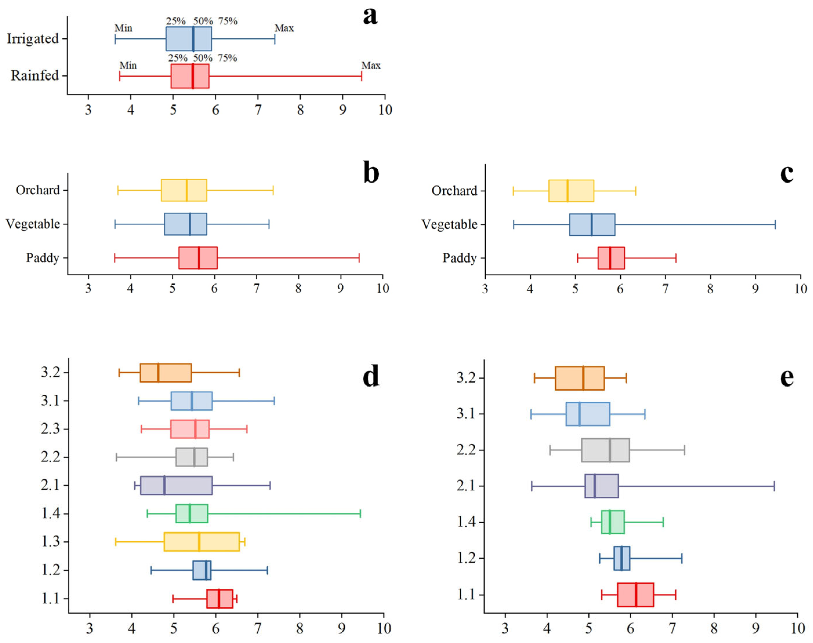
3.2. Grouping by Cropland and Crop Rotation
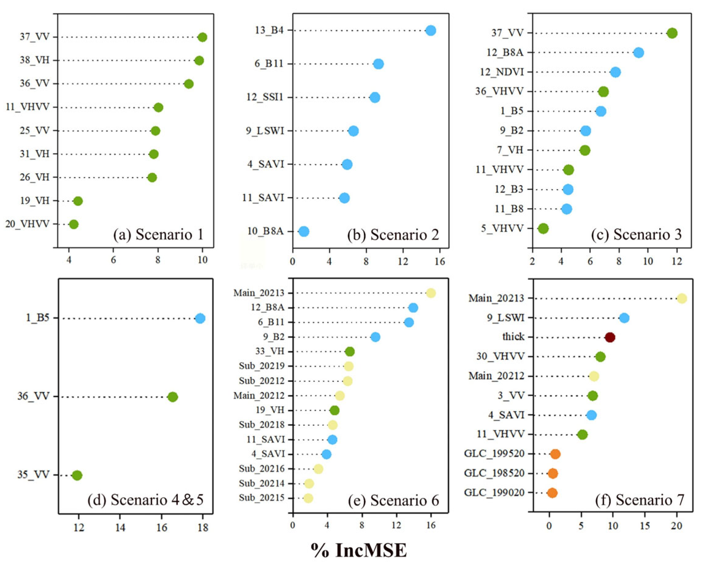
3.3. Relative Variable Importance
3.3.1. Modeling for Each Scenario
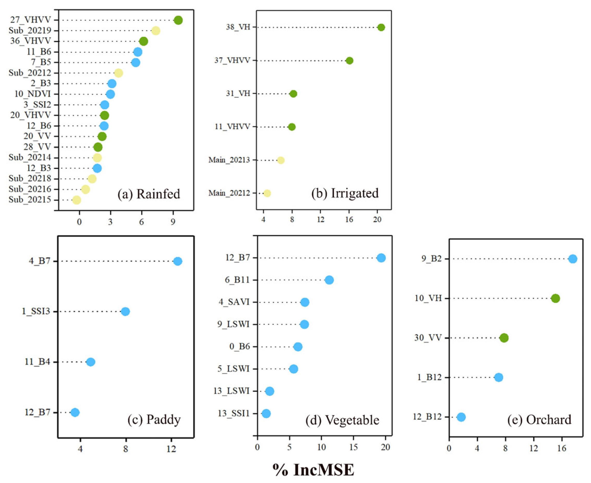
3.3.2. Grouping by Cropland and Crop Rotation
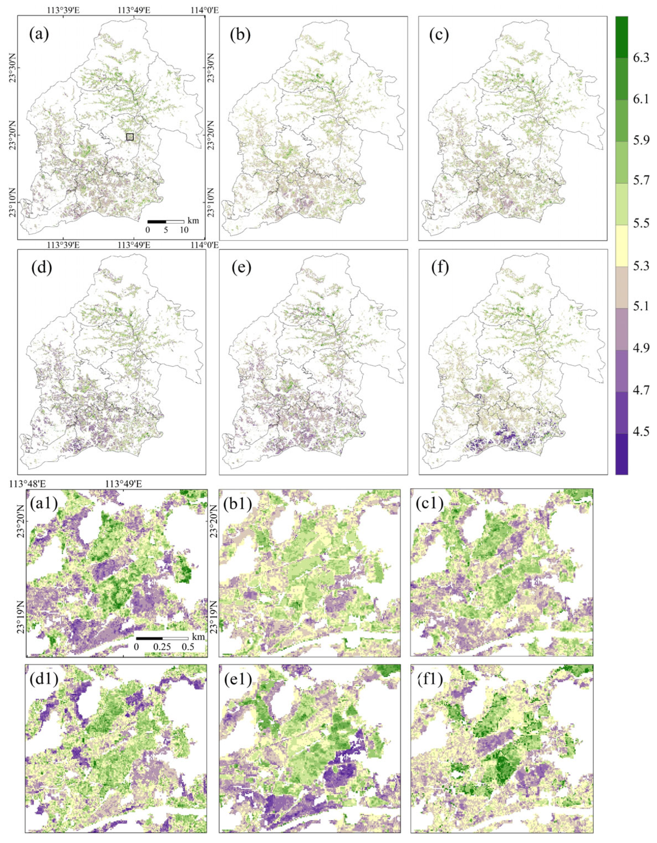
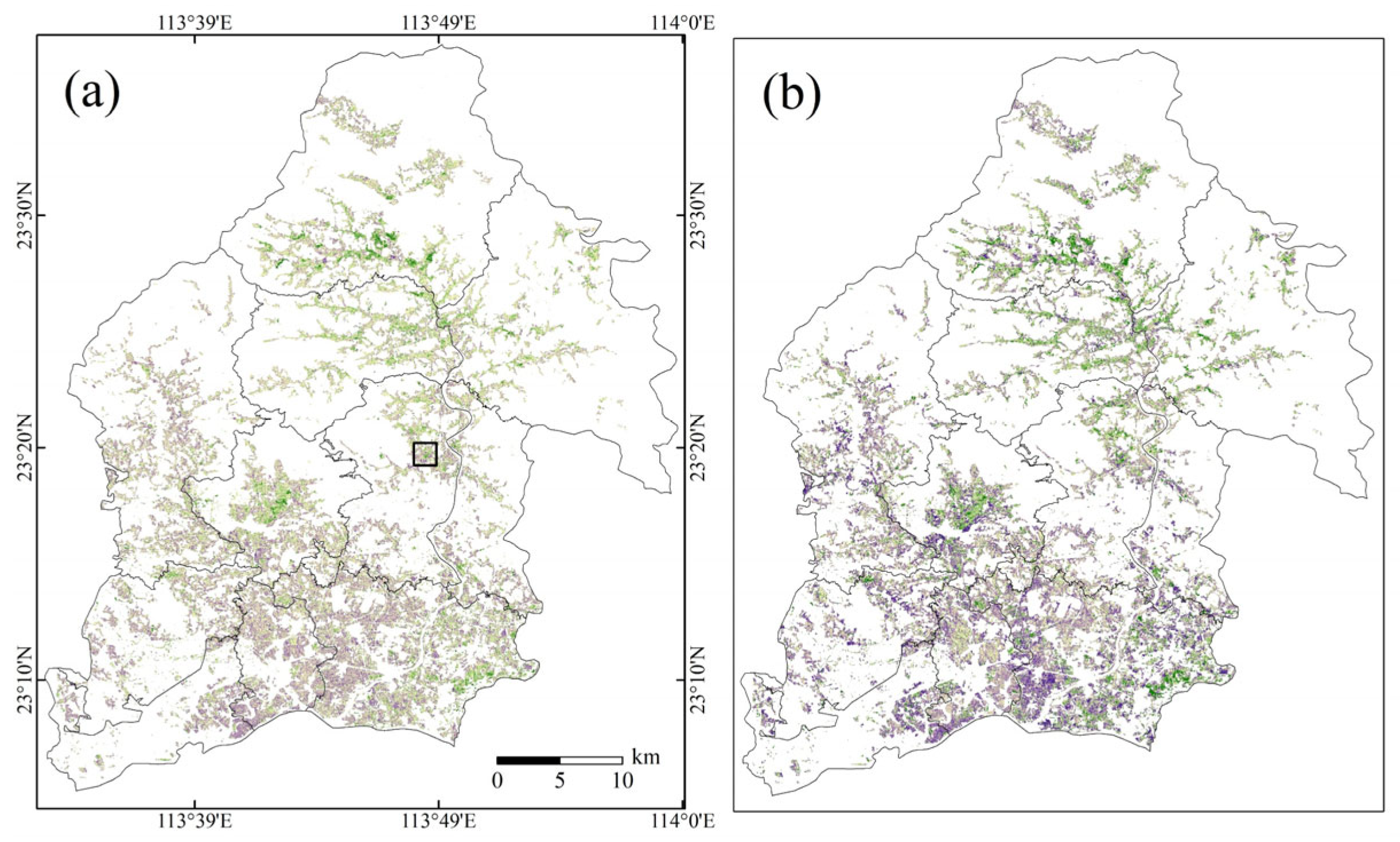
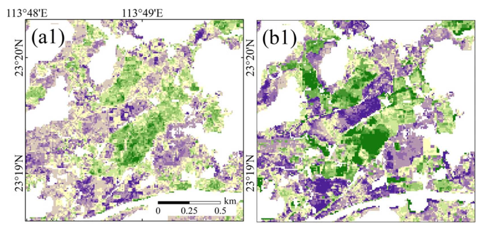
3.4. Spatial Distribution of Soil pH
4. Discussion
4.1. Modeling for Each Scenario
4.2. Grouping by Cropland and Crop Rotation
4.3. Limitations
4.4. Implications
5. Conclusions
Author Contributions
Funding
Data Availability Statement
Conflicts of Interest
Abbreviations
| DSM | Digital soil mapping |
| RMSE | Root mean squared error |
| N | Nitrogen |
| GLC_FCS30 | Global land-cover product with fine classification system at 30 m |
| GPS | Global positioning system |
| Scorpan-SSPFe | Soil spatial prediction function with spatially autocorrelated errors and reference |
| VH | Vertical–horizontal |
| VV | Vertical–vertical |
| CR | Cross-polarization ratio |
| NDVI | Normalized difference vegetation index |
| SAVI | Soil-adjusted vegetation index |
| LSWI | Land surface water index |
| SSI1 | Soil salinity index 1 |
| SSI2 | Soil salinity index 2 |
| SSI3 | Soil salinity index 3 |
| SOC | Soil organic carbon |
| SOM | Soil organic matter |
| MAT | Mean annual temperature |
| MAP | Mean annual precipitation |
| LST | Land surface temperature |
| TWI | Topographic wetness index |
| PLC | Plan curvature |
| PRC | Profile curvature |
| LS | Slope-length factor |
| VD | Valley depth |
| CI | Convergence index |
| CNBL | Channel network base level |
| RSP | Relative slope position |
| CND | Catchment network distance |
| VDCN | Vertical distance to channel network |
| RF | Random forest |
| MSI | Multispectral imager |
| SAR | Synthetic aperture radar |
| GRD | Ground range-detected |
| GEE | Google Earth Engine |
| NSIGC | High-resolution National Soil Information Grids of China |
| SRTM | Shuttle Radar Topographic Mission |
| RFE | Recursive feature elimination |
| MGFS | Modified greedy feature selection |
| mtry | Number of variables randomly sampled as candidates at each split |
| ntree | Number of trees |
| ME | Mean error |
| R2 | Coefficient of determination |
| %IncMSE | Increase in mean square error |
References
- Neina, D. The Role of Soil PH in Plant Nutrition and Soil Remediation. Appl. Environ. Soil Sci. 2019, 2019, 1–9. [Google Scholar] [CrossRef]
- Tan, K.; Wang, H.; Chen, L.; Du, Q.; Du, P.; Pan, C. Estimation of the Spatial Distribution of Heavy Metal in Agricultural Soils Using Airborne Hyperspectral Imaging and Random Forest. J. Hazard. Mater. 2020, 382, 120987. [Google Scholar] [CrossRef] [PubMed]
- Xu, D.; Shen, Z.; Dou, C.; Dou, Z.; Li, Y.; Gao, Y.; Sun, Q. Effects of Soil Properties on Heavy Metal Bioavailability and Accumulation in Crop Grains under Different Farmland Use Patterns. Sci. Rep. 2022, 12, 9211. [Google Scholar] [CrossRef] [PubMed]
- Breemen, V.N.; Mulder, J.; Driscoll, C.T. Acidification and Alkalinization of Soils. Plant Soil 1983, 75, 283–308. [Google Scholar] [CrossRef]
- Breemen, V.N.; Driscoll, C.T.; Mulder, J. Acidic Deposition and Internal Proton Sources in Acidification of Soils and Waters. Nature 1984, 307, 599–604. [Google Scholar] [CrossRef]
- von Uexküll, H.R.; Mutert, E. Global Extent, Development and Economic Impact of Acid Soils. Plant Soil 1995, 171, 1–15. [Google Scholar] [CrossRef]
- Naz, M.; Dai, Z.; Hussain, S.; Tariq, M.; Danish, S.; Khan, I.U.; Qi, S.; Du, D. The Soil PH and Heavy Metals Revealed Their Impact on Soil Microbial Community. J. Environ. Manage. 2022, 321, 115770. [Google Scholar] [CrossRef] [PubMed]
- Zhu, X.F.; Shen, R.F. Towards Sustainable Use of Acidic Soils: Deciphering Aluminum-Resistant Mechanisms in Plants. Fundam. Res. 2023, 4, 1533–1541. [Google Scholar] [CrossRef]
- Kochian, L.V.; Piñeros, M.A.; Liu, J.; Magalhaes, J.V. Plant Adaptation to Acid Soils: The Molecular Basis for Crop Aluminum Resistance. Annu. Rev. Plant Biol. 2015, 66, 571–598. [Google Scholar] [CrossRef]
- Guo, J.H.; Liu, X.J.; Zhang, Y.; Shen, J.L.; Han, W.X.; Zhang, W.F.; Christie, P.; Goulding, K.W.T.; Vitousek, P.M.; Zhang, F.S. Significant Acidification in Major Chinese Croplands. Science 2010, 327, 1008–1010. [Google Scholar] [CrossRef]
- Lu, X.; Zhang, X.; Zhan, N.; Wang, Z.; Li, S. Factors Contributing to Soil Acidification in the Past Two Decades in China. Environ. Earth Sci. 2023, 82, 74. [Google Scholar] [CrossRef]
- Zhu, Q.; Liu, X.; Hao, T.; Zeng, M.; Shen, J.; Zhang, F.; de Vries, W. Cropland Acidification Increases Risk of Yield Losses and Food Insecurity in China. Environ. Pollut. 2020, 256, 113145. [Google Scholar] [CrossRef]
- McBratney, A.B.; Mendonça Santos, M.L.; Minasny, B. On Digital Soil Mapping. Geoderma 2003, 117, 3–52. [Google Scholar] [CrossRef]
- Minasny, B.; McBratney, A.B. Digital Soil Mapping: A Brief History and Some Lessons. Geoderma 2016, 264, 301–311. [Google Scholar] [CrossRef]
- Sünnemann, M.; Beugnon, R.; Breitkreuz, C.; Buscot, F.; Cesarz, S.; Jones, A.; Lehmann, A.; Lochner, A.; Orgiazzi, A.; Reitz, T.; et al. Climate Change and Cropland Management Compromise Soil Integrity and Multifunctionality. Commun. Earth Environ. 2023, 4, 394. [Google Scholar] [CrossRef]
- Meng, H.; Xu, M.; Lv, J.; He, X.H.; Wang, B.; Cai, Z. Quantification of Anthropogenic Acidification under Long-Term Fertilization in the Upland Red Soil of South China. Soil Sci. 2014, 179, 486–494. [Google Scholar] [CrossRef]
- Shin, J.; Won, J.; Kim, S.M.; Kim, D.C.; Cho, Y. Fertilization Mapping Based on the Soil Properties of Paddy Fields in Korea. Agric. 2023, 13, 2049. [Google Scholar] [CrossRef]
- Adalibieke, W.; Cui, X.; Cai, H.; You, L.; Zhou, F. Global Crop-Specific Nitrogen Fertilization Dataset in 1961–2020. Sci. Data 2023, 10, 617. [Google Scholar] [CrossRef] [PubMed]
- Wang, X.; Dou, Z.; Shi, X.; Zou, C.; Liu, D.; Wang, Z.; Guan, X.; Sun, Y.; Wu, G.; Zhang, B.; et al. Innovative Management Programme Reduces Environmental Impacts in Chinese Vegetable Production. Nat. Food 2021, 2, 47–53. [Google Scholar] [CrossRef]
- Zhao, J.; Liu, Z.; Zhai, B.; Jin, H.; Xu, X.; Zhu, Y. Long-Term Changes in Soil Chemical Properties with Cropland-to-Orchard Conversion on the Loess Plateau, China: Regulatory Factors and Relations with Apple Yield. Agric. Syst. 2023, 204, 103562. [Google Scholar] [CrossRef]
- Lu, H.-L.; Li, K.-W.; Nkoh, J.N.; He, X.; Xu, R.-K.; Qian, W.; Shi, R.-Y.; Hong, Z.-N. Effects of PH Variations Caused by Redox Reactions and PH Buffering Capacity on Cd(II) Speciation in Paddy Soils during Submerging/Draining Alternation. Ecotoxicol. Environ. Saf. 2022, 234, 113409. [Google Scholar] [CrossRef] [PubMed]
- Li, B.; Zhu, D.; Li, J.; Liu, X.; Yan, B.; Mao, L.; Zhang, M.; Wang, Y.; Li, X. Converting Upland to Paddy Fields Alters Soil Nitrogen Microbial Functions at Different Depths in Black Soil Region. Agric. Ecosyst. Environ. 2024, 372, 109089. [Google Scholar] [CrossRef]
- Wu, Z.; Sun, X.; Sun, Y.; Yan, J.; Zhao, Y.; Chen, J. Soil Acidification and Factors Controlling Topsoil PH Shift of Cropland in Central China from 2008 to 2018. Geoderma 2022, 408, 115586. [Google Scholar] [CrossRef]
- Hao, T.; Liu, X.; Zhu, Q.; Zeng, M.; Chen, X.; Yang, L.; Shen, J.; Shi, X.; Zhang, F.; de Vries, W. Quantifying Drivers of Soil Acidification in Three Chinese Cropping Systems. Soil Tillage Res. 2022, 215, 105230. [Google Scholar] [CrossRef]
- Waldhoff, G.; Lussem, U.; Bareth, G. Multi-Data Approach for Remote Sensing-Based Regional Crop Rotation Mapping: A Case Study for the Rur Catchment, Germany. Int. J. Appl. Earth Obs. Geoinf. 2017, 61, 55–69. [Google Scholar] [CrossRef]
- Li, R.; Xu, M.; Chen, Z.; Gao, B.; Cai, J.; Shen, F.; He, X.; Zhuang, Y.; Chen, D. Phenology-Based Classification of Crop Species and Rotation Types Using Fused MODIS and Landsat Data: The Comparison of a Random-Forest-Based Model and a Decision-Rule-Based Model. Soil Tillage Res. 2021, 206, 104838. [Google Scholar] [CrossRef]
- Liu, Y.; Yu, Q.; Zhou, Q.; Wang, C.; Bellingrath-Kimura, S.D.; Wu, W. Mapping the Complex Crop Rotation Systems in Southern China Considering Cropping Intensity, Crop Diversity and Their Seasonal Dynamics. IEEE J. Sel. Top. Appl. Earth Obs. Remote Sens. 2022, 15, 9584–9598. [Google Scholar] [CrossRef]
- Liu, Y.; Zhao, W.; Chen, S.; Ye, T. Mapping Crop Rotation by Using Deeply Synergistic Optical and Sar Time Series. Remote Sens. 2021, 13, 4160. [Google Scholar] [CrossRef]
- Ren, T.; Xu, H.; Cai, X.; Yu, S.; Qi, J. Smallholder Crop Type Mapping and Rotation Monitoring in Mountainous Areas with Sentinel-1/2 Imagery. Remote Sens. 2022, 14, 566. [Google Scholar] [CrossRef]
- Hu, B.; Xie, M.; Shi, Z.; Li, H.; Chen, S.; Wang, Z.; Zhou, Y.; Ni, H.; Geng, Y.; Zhu, Q.; et al. Fine-Resolution Mapping of Cropland Topsoil PH of Southern China and Its Environmental Application. Geoderma 2024, 442, 116798. [Google Scholar] [CrossRef]
- Liu, Y.; Chen, S.; Yu, Q.; Cai, Z.; Zhou, Q.; Bellingrath-Kimura, S.D.; Wu, W. Improving Digital Mapping of Soil Organic Matter in Cropland by Incorporating Crop Rotation. Geoderma 2023, 438, 116620. [Google Scholar] [CrossRef]
- Bouslihim, Y.; John, K.; Miftah, A.; Azmi, R.; Aboutayeb, R.; Bouasria, A.; Razouk, R.; Hssaini, L. The Effect of Covariates on Soil Organic Matter and PH Variability: A Digital Soil Mapping Approach Using Random Forest Model. Ann. GIS 2024, 30, 215–232. [Google Scholar] [CrossRef]
- Bao, Y.; Meng, X.; Ustin, S.; Wang, X.; Zhang, X.; Liu, H.; Tang, H. Vis-SWIR Spectral Prediction Model for Soil Organic Matter with Different Grouping Strategies. Catena 2020, 195, 104703. [Google Scholar] [CrossRef]
- Zhu, X.; Ros, G.H.; Xu, M.; Xu, D.; Cai, Z.; Sun, N.; Duan, Y.; de Vries, W. The Contribution of Natural and Anthropogenic Causes to Soil Acidification Rates under Different Fertilization Practices and Site Conditions in Southern China. Sci. Total Environ. 2024, 934, 172986. [Google Scholar] [CrossRef] [PubMed]
- Ma, H.; Wang, C.; Liu, J.; Yuan, Z.; Yao, C.; Wang, X.; Pan, X. Separate Prediction of Soil Organic Matter in Drylands and Paddy Fields Based on Optimal Image Synthesis Method in the Sanjiang Plain, Northeast China. Geoderma 2024, 447, 116929. [Google Scholar] [CrossRef]
- Duan, D.; Sun, X.; Wang, C.; Zha, Y.; Yu, Q.; Yang, P. A Remote Sensing Approach to Estimating Cropland Sustainability in the Lateritic Red Soil Region of China. Remote Sens. 2024, 16, 1069. [Google Scholar] [CrossRef]
- Chen, S.; Liang, Z.; Webster, R.; Zhang, G.; Zhou, Y.; Teng, H.; Hu, B.; Arrouays, D.; Shi, Z. A High-Resolution Map of Soil PH in China Made by Hybrid Modelling of Sparse Soil Data and Environmental Covariates and Its Implications for Pollution. Sci. Total Environ. 2019, 655, 273–283. [Google Scholar] [CrossRef]
- Zhang, X.; Liu, L.; Chen, X.; Gao, Y.; Xie, S.; Mi, J. GLC_FCS30: Global Land-Cover Product with Fine Classification System at 30 m Using Time-Series Landsat Imagery. Earth Syst. Sci. Data Discuss. 2020, 13, 2753–2776. [Google Scholar] [CrossRef]
- Zhang, X.; Zhao, T.; Xu, H.; Liu, W.; Wang, J.; Chen, X.; Liu, L. GLC_FCS30D: The First Global 30ĝ€¯m Land-Cover Dynamics Monitoring Product with a Fine Classification System for the Period from 1985 to 2022 Generated Using Dense-Time-Series Landsat Imagery and the Continuous Change-Detection Method. Earth Syst. Sci. Data 2024, 16, 1353–1381. [Google Scholar] [CrossRef]
- Liu, F.; Wu, H.; Zhao, Y.; Li, D.; Yang, J.; Song, X.; Shi, Z. Mapping High Resolution National Soil Information Grids of China. Sci. Bull. 2022, 67, 328–340. [Google Scholar] [CrossRef]
- Peng, S.; Ding, Y.; Liu, W.; Li, Z. 1 Km Monthly Temperature and Precipitation Dataset for China from 1901 to 2017. Earth Syst. Sci. Data 2019, 11, 1931–1946. [Google Scholar] [CrossRef]
- Domenech, M.B.; Amiotti, N.M.; Costa, J.L.; Castro-Franco, M. Prediction of Topsoil Properties at Field-Scale by Using C-Band SAR Data. Int. J. Appl. Earth Obs. Geoinf. 2020, 93, 102197. [Google Scholar] [CrossRef]
- van Hateren, T.C.; Chini, M.; Matgen, P.; Pulvirenti, L.; Pierdicca, N.; Teuling, A.J. On the Potential of Sentinel-1 for Sub-Field Scale Soil Moisture Monitoring. Int. J. Appl. Earth Obs. Geoinf. 2023, 120, 103342. [Google Scholar] [CrossRef]
- Meroni, M.; d’Andrimont, R.; Vrieling, A.; Fasbender, D.; Lemoine, G.; Rembold, F.; Seguini, L.; Verhegghen, A. Comparing Land Surface Phenology of Major European Crops as Derived from SAR and Multispectral Data of Sentinel-1 and -2. Remote Sens. Environ. 2021, 253, 112232. [Google Scholar] [CrossRef]
- Yescas-Coronado, P.; Segura-Castruita, M.Á.; Chávez-Rodríguez, A.M.; Gómez-Leyva, J.F.; Martínez-Sifuentes, A.R.; Amador-Camacho, O.; González-Medina, R. Covariables of Soil-Forming Factors and Their Influence on PH Distribution and Spatial Variability. Agriculture 2022, 12, 2132. [Google Scholar] [CrossRef]
- Xia, C.; Zhang, Y. Comparison of the Use of Landsat 8, Sentinel-2, and Gaofen-2 Images for Mapping Soil PH in Dehui, Northeastern China. Ecol. Inform. 2022, 70, 101705. [Google Scholar] [CrossRef]
- Tucker, C.J. Red and Photographic Infrared Linear Combinations for Monitoring Vegetation. Remote Sens. Environ. 1979, 8, 127–150. [Google Scholar] [CrossRef]
- Huete, A.R. A Soil-Adjusted Vegetation Index (SAVI). Remote Sens. Environ. 1988, 25, 295–309. [Google Scholar] [CrossRef]
- Xiao, X.; Boles, S.; Frolking, S.; Salas, W.; Moore, I.; Li, C.; He, L.; Zhao, R. Observation of Flooding and Rice Transplanting of Paddy Rice Fields at the Site to Landscape Scales in China Using VEGETATION Sensor Data. Int. J. Remote Sens. 2002, 23, 3009–3022. [Google Scholar] [CrossRef]
- Khan, N.M.; Rastoskuev, V.V.; Sato, Y.; Shiozawa, S. Assessment of Hydrosaline Land Degradation by Using a Simple Approach of Remote Sensing Indicators. Agric. Water Manag. 2005, 77, 96–109. [Google Scholar] [CrossRef]
- Hijmans, R.J.; Cameron, S.E.; Parra, J.L.; Jones, P.G.; Jarvis, A. Very High Resolution Interpolated Climate Surfaces for Global Land Areas. Int. J. Climatol. 2005, 25, 1965–1978. [Google Scholar] [CrossRef]
- Xiao, Y.; Xue, J.; Zhang, X.; Wang, N.; Hong, Y.; Jiang, Y.; Zhou, Y.; Teng, H.; Hu, B.; Lugato, E.; et al. Improving Pedotransfer Functions for Predicting Soil Mineral Associated Organic Carbon by Ensemble Machine Learning. Geoderma 2022, 428, 116208. [Google Scholar] [CrossRef]
- Zhang, X.; Chen, S.; Xue, J.; Wang, N.; Xiao, Y.; Chen, Q.; Hong, Y.; Zhou, Y.; Teng, H.; Hu, B.; et al. Improving Model Parsimony and Accuracy by Modified Greedy Feature Selection in Digital Soil Mapping. Geoderma 2023, 432, 116383. [Google Scholar] [CrossRef]
- Wadoux, A.M.J.C.; Minasny, B.; McBratney, A.B. Machine Learning for Digital Soil Mapping: Applications, Challenges and Suggested Solutions. Earth-Sci. Rev. 2020, 210, 103359. [Google Scholar] [CrossRef]
- Han, D.; Vahedifard, F.; Aanstoos, J.V. Investigating the Correlation between Radar Backscatter and in Situ Soil Property Measurements. Int. J. Appl. Earth Obs. Geoinf. 2017, 57, 136–144. [Google Scholar] [CrossRef]
- Geng, Y.; Zhou, T.; Zhang, Z.; Cui, B.; Sun, J.; Zeng, L.; Yang, R.; Wu, N.; Liu, T.; Pan, J.; et al. Continental-Scale Mapping of Soil pH with SAR-Optical Fusion Based on Long-Term Earth Observation Data in Google Earth Engine. Ecol. Indic. 2024, 165, 112246. [Google Scholar] [CrossRef]
- Guo, J.; Wang, K.; Jin, S. Mapping of Soil PH Based on SVM-RFE Feature Selection Algorithm. Agronomy 2022, 12, 2742. [Google Scholar] [CrossRef]
- Wu, Z.; Liu, Y.; Han, Y.; Zhou, J.; Liu, J.; Wu, J. Mapping Farmland Soil Organic Carbon Density in Plains with Combined Cropping System Extracted from NDVI Time-Series Data. Sci. Total Environ. 2021, 754, 142120. [Google Scholar] [CrossRef]
- Yang, L.; He, X.; Shen, F.; Zhou, C.; Zhu, A.X.; Gao, B.; Chen, Z.; Li, M. Improving Prediction of Soil Organic Carbon Content in Croplands Using Phenological Parameters Extracted from NDVI Time Series Data. Soil Tillage Res. 2020, 196, 104465. [Google Scholar] [CrossRef]
- Helfenstein, A.; Mulder, V.L.; Heuvelink, G.B.M.; Okx, J.P. Tier 4 Maps of Soil PH at 25 m Resolution for the Netherlands. Geoderma 2022, 410, 115659. [Google Scholar] [CrossRef]
- Zhang, J.E.; Ouyang, Y.; Ling, D.J. Impacts of Simulated Acid Rain on Cation Leaching from the Latosol in South China. Chemosphere 2007, 67, 2131–2137. [Google Scholar] [CrossRef] [PubMed]
- Claverie, M.; Ju, J.; Masek, J.G.; Dungan, J.L.; Vermote, E.F.; Roger, J.C.; Skakun, S.V.; Justice, C. The Harmonized Landsat and Sentinel-2 Surface Reflectance Data Set. Remote Sens. Environ. 2018, 219, 145–161. [Google Scholar] [CrossRef]
- Cheng, Y.; Vrieling, A.; Fava, F.; Meroni, M.; Marshall, M.; Gachoki, S. Phenology of Short Vegetation Cycles in a Kenyan Rangeland from PlanetScope and Sentinel-2. Remote Sens. Environ. 2020, 248, 112004. [Google Scholar] [CrossRef]
- Wang, Y.; Wang, S.; Adhikari, K.; Wang, Q.; Sui, Y.; Xin, G. Effect of Cultivation History on Soil Organic Carbon Status of Arable Land in Northeastern China. Geoderma 2019, 342, 55–64. [Google Scholar] [CrossRef]
- Yang, L.; Song, M.; Zhu, A.X.; Qin, C.; Zhou, C.; Qi, F.; Li, X.; Chen, Z.; Gao, B. Predicting Soil Organic Carbon Content in Croplands Using Crop Rotation and Fourier Transform Decomposed Variables. Geoderma 2019, 340, 289–302. [Google Scholar] [CrossRef]


| Environmental Variables | Year | Resolution | Source | |
|---|---|---|---|---|
| Organisms, vegetation, fauna, or human activities | Vertical–horizontal (VH) and vertical–vertical (VV) polarization backscattering coefficients, cross-polarization ratio (VH/VV, CR) | May 2015–December 2021 | 10 m | Bimonthly median composites of Sentinel-1 |
| Spectral bands (2–8, 8A, 11, and 12), normalized difference vegetation index (NDVI), soil-adjusted vegetation index (SAVI), land surface water index (LSWI), and three soil salinity indices (SSI1, SSI2, and SSI3) | July 2017–March 2022 | 10 m | Seasonal median composites of Sentinel-2 | |
| Cropland type | 1985–2021 | 30 m | [39] | |
| Crop rotation systems | 2020–2021 | 10 m | [27] | |
| Soil | Soil organic carbon (SOC), pH, texture (sand, silt, clay), bulk density, and thickness | — | 1 km | [40] |
| Climate | Mean annual temperature (MAT) and mean annual precipitation (MAP) | 2021 | 1 km | [41] |
| Mean annual daytime and nighttime land surface temperature (LST) | 2021 | 1 km | MOD11A2 | |
| Minimum, mean and maximum temperature, precipitation | 1950–2000 | ~1 km | WorldClim Climatology V1 | |
| Relief | Elevation, aspect, slope, topographic wetness index (TWI), plan curvature (PLC), profile curvature (PRC), slope-length factor (LS), valley depth (VD), convergence index (CI), channel network base level (CNBL), catchment network distance (CND), relative slope position (RSP), and vertical distance to channel network (VDCN) | - | 30 m | DEM from SRTM |
| Spectral Index | Expression | Properties | References |
| Normalized difference vegetation index (NDVI) | (NIR − R)/(NIR + R) | Vegetation | [47] |
| Soil-adjusted vegetation index (SAVI) | (NIR − R) × (1 + 0.5)/(NIR + R + 0.5) | Vegetation | [48] |
| Land surface water index (LSWI) | NIR − SWIR1/NIR + SWIR1 | Leaf water and soil moisture | [49] |
| Soil salinity index1 (SSI1) | (B × R)/G | Soil salinity | [46] |
| Soil salinity index2 (SSI2) | (G + R)/2 | Soil salinity | [46] |
| Soil salinity index3 (SSI3) | (B × R)^1/2 | Soil salinity | [50] |
| Combinations of Environmental Variables | Number of Variables | |
|---|---|---|
| 1 | Bimonthly median composites of Sentinel-1 | 120 (3 bands × 40 intervals) |
| 2 | Seasonal median composites of Sentinel-2 | 224 (16 bands and indices × 14 intervals) |
| 3 | Median composites of Sentinel-1/2 | 344 (120 + 224) |
| 4 | Median composites of Sentinel-1/2, soil, climatic, and topographic variables | 372 (344 + 28) |
| 5 | Median composites of Sentinel-1/2 and cropland type | 369 (344 + 25 periods) |
| 6 | Median composites of Sentinel-1/2 and crop rotation systems | 348 (344 + 4) |
| 7 | Median composites of Sentinel-1/2, soil, climatic, topographic variables, cropland type, and crop rotation systems | 401 (344 + 28 + 25 + 4) |
| Scenarios | Number of Selected Variables | ME | RMSE | R2 |
|---|---|---|---|---|
| 1 | 9 | 0.00 | 0.72 | 0.25 |
| 2 | 7 | 0.01 | 0.72 | 0.24 |
| 3 | 11 | 0.01 | 0.69 | 0.29 |
| 4 | 3 | −0.01 | 0.72 | 0.23 |
| 5 | 3 | −0.01 | 0.72 | 0.23 |
| 6 | 9 | 0.02 | 0.66 | 0.36 |
| 7 | 8 | 0.02 | 0.70 | 0.29 |
| Subsample Determination | Number of Selected Variables | ME | RMSE | R2 | |
|---|---|---|---|---|---|
| Cropland type | Rainfed | 13 | 0.01 | 0.68 | 0.28 |
| Irrigated | 5 | 0.00 | 0.65 | 0.41 | |
| Total | - | 0.00 | 0.67 | 0.35 | |
| Crop rotation systems | Paddy | 4 | −0.05 | 0.44 | 0.25 |
| Vegetable | 8 | 0.00 | 0.68 | 0.45 | |
| Orchard | 5 | 0.02 | 0.46 | 0.55 | |
| Total | - | −0.01 | 0.56 | 0.55 | |
| Crop Rotation | Number of Selected Variables | ME | RMSE | R2 |
|---|---|---|---|---|
| Paddy | 9 | −0.07 | 0.47 | 0.15 |
| Vegetable | 0.02 | 0.77 | 0.30 | |
| Orchard | 0.15 | 0.70 | −0.04 | |
| Total | 0.02 | 0.66 | 0.36 |
Disclaimer/Publisher’s Note: The statements, opinions and data contained in all publications are solely those of the individual author(s) and contributor(s) and not of MDPI and/or the editor(s). MDPI and/or the editor(s) disclaim responsibility for any injury to people or property resulting from any ideas, methods, instructions or products referred to in the content. |
© 2025 by the authors. Licensee MDPI, Basel, Switzerland. This article is an open access article distributed under the terms and conditions of the Creative Commons Attribution (CC BY) license (https://creativecommons.org/licenses/by/4.0/).
Share and Cite
Liu, Y.; Chen, S.; Shen, G.; Chen, C.; Cai, Z.; Zhu, J.; Zhang, X.; Shang, G.; Zhou, Q.; Bellingrath-Kimura, S.D.; et al. Unveiling the Effects of Crop Rotation on Cropland Soil pH Mapping: A Remote Sensing-Based Soil Sample Grouping Strategy. Remote Sens. 2025, 17, 1643. https://doi.org/10.3390/rs17091643
Liu Y, Chen S, Shen G, Chen C, Cai Z, Zhu J, Zhang X, Shang G, Zhou Q, Bellingrath-Kimura SD, et al. Unveiling the Effects of Crop Rotation on Cropland Soil pH Mapping: A Remote Sensing-Based Soil Sample Grouping Strategy. Remote Sensing. 2025; 17(9):1643. https://doi.org/10.3390/rs17091643
Chicago/Turabian StyleLiu, Yuan, Songchao Chen, Ge Shen, Cheng Chen, Zejiang Cai, Ji Zhu, Xia Zhang, Guofei Shang, Qingbo Zhou, Sonoko Dorothea Bellingrath-Kimura, and et al. 2025. "Unveiling the Effects of Crop Rotation on Cropland Soil pH Mapping: A Remote Sensing-Based Soil Sample Grouping Strategy" Remote Sensing 17, no. 9: 1643. https://doi.org/10.3390/rs17091643
APA StyleLiu, Y., Chen, S., Shen, G., Chen, C., Cai, Z., Zhu, J., Zhang, X., Shang, G., Zhou, Q., Bellingrath-Kimura, S. D., Yu, Q., & Wu, W. (2025). Unveiling the Effects of Crop Rotation on Cropland Soil pH Mapping: A Remote Sensing-Based Soil Sample Grouping Strategy. Remote Sensing, 17(9), 1643. https://doi.org/10.3390/rs17091643