A High Resolution Spatially Consistent Global Dataset for CO₂ Monitoring

Abstract

Climate change poses a global threat, affecting both biodiversity and human populations. To implement efficient mitigating strategies, the consistency and accuracy of our monitoring of greenhouse gases at the local level must be improved. We can achieve this with more advanced monitoring instruments or an enhancement of our processing techniques, which will in turn improve data attributes such as spatial or temporal resolutions and accuracy. This paper presents a daily high spatial resolution XCO₂ dataset aiming to help monitor atmospheric CO₂ concentration on a global scale at a greater level of detail compared with existing datasets. Using a super resolution deep learning model, we increase the resolution of the OCO-2-derived dataset from 0.5° × 0.625° to 0.03° × 0.04° and show that our product maintains the quality of the original dataset while consistently improving the detail of the atmospheric pollution field. We conduct a benchmark that highlights how our dataset outperforms similar products and present a use case of CO₂ monitoring at the regional level. In conclusion, this work provides a complementary approach to the area of global continuous dataset reconstruction and focuses on the adjacent problem of improving specific features of existing datasets.

1. Introduction

According to the last Intergovernmental Panel on Climate Change (IPCC) report [1], the policies implemented to reduce Greenhouse Gas (GHG) emissions are not compatible with those required to meet the temperature target of the Paris Agreement of limiting global warming to well below 2 °C with respect to pre-industrial levels by the end of the century [2]. Indeed, with current policies, global temperature is expected to rise by more than 2.5 °C (2.5–2.9 °C by 2100) [3]. The main driver of anthropogenic warming [4] is cumulative carbon dioxide (CO₂) emissions. CO₂ alone contributed to an estimated 0.8 °C (0.5–1.2°) to historical warming [5]. To develop and enforce effective mitigation policies, it is crucial to provide more consistent, accurate, and fine-grained estimations of CO₂ concentration [6,7] so that relevant policies can be implemented and enforced where needed. Currently, ground-based spectrometers of the Total Carbon Column Network [8] provide high precision measurements of local column-averaged dry air mole fraction of CO₂ (XCO₂). However, they are insufficient to monitor CO₂ on a regional or sub-regional scale because of their scarcity. Therefore, the monitoring of global CO₂ concentration relies on remote sensing measurements. TANSO (Thermal and Near infrared Sensors for Carbon Observation) on board GOSAT [9] and OCO-2/3 [10,11] are among the latest missions that generate commonly used datasets [12,13].

Table 1. Satellites dedicated to CO₂ monitoring.

Satellite	Launch	Spatial Resolution	Coverage	Public/Private
AIRS	2002	13.5 km	Global	Public
IASI	2007	25 km	Global	Public
GOSAT	2009	10 km	Global	Public
OCO-2	2014	1.5 km	Global	Public
TanSat	2016	2.5 km	Global	Public
GOSAT-2	2018	7 km	Global	Public
OCO-3	2019	1.5 km	Global	Public
DQ-1	2022	-	Global	Public
IASI-NG	2025	12 km	Global	Public
MicroCarb	Not before 2025	2 km	Global	Public

presents a list of CO₂ measurement satellite-based devices. It only includes the satellites that are still active, in orbit, and public. A more comprehensive list is provided in the review from Hu et al. [14].

Most of these satellites follow a near-polar orbit and map the atmosphere of the Earth periodically. Several methods have therefore focused on reconstructing spatially continuous maps of atmospheric CO₂ based on gathered data. They can be divided into interpolation-based methods [15,16], physics-based methods with chemical transport models (CTMs) like CarbonTracker [17,18], and Machine Learning-based methods. The main limitation of CTMs is their relative coarse spatial resolution, making them appropriate to observe large-scale fluxes but less useful for the monitoring of local variations or localized emissions [19]. Interpolation-based methods can be effective and have been used to increase the resolution of XCO₂ data [20]. However, these methods can generate smooth results [21] and miss non-linear relationships between measured points, while deep learning methods have proven to handle complex non-linear relationships well [22]. For instance, He et al. [23] have reconstructed complete coverage of XCO₂ over China with a LightGBM [24], where gaps in satellite retrievals are filled by combining CarbonTracker predictions with additional features such as elevation, normalized difference vegetation index (NDVI), temperature, wind speed, and population density. Siabi et al. [25] rely on similar environmental variables to produce the coverage of XCO₂ over Iran in 2015 with a Multilayer Perceptron (MLP) [26]. These studies have focused on countries or localized areas, while those that managed to achieve global reconstruction either suffer from low spatial resolution or present a lower temporal resolution of weeks or months (see

Table 2. ${\mathrm{XCO}}_2$ global L3 datasets.

Source	Spatial Resolution (°/km)	Periodicity (days)	Timespan	Dataset Available
Sheng et al. [34]	1°×  1°/100 km × 100 km	3	2009–2020	Yes
He et al. [15]	1°× 1°/100 km × 100 km	8	2003–2016	No
Weir et al. [35]	0.5°× 0.625°/50 km × 70 km	1	2015–onward	Yes
Wang et al. [36]	0.25°× 0.25°/25 km × 25 km	1	2001–2020	Yes
Li et al. [37]	0.01°× 0.01°/1 km × 1 km	8	2014–2018	No

). To address this issue, we design a deep learning model to perform super resolution [27] and downscale global continuous data. Originating from the field of Computer Vision, a super resolution model produces a high-resolution counterpart from a low-resolution input by inferring additional high-frequency details [28,29]. In the review from Wang et al. [30], the super resolution model from Haris et al. [31] performed especially well on large downscaling factors (x8) with remote sensing images. It notably outperformed GANs [32] and attention-based models [33], and its framework serves as the foundation of our model. As high-resolution CO₂ is not available, the model is trained on temperature satellite data. We motivate this choice through the analysis and comparison of temperature and CO₂ distributions, emphasizing their similarity. Finally, an analysis of the resulting high-resolution dataset, which has been released here, is presented.

In summary, the main three contributions of this paper include the following:

• The design of a super resolution model for atmospheric CO₂ data downscaling;
• The deployment of the model on a global scale and the release of a high-resolution global CO₂ dataset;
• An illustration of the usefulness of the dataset with an example test case.

This paper is structured as follows: Section 2 first presents the datasets used in our study and, in particular, the datasets we downscale and use for model training. It then follows with the description of our super resolution model before detailing the training data processing steps. Finally, in Section 3, we compare our dataset against global monitoring products before Section 3.4, conducting a study of CO₂ pollution through the COVID pandemic. The main contributions of our paper are summarized in Section 5.

2. Materials and Methods

This section introduces the three datasets we use in this study. One is serving as the model input, another as validation, and the final dataset is for model training. Then, we present our super resolution model’s key components, the processing steps of our training dataset, and the final generation of our global maps.

2.1. OCO-2 L3 Dataset

OCO-2 and OCO-3 are CO₂ monitoring missions from NASA with spectrometers able to estimate the concentration of atmospheric CO₂ to an accuracy of around 1 ppm [38]. OCO-2 possesses a swath of 10 km and a spatial resolution of 1.29 km across track and 2.25 km along track; it has a periodicity of 16 days [10]. OCO-3 was launched in 2019 to continue OCO-2’s mission  [11] and improves on some characteristics: although with a smaller swath, 4.5 km, OCO-3 has a higher spatial resolution across track, 0.7 km, while staying at 2.25 km across track. XCO₂ retrievals from OCO-2 are integrated using NASA’s modeling and data assimilation system [35] into a daily gapless gridded dataset. This dataset is presented in Table 2 as the dataset from Weir et al. [35] among a list of available global XCO₂ datasets. Of the available datasets, only the dataset from Wang et al. [36] presents a better resolution than OCO-2’s dataset but at the cost of a worse precision (see Section 3). The other datasets are either unavailable or present worse specifications. We therefore use the OCO-2 L3 dataset as the low-resolution dataset to downscale.

2.2. Total Carbon Column Network

The Total Carbon Column Observing Network (TCCON) [8] is a family of ground spectrometers present in various locations worldwide (see

Table 3. TCCON sites used to validate our dataset. Only the sites with enough estimations between 2015 and 2020 are considered.

Site (Abbreviation)	Lat.	Long.	Range
Bremen, GER (br)	53.10 N	8.85 E	2015–2020
Burgos, PHL (bu)	18.53 N	120.65 E	2017–2020
Caltech, USA (ci)	34.14 N	118.13 W	2015–2020
Darwin, AUS (db)	12.42 S	130.89 E	2015–2020
Edwards, USA (df)	34.96 N	117.88 W	2015–2020
Saskatchewan, CAN (et)	54.35 N	104.99 W	2016–2020
Eureka, CAN (eu)	80.05 N	86.42 W	2015–2020
Garmisch, GER (gm)	47.48 N	11.06 E	2015–2020
Hefei, CHI (hf)	31.91 N	117.17 E	2015–2018
Izana, ESP (iz)	28.30 N	16.50 W	2015–2020
JPL, USA (jf)	34.96 N	117.88 W	2015–2018
Saga, JAP (js)	33.24 N	130.29 E	2015–2020
Karlsruhe, GER (ka)	49.10 N	8.44 E	2015–2020
Lauder 02, NZL (ll)	45.04 S	169.68 E	2015–2018
Lauder 03, NZL (lr)	45.034 S	169.68 E	2018–2020
Nicosia, CYP (ni)	35.14 N	33.38 E	2019–2020
Orleans, FRA (or)	47.97 N	2.11 E	2015–2020
Park Falls, USA (pa)	45.95 N	90.27 E	2015–2020
Paris, FRA (pr)	48.85 N	2.36 E	2015–2020
Reunion Isl., FRA (ra)	20.90 S	55.49 E	2015–2020
Rikubetsu, JAP (rj)	43.46 N	143.77 E	2015–2019
Sodankylä, FIN (so)	67.37 N	26.63 E	2015–2020
Ny Ålesund, SJM (sp)	78.90 N	11.90 E	2015–2020
Wollogong, AUS (wg)	34.41 S	150.88 E	2015–2020

) monitoring column concentrations of CO₂ but also other GHGs such as CH₄ [39], CO, and N₂O [40]. The TCCON data were obtained from the TCCON Data Archive hosted by CaltechDATA at https://tccondata.org (accessed on 19 December 2023).

With a precision under 1 ppm under clear skies [41], CO₂ estimations from the TCCON are considered as ground truth.

2.3. Land Surface Temperature Dataset

On board Terra [42], the Moderate Resolution Imaging Spectroradiometer (MODIS) provides observations at daily, 8-day, and 16-day temporal resolutions with a spatial resolution of 1000 m (bands 8–36) for surface or atmospheric temperature (https://modis.gsfc.nasa.gov/about/specifications.php, accessed on 25 July 2023). The L3 global daily Land Surface Temperature/Emissivity Daily MOD11C1 dataset [43] is derived from these observations and used to train our super resolution model as detailed in Section 2.6.

2.4. Data Pre-Analysis

In order to train a machine learning model to increase (spatial) resolution, two datasets are needed: a low-resolution dataset and a corresponding high-resolution dataset. During training, the model can then learn the relationship between each pair of elements of the training datasets. As high spatial resolution XCO₂ data do not exist, it is impossible for our model to directly learn the mapping from low to high spatial resolution grids of XCO₂. Moreover, a deep learning model trained on one dataset can effectively be applied to another, provided both datasets share a similar underlying distribution. This framework allows the model to generalize learned patterns to the new data [44] and has been applied to deep learning-based super resolution models [45,46]. Our model, therefore, needs to be trained on an alternative dataset but with a similar structure before being used for XCO₂ data.

Figure 1 presents data distributions of commonly used training datasets for super resolution, DIV2K [47] and DOTA [48], and of the normalized (see Section 2.7) XCO₂ and LST datasets. To confirm that we train our super resolution model on data with similar distribution, we employ the LST dataset as we can see that the LST distribution is the one that matches XCO₂ better. Other works have analyzed the analogies between LST and CO₂. Zhang et al. [49] investigate the correlation between LST and carbon emissions, using machine learning algorithms. Their findings indicate a significant correlation between CO₂ emissions and LST, with an R² value of 0.72, suggesting that LST can serve as a proxy for estimating carbon emissions in urban areas. Additionally, the study of Zhao et al. [50] compares the spatial distribution of CO₂ emissions with nighttime LST. This paper reveals a high spatial consistency between areas of elevated CO₂ emissions and increased nighttime LST. The study concludes that regions with higher CO₂ emissions correspond to higher LST values, again suggesting a significant correlation between the two variables. Similarly, the research of Hong et al. [51] examines the potential correlation between LST and overall CO₂ emissions, through land use and cover change data along with nighttime observations. It provides insights into how changes in land surface characteristics and carbon emissions are interrelated. Furthermore, as most pre-trained models for remote sensing data use 3-channel RGB or hyperspectral imagery [52] and XCO₂ maps can be assimilated to 1-channel images, transfer learning [53] is an unsuitable option for this task. Consequently, our model is directly trained on LST maps instead of natural images as the latter do not exhibit the same variability and range as CO₂ maps.

2.5. Downscaling Using Super Resolution

The super resolution model developed in this paper relies on iterative down- and upscaling cycles [54]. Each of these cycles takes place with up and down projection modules (see Figure 2). For an up projection (downscaling) module, the output $I_{HR}^t$ of the t-th module is given by

$$I_{HR}^t={\mathrm{Deconv}}^{\mathrm{t}}\left(I_{LR}^t\right)+RE{S}_{HR}^t$$

(1)

$$RE{S}_{HR}^t={\mathrm{Deconv}}^{\mathrm{t}}(I_{LR}^t-{\mathrm{Conv}}^{\mathrm{t}}\left({\mathrm{Deconv}}^{\mathrm{t}}\left(I_{LR}^t\right)\right))$$

(2)

where ${\mathrm{Deconv}}^{\mathrm{t}}$ and ${\mathrm{Conv}}^{\mathrm{t}}$ are deconvolution (or transposed convolution) and convolution blocks, respectively; $I_{LR}^t$ is the low-resolution input of the up-projection module; and $RE{S}_{HR}^t$ is the downscaled residual error from a first downscaling–upscaling stage applied to $I_{LR}^t$. The module’s architecture is displayed in Figure 2b.

Conversely, for a down-projection (upscaling) module, the output $I_{LR}^{t+1}$ of the t-th module is given by

$$I_{LR}^{t+1}={\mathrm{Conv}}^{\mathrm{t}}\left(I_{HR}^t\right)+RE{S}_{LR}^t$$

(3)

$$RE{S}_{LR}^t={\mathrm{Conv}}^{\mathrm{t}}(I_{HR}^t-{\mathrm{Deconv}}^{\mathrm{t}}\left({\mathrm{Conv}}^{\mathrm{t}}\left(I_{HR}^t\right)\right))$$

(4)

where $I_{HR}^t$ is the high-resolution input of the down-projection module and $RE{S}_{LR}^t$ is the upscaled residual error from a first upscaling–downscaling stage applied to $I_{HR}^t$. This module’s architecture is visually represented in Figure 2c. Our model possesses 10 up- and down-projection cycles. Each cycle focuses on learning to downscale different features from the low-resolution map, and each residual error $RE{S}^t$ is providing feedback on each block’s performance. During the last stage, the model concatenates all up-projection feature maps before a convolution layer is applied to produce the final super-resolved map (see Figure 2a).

The overall super resolution inference is described in Algorithm 1: 3 × 3 and 1 × 1 convolution layers are first applied to the input map. The down- and upscaling cycles then take place before a last convolution layer is applied to the final feature map after concatenation.

Algorithm 1 Super resolution inference

Input: Low-resolution inpupt $x_{LR}$ Output: Super-resolved output $x_{SR}$  $h={\mathrm{Conv}}_{3,3}\left({\mathrm{x}}_{\mathrm{LR}}\right)$  $I_{LR}^0={\mathrm{Conv}}_{1,1}\left(\mathrm{h}\right)$  for i in range(10) do   $I_{HR}^i={\mathrm{Deconv}}^{\mathrm{i}}\left(I_{LR}^i\right)+RE{S}_{HR}^i$   $I_{LR}^{i+1}={\mathrm{Conv}}^{\mathrm{i}}\left(I_{HR}^i\right)+RE{S}_{LR}^i$  end for  $h=\mathrm{Concat}(I_{HR}^0,\dots ,I_{HR}^9)$  return  $x_{SR}={\mathrm{Conv}}_{3,3}\left(h\right)$

2.6. Data Preprocessing

As the original LST dataset is our high-resolution ground truth during training, we upscale it 16-times using bicubic interpolation to produce our low-resolution input dataset. We then patchify each low-resolution map into feature maps of size (32, 32), where missing values are masked, and normalize these feature maps between 0 and 1. During training, to ensure generalization, we add Gaussian noise to the input maps following the idea used in Wang et al. [55], which increases model robustness and prevents the model from just reversing the interpolation process. The resulting maps are our input dataset for the training stage. Regarding our choice of objective function, the L1 loss is preferred over L2 loss to avoid over-smoothed super resolution outputs [30]. The training pipeline is represented in Algorithm 2 and visually in Figure 3.

Algorithm 2 Supervised training with temperature LST dataset.

Input: $LR$ dataset, $HR$ dataset Variables: N number of epoch, xLR low resolution array of training dataset, xHR high resolution array of training dataset, z $\sim \mathcal{N}(\mathbf{0},\mathbf{I})$ the Gaussian noise added to xLR Functions: super resolution $\mathrm{F}$, normalization $\mathrm{NORM}$, mask $\mathrm{M}$ Output: Trained model   for epoch in N do     for xLR in $LR$ dataset do       for xLRpatch in xLR do         $x_{masked}^{patch}=\mathrm{M}\left(x_{LR}^{patch}\right)$         $x_{normed}^{patch}=\mathrm{NORM}\left(x_{masked}^{patch}\right)$         $x_{proc}^{patch}=x_{normed}^{patch}+z$         $x_{SR}^{patch}=\mathrm{F}\left(x_{proc}^{patch}\right)$         $x_{SR}^{patch}={\mathrm{NORM}}^{-1}\left(x_{SR}^{patch}\right)$         $L^{patch}={\parallel x_{SR}^{patch}-x_{HR}^{patch}\parallel }_1$       end for     end for   end for

2.7. Global Maps Mosaicing

Our model is implemented to downscale arrays of size (32, 32) into (512, 512). Consequently, our global high-resolution maps are generated following multiple steps. First, initial low-resolution (0.625° × 0.5°) global maps of size (361, 576) are sliced into partially overlapping windows of size (32, 32) (see Figure 4). These windows are then normalized and super-resolved (approx. 0.04° × 0.03°) separately before being reassembled. To guaranty continuity throughout the final global map, values from overlapping areas are obtained by averaging the values provided by each super-resolved window.

2.8. Metrics

The Root Mean Squared Error ($RMSE$) in Equation (5) and the Mean Absolute Error ($MAE$) in Equation (6) are used to quantify the precision of estimations, while the R² coefficient indicates how well the distribution of each dataset follows the TCCON estimations for each site. They are commonly used quantitative metrics to assess the precision of atmospheric component estimations such as CO₂ or CH₄ [37,56], as follows:

$$RMSE=\sqrt{{\displaystyle \frac{1}{N}}\sum _{k=1}^N{(y_{TCCON}^k-y_{est.}^k)}^2}$$

(5)

$$MAE={\displaystyle \frac{1}{N}}\sum _{k=1}^N|y_{TCCON}^k-y_{est.}^k|$$

(6)

where $y_{TCCON}^k$ is the column-averaged estimation of the spectrometer, and $y_{est.}^k$ is the high-resolution estimation derived from each method.

3. Results

Here, we present a few samples from our dataset before comparing it with existing global datasets. We close the section with an example application of our dataset to CO₂ monitoring during COVID.

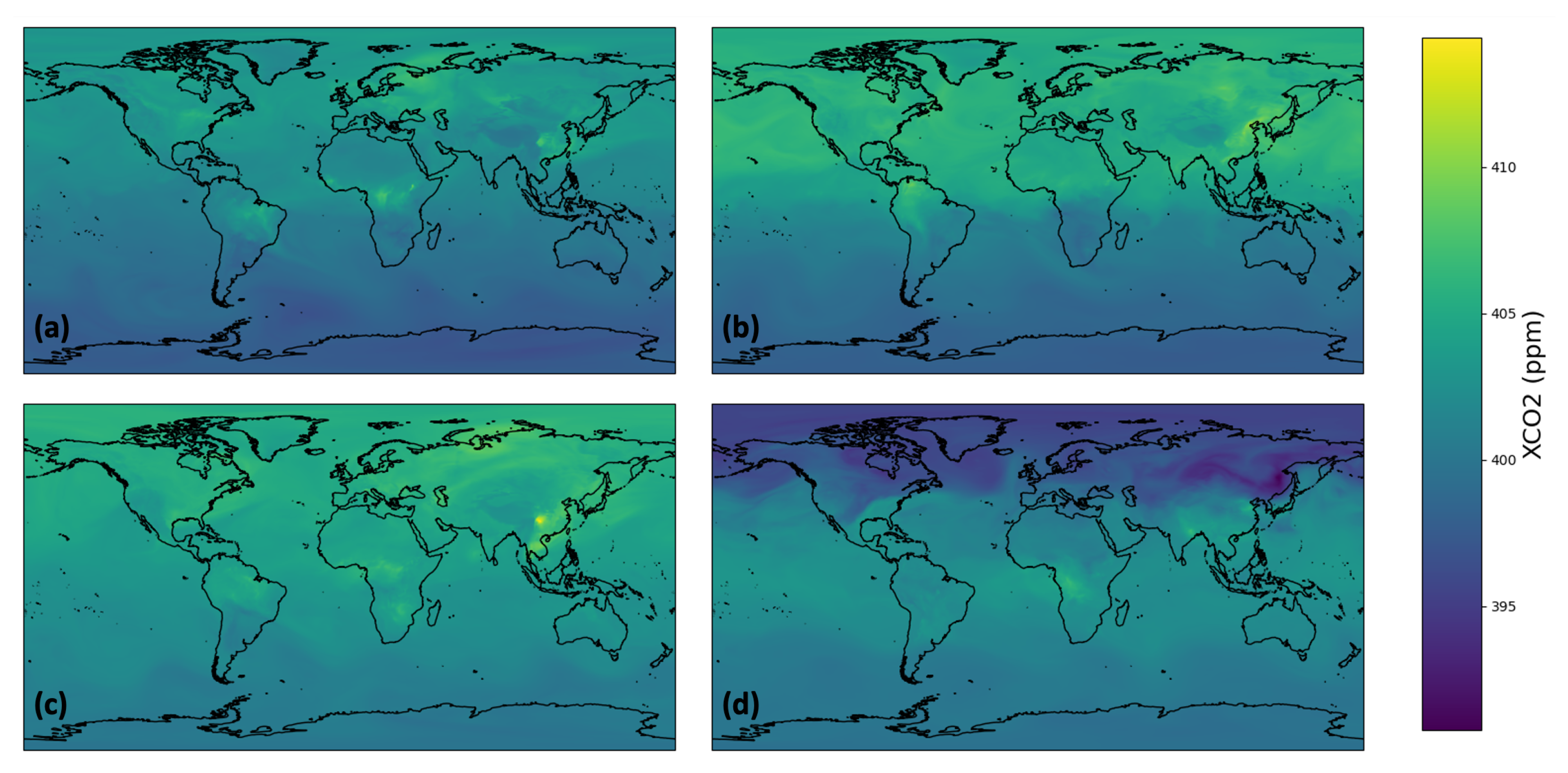
3.1. Dataset Presentation

The super resolution dataset we generated is composed of daily global maps of XCO₂ from 1 January 2015 until 28 February 2022 (see

Table 4. Description of our global super-resolved XCO₂ dataset attributes.

Spatial Resolution (°/km)	Temporal Resolution	Coverage	Timespan
0.03° × 0.04°/3 km × 4 km	1 day	Global	1 January 2015 to 28 February 2022

).

Each map is saved as a numpy array, and the convention we use to name a specific day DD/MM/YYYY is as follows: YYYYMMDD.npy. Figure 5 below contains samples from our dataset.

3.2. Super-Resolved Dataset Evaluation

To assess the quality of our dataset, we compare it against the following global daily datasets: in addition to the original OCO-2 dataset, our comparison includes the dataset from Wang et al. [36], created by combining OCO-2 L2 data with the CAMS reanalysis dataset [57], and a high-resolution dataset derived from OCO-2 L3 data using bicubic interpolation, following the method from Xiang et al. [58] to downscale data coming from of GOSAT. Their attributes are described in

Table 5. Attributes of the additional datasets considered in our benchmark.

Dataset	Spatial Resolution (°/km)	Timespan
OCO-2 dataset (LR)	0.5° × 0.625°/50 km × 70 km	1 January 2015 to 28 February 2022
Bicubic interpolated dataset (BIC)	0.03° × 0.04°/3 km × 4 km	1 January 2015 to 28 February 2022
Fusion dataset (Fus)	0.25° × 0.25°/25 km × 25 km	1 January 2010 to 31 December 2020

below:

Our validation data for this benchmark are XCO₂ estimations from the ground-based spectrometers from the TCCON. Finally, we consider the period between 2015 and 2020 as that is the overlapping period for all the datasets.

3.2.1. General Performance

The main takeaway from the comparison (described in

Table 6. RMSE, R², and MAE from our dataset (SR), the original dataset from OCO-2 (LR), the bicubic interpolated dataset (BIC), and the fusion dataset (Fus.) compared with the TCCON ground-based spectrometers. For each site, the best metric is in bold, while the second-best one is underlined.

Site	RMSE (↓)				R2 (↑)				MAE (↓)
	SR	LR	BIC	Fus.	SR	LR	BIC	Fus.	SR	LR	BIC	Fus.
eu	1.34	1.36	1.32	1.98	0.94	0.94	0.94	0.87	1.01	1.03	0.99	1.60
js	0.96	0.97	0.94	1.21	0.95	0.95	0.95	0.92	0.79	0.80	0.77	1.02
iz	0.59	0.60	0.59	0.65	0.97	0.97	0.97	0.97	0.47	0.48	0.47	0.49
ci	1.26	1.46	1.50	1.09	0.93	0.91	0.91	0.95	1.00	1.19	1.20	0.84
wg	0.80	0.82	0.73	0.83	0.97	0.97	0.97	0.97	0.61	0.63	0.55	0.65
lr	0.62	0.62	0.62	0.77	0.89	0.88	0.88	0.82	0.51	0.52	0.52	0.61
br	0.98	1.00	0.95	1.23	0.97	0.96	0.97	0.95	0.77	0.79	0.74	0.94
sp	1.15	1.18	1.12	1.56	0.95	0.95	0.95	0.91	1.00	1.02	0.96	1.25
ll	0.50	0.50	0.51	0.61	0.96	0.96	0.96	0.95	0.38	0.39	0.39	0.47
pa	0.78	0.77	0.78	1.08	0.98	0.98	0.98	0.96	0.60	0.60	0.61	0.85
hf	1.31	1.48	1.21	1.74	0.84	0.79	0.86	0.71	1.07	1.21	0.99	1.44
jf	1.15	1.38	1.36	1.08	0.80	0.71	0.72	0.83	0.98	1.19	1.18	0.83
ra	0.60	0.60	0.60	0.74	0.98	0.98	0.98	0.97	0.46	0.46	0.46	0.58
et	0.80	0.80	0.82	1.13	0.97	0.97	0.97	0.94	0.63	0.63	0.65	0.90
pr	1.37	1.39	1.37	1.53	0.92	0.91	0.92	0.90	1.09	1.10	1.09	1.20
gm	0.90	0.91	1.05	1.11	0.96	0.96	0.95	0.95	0.71	0.71	0.86	0.86
so	0.91	0.91	0.92	1.46	0.97	0.97	0.97	0.93	0.70	0.71	0.71	1.15
or	1.12	1.12	1.15	1.19	0.95	0.95	0.95	0.94	0.92	0.92	0.95	0.94
bu	0.52	0.52	0.56	0.78	0.96	0.96	0.96	0.91	0.40	0.41	0.43	0.63
df	0.69	0.69	0.65	1.00	0.98	0.98	0.98	0.96	0.54	0.54	0.51	0.81
rj	0.89	0.94	0.83	1.39	0.96	0.96	0.97	0.90	0.66	0.70	0.62	1.09
ka	1.12	1.14	1.19	1.40	0.95	0.95	0.94	0.92	0.92	0.93	0.99	1.11
ni	0.77	0.79	0.79	1.06	0.89	0.89	0.88	0.79	0.65	0.67	0.67	0.87
db	0.71	0.70	0.70	0.93	0.98	0.98	0.98	0.96	0.56	0.56	0.55	0.72
Avg.	0.92	0.94	0.94	1.12	0.97	0.96	0.96	0.95	0.70	0.72	0.72	0.85

) is that our model is able to increase the resolution of the OCO-2 dataset 16 times while preserving the quality of the data. Averaged over all members of the TCCON, our super-resolved dataset presents a lower RMSE (0.92) than the original dataset (0.94). As the RMSE is known to penalize larger errors more severely [59], the table shows that our model does not introduce significant errors to the estimations from the OCO-2 dataset. Similarly, the MAE results highlight that, on average, our model predicts values closer to the ground truth, indicating that the downscaling improves, albeit modestly, the estimations. Our dataset also reports the best average value for the coefficient of determination R², which emphasizes that the variations of XCO₂ are well described by our super resolution model. On the other hand, the fusion dataset is consistently outperformed by the other datasets. This is reflected in the row of average RMSE and MAE, where its estimations are approximately 20% worse than our super-resolved dataset.

3.2.2. Location-Specific Performance

These findings remain consistent when transitioning from broad to site-specific observations. Over all metrics (RMSE, R², and MAE), the estimations generated by our model are best or second best on all sites, underlining its consistency. We also note that the choice of downscaling method matters. Our dataset and bicubic interpolation provide the best estimations compared with the TCCON validation data (described in Section 2.2) in approximately the same number of locations. However, our method is never outperformed by the original dataset if we consider the R² and MAE and in only two locations if we consider the RMSE. In contrast, the interpolated dataset performs worse in nine, three, and seven locations for the RMSE, R², and MAE respectively, making it unreliable on a global scale. The fusion dataset underperforms again, providing the best estimations in only two locations and the worst ones in all other sites.

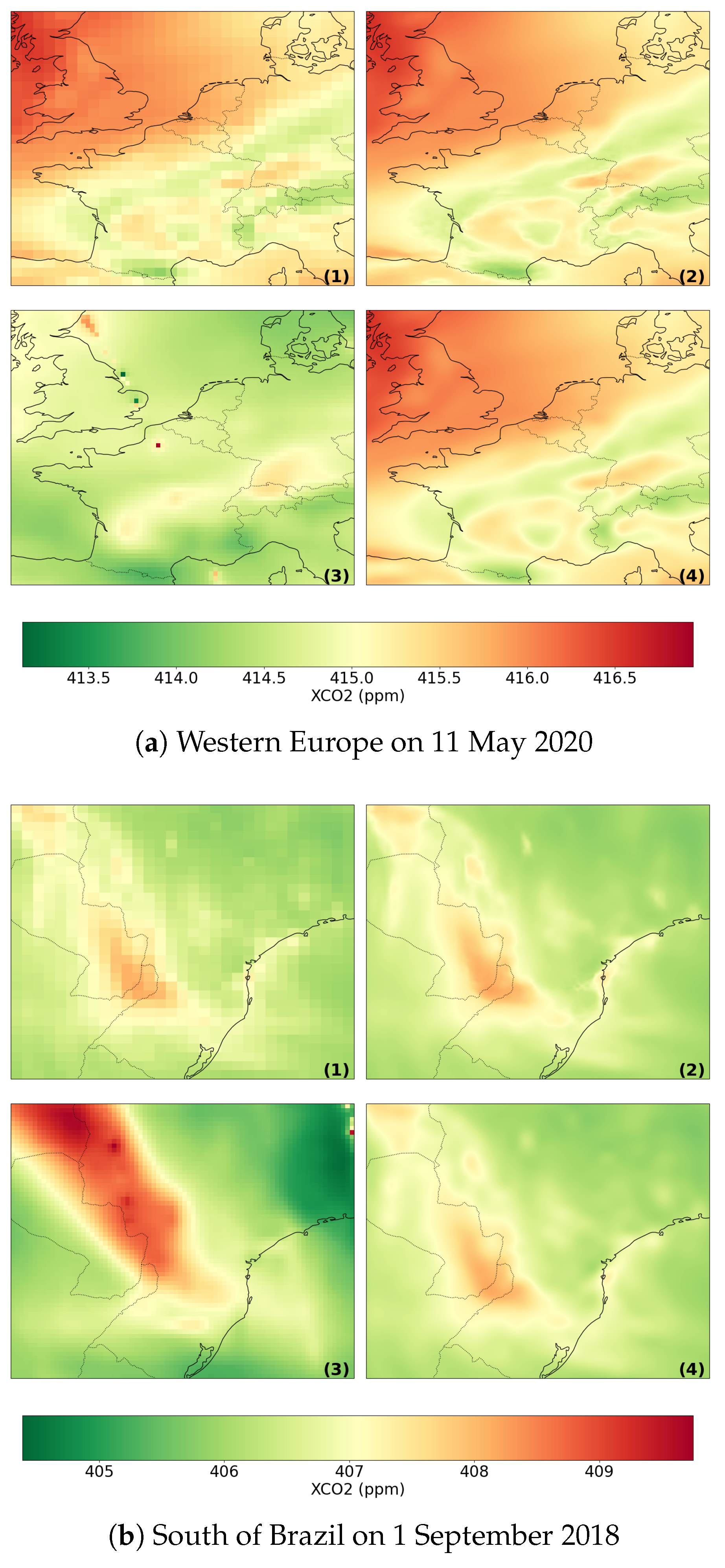
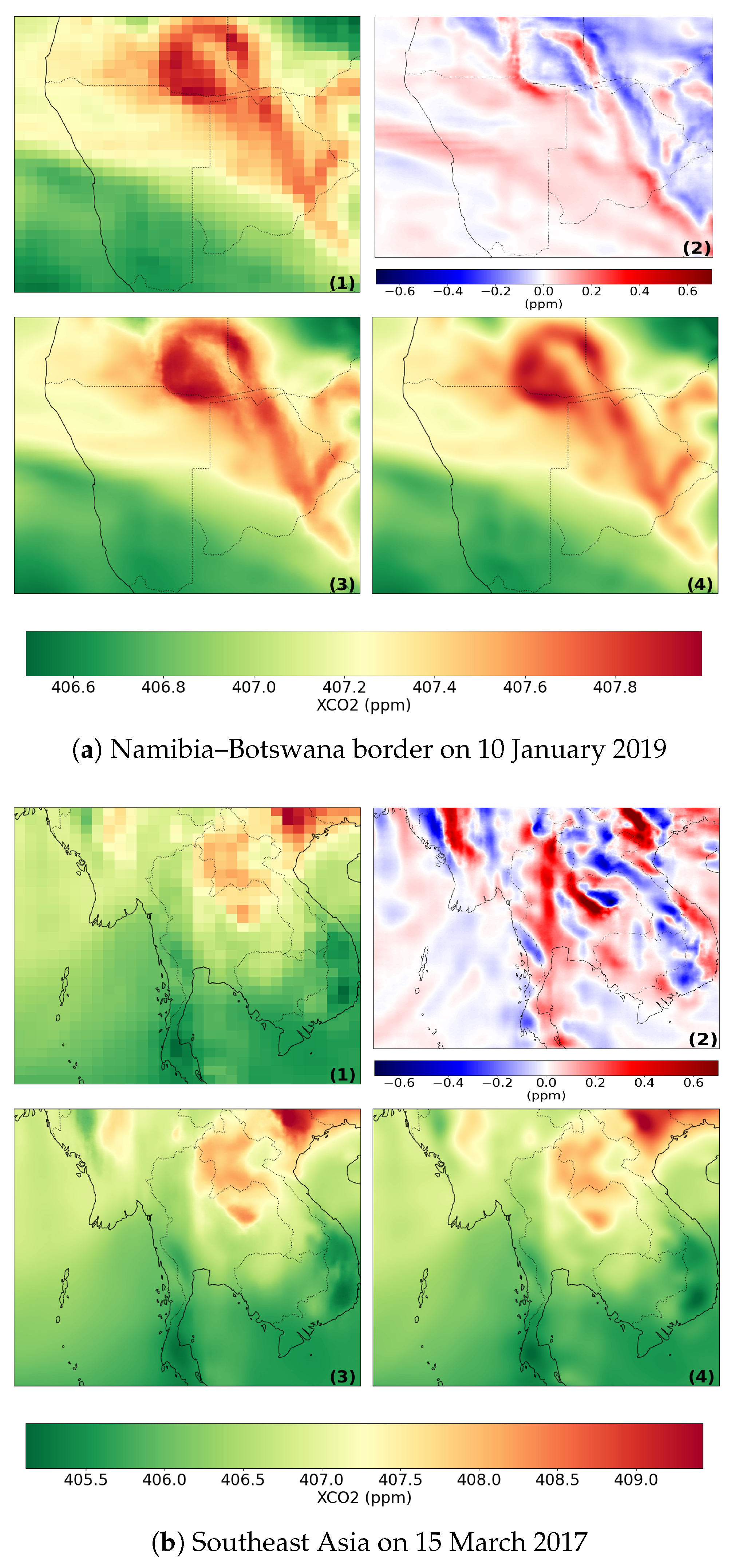
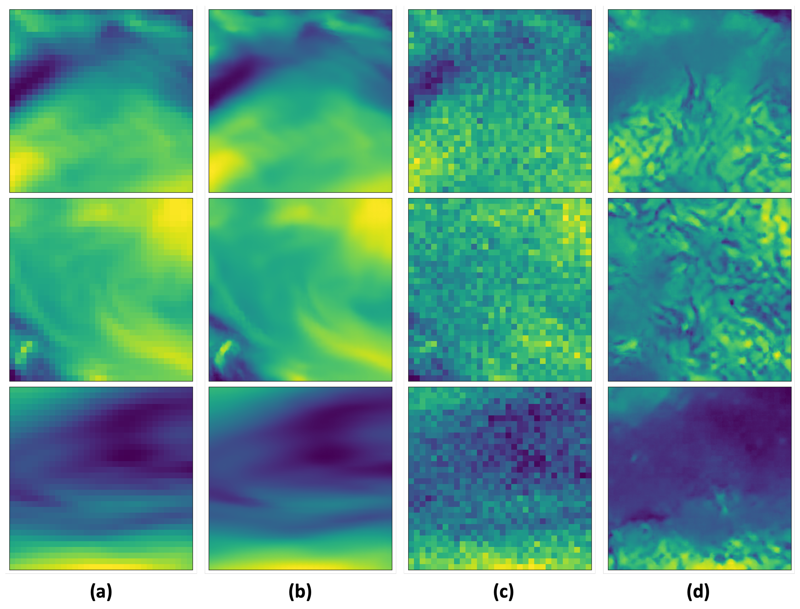
3.2.3. Visual Confirmation

Samples from each dataset over Western Europe in May 2020 and over Brazil in September 2018 are presented in Figure 6. There is a significant discrepancy between the fusion dataset and the other three datasets. This confirms the analysis stemming from Table 6. In Figure 6a, we observe isolated sites of high or low CO₂ concentration in the north of France and the United Kingdom. These spots may arise from the fusion of multiple datasets but appear erroneous. In Figure 6b, the high concentration zone following the border between Brazil and Paraguay is well encapsulated by all methods, although it appears more intense in the fusion dataset. When inspecting our super-resolved map, we see that the small patches of high concentration have a more distinct shape and appear less blurry than when interpolated using bicubic interpolation, although they are not clearly visible. To mitigate the bias introduced by the fusion dataset, which stretches the color bar in high and low values, and further highlight the differences between our dataset and the bicubic interpolation, we present maps of the Namibia–Botswana border in January 2019 and Southeast Asia in March 2017 in Figure 7. We clearly recognize the issues with bicubic interpolation, where high gradients are often flattened to produce smoother transitions [60] between regions of high and low concentration. In Figure 7a, this effect is evident in areas with sharp increase (respectively decrease) in CO₂ concentration, where our dataset provides significantly higher (lower) estimations than the interpolated dataset.

As a result, some information may be lost in the bicubic interpolation dataset as it underestimates CO₂ concentration in high pollution areas but overestimates it in low pollution areas.

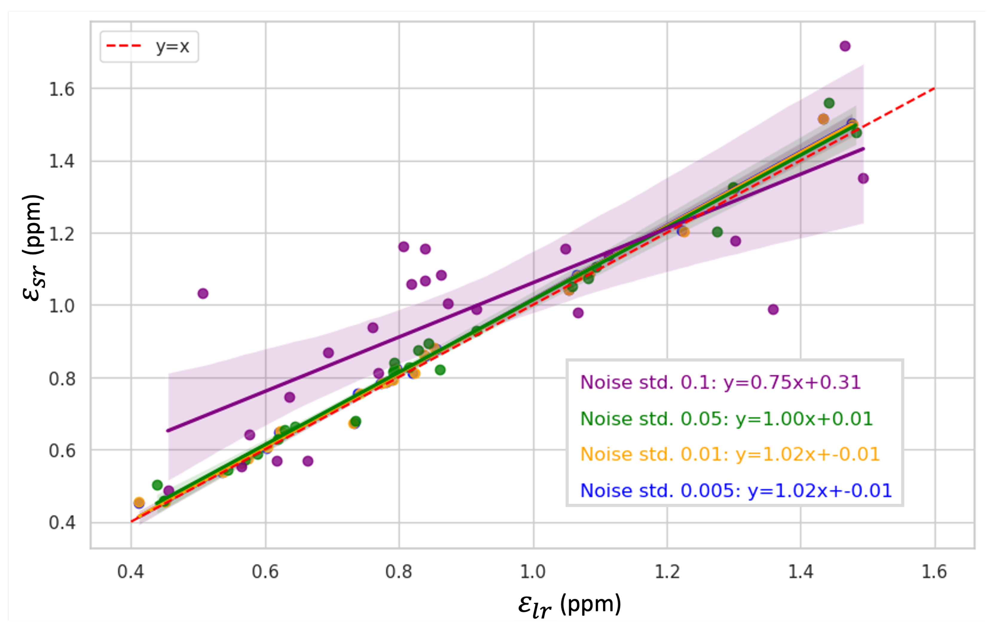
3.3. Model Uncertainty

In this section, we evaluate the uncertainty in our super resolution model. To do so, we analyze the propagation of a perturbation $\delta$ added to the low-resolution XCO₂ data before downscaling. This noise follows the following distribution:

$$\delta \sim \mathcal{N}(\mathbf{0},\sigma \mathbf{I})$$

(7)

where $\sigma$ is the standard deviation of the noise and $\mathbf{I}$ is the identity matrix sharing the same dimension as our model inputs. Let ${\tilde{x}}_{LS}$ be the perturbed data.

$${\tilde{x}}_{LS}=x_{LS}+\delta$$

(8)

For a ground-based spectrometer of the TCCON, we then define ${\epsilon }_{ls}$ as the error between the perturbed low-resolution estimation ${\tilde{x}}_{LS}^{sensor}$ and the spectrometers’ estimation y, which we again consider as ground truth, as follows:

$${\epsilon }_{lr}={\tilde{x}}_{LS}^{sensor}-y$$

(9)

Given ${\tilde{x}}_{SR}$ as the output of the super resolution model F when noise is added,

$${\tilde{x}}_{SR}=F\left({\tilde{x}}_{LS}\right)$$

(10)

We are therefore interested in evaluating the error ${\epsilon }_{sr}$ (defined in Equation (11)) and its relationship with ${\epsilon }_{lr}$.

$${\epsilon }_{sr}={\tilde{x}}_{SR}^{sensor}-y.$$

(11)

Figure 8 below depicts how noise affects ${\epsilon }_{lr}$ and ${\epsilon }_{sr}$. We can observe that both variables remain similar until the noise becomes too important ($\sigma >0.05$) and drowns the original information (see Figure 9). This indicates that our model does not propagate small errors, which in turn suggests that it is able to denoise, at least partially, the data while it performs super resolution. Another result worth mentioning is that, for very noisy low resolution maps (represented by purple dots in Figure 8), our super resolution model tends to increase ${\epsilon }_{sr}$ for ${\epsilon }_{lr}$ < 1 ppm, while for higher values of ${\epsilon }_{lr}$ (>1 ppm), the resulting error in XCO₂ estimation can decrease, i.e., ${\epsilon }_{sr}<{\epsilon }_{lr}$.

Finally, Figure 9 represents what happens when the low-resolution input becomes so noisy that too little information remains: the model is not able to generate a conclusive high-resolution XCO₂ map, and even low-frequency details in the low-resolution input map are lost.

3.4. Application: Observation of Localized Changes in Pollution Through the COVID-19 Pandemic

In this section, we propose a use case designed to demonstrate the versatility of our dataset in identifying both global and local fluctuations in CO₂ concentration, specifically within the context of the coronavirus disease (COVID-19) pandemic. The COVID-19 pandemic caused by SARS-CoV-2 (severe acute respiratory syndrome coronavirus 2) [61] has significantly impacted human societies from late 2019 until several months into 2021 [62]. Lockdowns, short-term factory closures, and a massive reduction in air travel [63] have resulted in a global drop in CO₂ emissions. Figure 10 highlights the impact this drop in emissions had on CO₂ concentration during 2020.

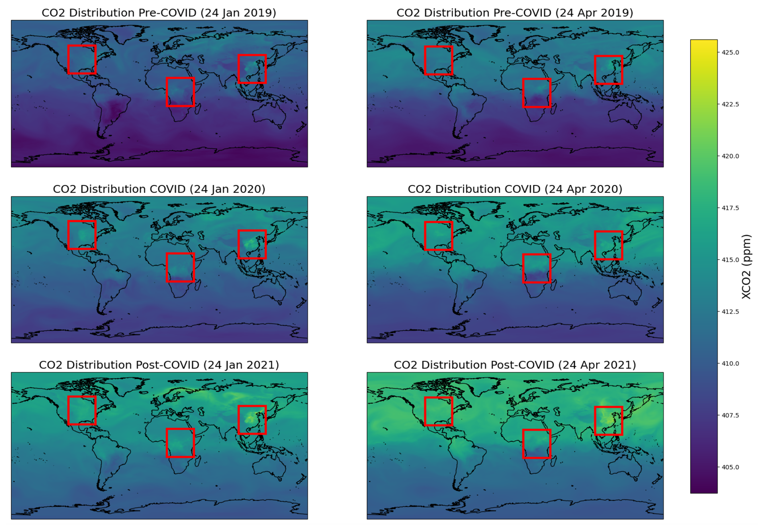
3.4.1. Global CO₂ Trends

The figure first confirms the global rise of CO₂ concentration over the years, which has been noted in other studies [64,65]. In 2019, we see that the average CO₂ concentration in the southern hemisphere is around 408 ppm. It steadily increases to reach around 415 ppm at the end of 2021. This trend is even more apparent in the northern hemisphere, where the CO₂ concentration was rarely above 417 ppm in early 2020 before some areas reached well above 420 ppm at the end of 2021.

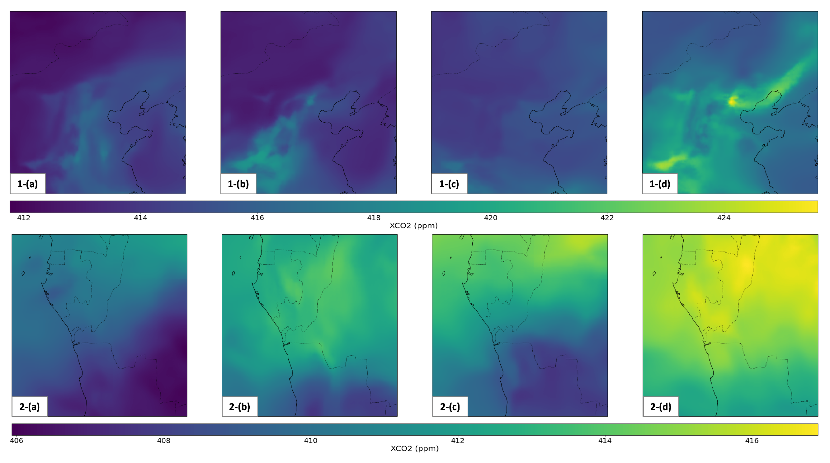
3.4.2. Local Variations

A second observation is the visible impact that governments’ responses to the pandemic [66] had on regional levels of CO₂ concentration in mid-2020. The areas delimited by the red triangles in North America, Africa, and East Asia on Figure 10 are usually regional spots of high concentration, as can be seen in 2019 and 2021. It appears that these spots are far less prominent in terms of CO₂ concentration relatively to their surroundings in April 2020. They stand out again in 2021, indicating a return to pre-pandemic behavior. This is more distinctly observable in Figure 11: usual spots of high pollution in Hebei and Henan (China), southwest of Beijing, are absent in Figure 11(1-(c)), corresponding to April 2020, probably due to lockdowns and a drop in activity for most factories. The second row of Figure 11 also highlights this reduction in pollution in the southern part of the Democratic Republic of Congo (DRC), following the DRC–Angola border. The stark contrast between Figure 11(2-(c)) in April 2020 and Figure 11(2-(d)) in January 2021 illustrates human activity coming to a standstill and then resuming to “normal”, highlighting the impact it has on CO₂ concentration.

4. Discussion

Our results show that our super resolution model is able to downscale the OCO-2 dataset without compromising the quality of the estimations. Through our validation with the TCCON and our visualizations, we demonstrate that our dataset yields better local estimations, a superior resolution, and more plausible-looking maps compared with existing products from alternative reconstruction approaches. However, we highlight here a few areas worth investigating in future works. Currently, only the low-resolution dataset serves as reference to create super-resolved maps. It is potentially relevant to consider additional geographical features to guide the downscaling process [67]. By adjusting our approach to allow multiple inputs, our model could gain further insights from the added data, leading to better estimations. A complementary approach involves integrating physical constraints into the model [68,69], ensuring that the super-resolved maps adhere in a more explicit way to the laws of physics, which would in turn generate more realistic global fields.

A major issue our model could face in the future is the distribution shift [70], which is common for deep learning models applied to real-world problems. This shift occurs on the target domain of our data, in our case, XCO₂ data. With the continuous rise of CO₂ concentration in the atmosphere, the quality of our super-resolved maps could decrease as the new distribution of XCO₂ will not necessarily match the data distribution our model has been trained on. Different methods are available to retrain the model: a new existing training dataset with a better matching distribution, an adapted sampling of the training dataset, called weighted resampling [71], to match the new target distribution, or even the generation of synthetic training data [72]. Inference time is another area of importance for real-world applications such as air quality prediction [73] or wildfire monitoring [74]). In such scenarios, running a simulation or generating a dataset needs to be performed near real time. For example, air quality predictions need to be updated hourly and with a fine spatial granularity. In this context, our super resolution model can generate high spatial resolution XCO₂ maps of area of interest almost instantly without having to involve physics-based models or integrate multiple datasets like the methods described in Section 3, which can be an advantage to potentially help the air quality prediction.

5. Conclusions

In this paper, we present a new global high-resolution daily dataset of atmospheric CO₂ concentration. To generate this dataset, we downscale L3 products from NASA using super resolution and manage to increase the spatial resolution of the original dataset 16 times while maintaining, and even marginally improving, its precision. The lack of high-resolution CO₂ datasets renders supervised learning methods impractical as the direct mapping between low and high CO₂ concentration maps remains inaccessible. During training, our super resolution model therefore learns to reconstruct high-resolution temperature data that were previously upscaled. We explain the theoretical validity of using another physical variable for training and then transfer to CO₂ by establishing that, once normalized, our training and target datasets share similar distributions. We release this dataset and hope that it will provide new opportunities for global CO₂ monitoring. We highlight how it can be used to monitor singular global scale events, like the COVID-19 pandemic, while also capturing local or regional changes. Finally, the global nature of each map represents a significant advancement in achieving a more consistent monitoring across different regions and thus reduces the disparities stemming from insufficient infrastructure.

References

1. Core Writing Team; Lee, H.; Romero, J. Synthesis Report. Contribution of Working Groups I, II and III to the Sixth Assessment Report of the Intergovernmental Panel on Climate Change. In Climate Change 2023: Synthesis Report, Proceedings of the Panel’s 58th Session, Interlaken, Switzerland, 13-19 March 2023; IPCC: Geneva, Switzerland, 2023. [Google Scholar] [CrossRef]
2. United Nations. Paris Agreement; United Nations: New York City, NY, USA, 2015. [Google Scholar]
3. United Nations Environment Programme. Global Resources Outlook 2024: Bend the Trend—Pathways to a Liveable Planet as Resource Use Spikes. International Resource Panel. Nairobi. 2024. Available online: https://www.unep.org/resources/Global-Resource-Outlook-2024 (accessed on 15 January 2025).
4. Naumann, G.; Cammalleri, C.; Mentaschi, L.; Feyen, L. Increased economic drought impacts in Europe with anthropogenic warming. Nat. Clim. Change 2021, 11, 485–491. [Google Scholar] [CrossRef]
5. Ou, Y.; Iyer, G.; Fawcett, A.; Hultman, N.; McJeon, H.; Ragnauth, S.; Smith, S.J.; Edmonds, J. Role of non-CO2 greenhouse gas emissions in limiting global warming. One Earth 2022, 5, 1312–1315. [Google Scholar] [CrossRef] [PubMed]
6. Weiss, R.F.; Prinn, R.G. Quantifying greenhouse-gas emissions from atmospheric measurements: A critical reality check for climate legislation. Philos. Trans. R. Soc. A Math. Phys. Eng. Sci. 2011, 369, 1925–1942. [Google Scholar] [CrossRef]
7. Jarnicka, J.; Żebrowski, P. Learning in greenhouse gas emission inventories in terms of uncertainty improvement over time. Mitig. Adapt. Strateg. Glob. Change 2019, 24, 1143–1168. [Google Scholar] [CrossRef]
8. Wunch, D.; Toon, G.C.; Blavier, J.F.L.; Washenfelder, R.A.; Notholt, J.; Connor, B.J.; Griffith, D.W.; Sherlock, V.; Wennberg, P.O. The total carbon column observing network. Philos. Trans. R. Soc. A Math. Phys. Eng. Sci. 2011, 369, 2087–2112. [Google Scholar] [CrossRef]
9. Kasuya, M.; Nakajima, M.; Hamazaki, T. Greenhouse gases observing satellite (GOSAT) program overview and its development status. Trans. Jpn. Soc. Aeronaut. Space Sci. Space Technol. Jpn. 2009, 7, To_4_5–To_4_10. [Google Scholar] [CrossRef]
10. Eldering, A.; Boland, S.; Solish, B.; Crisp, D.; Kahn, P.; Gunson, M. High precision atmospheric CO2 measurements from space: The design and implementation of OCO-2. In Proceedings of the 2012 IEEE Aerospace Conference, Big Sky, MT, USA, 3–10 March 2012; pp. 1–10. [Google Scholar]
11. Eldering, A.; Taylor, T.E.; O’Dell, C.W.; Pavlick, R. The OCO-3 mission: Measurement objectives and expected performance based on 1 year of simulated data. Atmos. Meas. Tech. 2019, 12, 2341–2370. [Google Scholar] [CrossRef]
12. Nassar, R.; Mastrogiacomo, J.P.; Bateman-Hemphill, W.; McCracken, C.; MacDonald, C.G.; Hill, T.; O’Dell, C.W.; Kiel, M.; Crisp, D. Advances in quantifying power plant CO2 emissions with OCO-2. Remote Sens. Environ. 2021, 264, 112579. [Google Scholar] [CrossRef]
13. Lopez, F.P.A.; Zhou, G.; Jing, G.; Zhang, K.; Tan, Y. XCO2 and XCH4 Reconstruction Using GOSAT Satellite Data Based on EOF-Algorithm. Remote Sens. 2022, 14, 2622. [Google Scholar] [CrossRef]
14. Hu, K.; Liu, Z.; Shao, P.; Ma, K.; Xu, Y.; Wang, S.; Wang, Y.; Wang, H.; Di, L.; Xia, M.; et al. A review of satellite-based CO2 data reconstruction studies: Methodologies, challenges, and advances. Remote Sens. 2024, 16, 3818. [Google Scholar] [CrossRef]
15. He, Z.; Lei, L.; Zhang, Y.; Sheng, M.; Wu, C.; Li, L.; Zeng, Z.C.; Welp, L.R. Spatio-temporal mapping of multi-satellite observed column atmospheric CO2 using precision-weighted kriging method. Remote Sens. 2020, 12, 576. [Google Scholar] [CrossRef]
16. Zammit-Mangion, A.; Cressie, N.; Shumack, C. On Statistical Approaches to Generate Level 3 Products from Satellite Remote Sensing Retrievals. Remote Sens. 2018, 10, 155. [Google Scholar] [CrossRef]
17. Jacobson, A.R.; Schuldt, K.N.; Tans, P. CarbonTracker CT2022; NOAA Global Monitoring Laboratory: Boulder, CO, USA, 2023.
18. Eastham, S.D.; Long, M.S.; Keller, C.A.; Lundgren, E.; Yantosca, R.M.; Zhuang, J.; Li, C.; Lee, C.J.; Yannetti, M.; Auer, B.M.; et al. GEOS-Chem High Performance (GCHP v11-02c): A next-generation implementation of the GEOS-Chem chemical transport model for massively parallel applications. Geosci. Model Dev. 2018, 11, 2941–2953. [Google Scholar] [CrossRef]
19. Van Der Woude, A.M.; De Kok, R.; Smith, N.; Luijkx, I.T.; Botía, S.; Karstens, U.; Kooijmans, L.M.; Koren, G.; Meijer, H.A.; Steeneveld, G.J.; et al. Near-real-time CO2 fluxes from CarbonTracker Europe for high-resolution atmospheric modeling. Earth Syst. Sci. Data 2023, 15, 579–605. [Google Scholar] [CrossRef]
20. Hu, K.; Zhang, Q.; Feng, X.; Liu, Z.; Shao, P.; Xia, M.; Ye, X. An Interpolation and Prediction Algorithm for XCO2 based on Multi-source Time Series Data. Remote Sens. 2024, 16, 1907. [Google Scholar] [CrossRef]
21. Rodriguez-Perez, D.; Sanchez-Carnero, N. Multigrid/multiresolution interpolation: Reducing oversmoothing and other sampling effects. Geomatics 2022, 2, 236–253. [Google Scholar] [CrossRef]
22. Goodfellow, I.; Bengio, Y.; Courville, A.; Bengio, Y. Deep Learning; MIT Press: Cambridge, MA, USA, 2016; Volume 1. [Google Scholar]
23. He, C.; Ji, M.; Li, T.; Liu, X.; Tang, D.; Zhang, S.; Luo, Y.; Grieneisen, M.L.; Zhou, Z.; Zhan, Y. Deriving Full-Coverage and Fine-Scale XCO2 Across China Based on OCO-2 Satellite Retrievals and CarbonTracker Output. Geophys. Res. Lett. 2022, 49, e2022GL098435. [Google Scholar] [CrossRef]
24. Ke, G.; Meng, Q.; Finley, T.; Wang, T.; Chen, W.; Ma, W.; Ye, Q.; Liu, T.Y. Lightgbm: A highly efficient gradient boosting decision tree. In Proceedings of the Advances in Neural Information Processing Systems, Long Beach, CA, USA, 4–9 December 2017; Volume 30. [Google Scholar]
25. Siabi, Z.; Falahatkar, S.; Alavi, S.J. Spatial distribution of XCO2 using OCO-2 data in growing seasons. J. Environ. Manag. 2019, 244, 110–118. [Google Scholar] [CrossRef]
26. Taud, H.; Mas, J.F. Multilayer perceptron (MLP). In Geomatic Approaches for Modeling Land Change Scenarios; Springer: Berlin/Heidelberg, Germany, 2017; pp. 451–455. [Google Scholar]
27. Moser, B.B.; Raue, F.; Frolov, S.; Palacio, S.; Hees, J.; Dengel, A. Hitchhiker’s Guide to Super-Resolution: Introduction and Recent Advances. IEEE Trans. Pattern Anal. Mach. Intell. 2023, 45, 9862–9882. [Google Scholar] [CrossRef]
28. Saharia, C.; Ho, J.; Chan, W.; Salimans, T.; Fleet, D.J.; Norouzi, M. Image Super-Resolution via Iterative Refinement. IEEE Trans. Pattern Anal. Mach. Intell. 2023, 45, 4713–4726. [Google Scholar] [CrossRef]
29. Lever, J.; Cheng, S.; Casas, C.Q.; Liu, C.; Fan, H.; Platt, R.; Rakotoharisoa, A.; Johnson, E.; Li, S.; Shang, Z.; et al. Facing & mitigating common challenges when working with real-world data: The Data Learning Paradigm. J. Comput. Sci. 2025, 85, 102523. [Google Scholar]
30. Wang, P.; Bayram, B.; Sertel, E. A comprehensive review on deep learning based remote sensing image super-resolution methods. Earth-Sci. Rev. 2022, 232, 104110. [Google Scholar] [CrossRef]
31. Haris, M.; Shakhnarovich, G.; Ukita, N. Deep Back-ProjectiNetworks for Single Image Super-Resolution. IEEE Trans. Pattern Anal. Mach. Intell. 2021, 43, 4323–4337. [Google Scholar] [CrossRef] [PubMed]
32. Goodfellow, I.; Pouget-Abadie, J.; Mirza, M.; Xu, B.; Warde-Farley, D.; Ozair, S.; Courville, A.; Bengio, Y. Generative adversarial networks. Commun. ACM 2020, 63, 139–144. [Google Scholar] [CrossRef]
33. Vaswani, A. Attention is all you need. In Advances in Neural Information Processing Systems; MIT Press: Cambridge, MA, USA, 2017. [Google Scholar]
34. Sheng, M.; Lei, L.; Zeng, Z.C.; Rao, W.; Song, H.; Wu, C. Global land 1° mapping dataset of XCO2 from satellite observations of GOSAT and OCO-2 from 2009 to 2020. Big Earth Data 2022, 7, 170–190. [Google Scholar] [CrossRef]
35. Weir, B.; Ott, L.; OCO-2 Science Team. OCO-2 GEOS Level 3 Daily, 0.5 × 0.625 Assimilated CO2 V10r; Goddard Earth Sciences Data and Information Services Center (GES DISC): Severna Park, MD, USA, 2022.
36. Wang, Y.; Yuan, Q.; Li, T.; Yang, Y.; Zhou, S.; Zhang, L. Seamless mapping of long-term (2010–2020) daily global XCO2 and XCH4 from the Greenhouse Gases Observing Satellite (GOSAT), Orbiting Carbon Observatory 2 (OCO-2), and CAMS global greenhouse gas reanalysis (CAMS-EGG4) with a spatiotemporally self-supervised fusion method. Earth Syst. Sci. Data 2023, 15, 3597–3622. [Google Scholar] [CrossRef]
37. Li, J.; Jia, K.; Wei, X.; Xia, M.; Chen, Z.; Yao, Y.; Zhang, X.; Jiang, H.; Yuan, B.; Tao, G.; et al. High-spatiotemporal resolution mapping of spatiotemporally continuous atmospheric CO2 concentrations over the global continent. Int. J. Appl. Earth Obs. Geoinf. 2022, 108, 102743. [Google Scholar] [CrossRef]
38. Taylor, T.E.; O’Dell, C.W.; Baker, D.; Bruegge, C.; Chang, A.; Chapsky, L.; Chatterjee, A.; Cheng, C.; Chevallier, F.; Crisp, D.; et al. Evaluating the consistency between OCO-2 and OCO-3 XCO2 estimates derived from the NASA ACOS version 10 retrieval algorithm. Atmos. Meas. Tech. Discuss. 2023, 16, 3173–3209. [Google Scholar] [CrossRef]
39. Parker, R.; Boesch, H.; Cogan, A.; Fraser, A.; Feng, L.; Palmer, P.I.; Messerschmidt, J.; Deutscher, N.; Griffith, D.W.; Notholt, J.; et al. Methane observations from the Greenhouse Gases Observing SATellite: Comparison to ground-based TCCON data and model calculations. Geophys. Res. Lett. 2011, 38, L15807. [Google Scholar] [CrossRef]
40. Sha, M.K.; De Mazière, M.; Notholt, J.; Blumenstock, T.; Chen, H.; Dehn, A.; Griffith, D.W.; Hase, F.; Heikkinen, P.; Hermans, C.; et al. Intercomparison of low- and high-resolution infrared spectrometers for ground-based solar remote sensing measurements of total column concentrations of CO2, CH4, and CO. Atmos. Meas. Tech. 2020, 13, 4791–4839. [Google Scholar] [CrossRef]
41. Zhou, M.; Langerock, B.; Vigouroux, C.; Sha, M.K.; Hermans, C.; Metzger, J.M.; Chen, H.; Ramonet, M.; Kivi, R.; Heikkinen, P.; et al. TCCON and NDACC X CO measurements: Difference, discussion and application. Atmos. Meas. Tech. 2019, 12, 5979–5995. [Google Scholar] [CrossRef]
42. Xiong, X.; Chiang, K.; Sun, J.; Barnes, W.; Guenther, B.; Salomonson, V. NASA EOS Terra and Aqua MODIS on-orbit performance. Adv. Space Res. 2009, 43, 413–422. [Google Scholar] [CrossRef]
43. Wan, Z.; Hook, S.; Hulley, G. MODIS/Terra Land Surface Temperature/Emissivity Daily L3 global 0.05 Deg CMG V061 [Data Set]; NASA EOSDIS Land Processes DAAC: Sioux Falls, SD, USA, 2021.
44. Zhuang, F.; Qi, Z.; Duan, K.; Xi, D.; Zhu, Y.; Zhu, H.; Xiong, H.; He, Q. A comprehensive survey on transfer learning. Proc. IEEE 2020, 109, 43–76. [Google Scholar]
45. Haut, J.M.; Fernandez-Beltran, R.; Paoletti, M.E.; Plaza, J.; Plaza, A.; Pla, F. A new deep generative network for unsupervised remote sensing single-image super-resolution. IEEE Trans. Geosci. Remote Sens. 2018, 56, 6792–6810. [Google Scholar] [CrossRef]
46. Wei, Y.; Gu, S.; Li, Y.; Timofte, R.; Jin, L.; Song, H. Unsupervised real-world image super resolution via domain-distance aware training. In Proceedings of the IEEE/CVF Conference on Computer Vision and Pattern Recognition, Nashville, TN, USA, 20–25 June 2021; pp. 13385–13394. [Google Scholar]
47. Timofte, R.; Gu, S.; Wu, J.; Van Gool, L.; Zhang, L.; Yang, M.H.; Haris, M.; Shakhnarovich, G.; Ukita, N.; Hu, S.; et al. NTIRE 2018 Challenge on Single Image Super-Resolution: Methods and Results. In Proceedings of the IEEE Conference on Computer Vision and Pattern Recognition (CVPR) Workshops, Salt Lake City, UT, USA, 18–22 June 2018; pp. 114–125. [Google Scholar]
48. Xia, G.S.; Bai, X.; Ding, J.; Zhu, Z.; Belongie, S.; Luo, J.; Datcu, M.; Pelillo, M.; Zhang, L. DOTA: A large-scale dataset for object detection in aerial images. In Proceedings of the IEEE Conference on Computer Vision and Pattern Recognition, Salt Lake City, UT, USA, 18–23 June 2018; pp. 3974–3983. [Google Scholar]
49. Zhang, M.; Kafy, A.A.; Xiao, P.; Han, S.; Zou, S.; Saha, M.; Zhang, C.; Tan, S. Impact of urban expansion on land surface temperature and carbon emissions using machine learning algorithms in Wuhan, China. Urban Clim. 2023, 47, 101347. [Google Scholar] [CrossRef]
50. Zhao, J.; Zhang, S.; Yang, K.; Zhu, Y.; Ma, Y. Spatio-temporal variations of CO2 emission from energy consumption in the yangtze river delta region of china and its relationship with nighttime land surface temperature. Sustainability 2020, 12, 8388. [Google Scholar] [CrossRef]
51. Hong, T.; Huang, X.; Zhang, X.; Deng, X. Correlation modelling between land surface temperatures and urban carbon emissions using multi-source remote sensing data: A case study. Phys. Chem. Earth Parts A/B/C 2023, 132, 103489. [Google Scholar] [CrossRef]
52. Dong, R.; Zhang, L.; Fu, H. RRSGAN: Reference-based super-resolution for remote sensing image. IEEE Trans. Geosci. Remote Sens. 2021, 60, 5601117. [Google Scholar] [CrossRef]
53. Soh, J.W.; Cho, S.; Cho, N.I. Meta-transfer learning for zero-shot super-resolution. In Proceedings of the IEEE/CVF Conference on Computer Vision and Pattern Recognition, Seattle, WA, USA, 14–19 June 2020; pp. 3516–3525. [Google Scholar]
54. Dai, S.; Han, M.; Wu, Y.; Gong, Y. Bilateral back-projection for single image super resolution. In Proceedings of the 2007 IEEE International Conference on Multimedia and Expo, Beijing, China, 2–5 July 2007; pp. 1039–1042. [Google Scholar]
55. Wang, W.; Zhang, H.; Yuan, Z.; Wang, C. Unsupervised real-world super-resolution: A domain adaptation perspective. In Proceedings of the IEEE/CVF International Conference on Computer Vision, Montreal, BC, Canada, 11–17 October 2021; pp. 4318–4327. [Google Scholar]
56. Muthukumar, P.; Cocom, E.; Nagrecha, K.; Comer, D.; Burga, I.; Taub, J.; Calvert, C.F.; Holm, J.; Pourhomayoun, M. Predicting PM2.5 atmospheric air pollution using deep learning with meteorological data and ground-based observations and remote-sensing satellite big data. Air Qual. Atmos. Health 2022, 15, 1221–1234. [Google Scholar] [CrossRef]
57. Agustí-Panareda, A.; Barré, J.; Massart, S.; Inness, A.; Aben, I.; Ades, M.; Baier, B.C.; Balsamo, G.; Borsdorff, T.; Bousserez, N.; et al. Technical note: The CAMS greenhouse gas reanalysis from 2003 to 2020. Atmos. Chem. Phys. 2023, 23, 3829–3859. [Google Scholar] [CrossRef]
58. Xiang, R.; Yang, H.; Yan, Z.; Taha, A.M.M.; Xu, X.; Wu, T. Super-resolution reconstruction of GOSAT CO2 products using bicubic interpolation. Geocarto Int. 2022, 37, 15187–15211. [Google Scholar] [CrossRef]
59. Hodson, T.O. Root mean square error (RMSE) or mean absolute error (MAE): When to use them or not. Geosci. Model Dev. Discuss. 2022, 14, 5481–5487. [Google Scholar] [CrossRef]
60. Biau, G.; Zorita, E.; von Storch, H.; Wackernagel, H. Estimation of precipitation by kriging in the EOF space of thesea level pressure field. J. Clim. 1999, 12, 1070–1085. [Google Scholar] [CrossRef]
61. Ge, H.; Wang, X.; Yuan, X.; Xiao, G.; Wang, C.; Deng, T.; Yuan, Q.; Xiao, X. The epidemiology and clinical information about COVID-19. Eur. J. Clin. Microbiol. Infect. Dis. 2020, 39, 1011–1019. [Google Scholar] [CrossRef]
62. Carvalho, T.; Krammer, F.; Iwasaki, A. The first 12 months of COVID-19: A timeline of immunological insights. Nat. Rev. Immunol. 2021, 21, 245–256. [Google Scholar] [CrossRef]
63. Muhammad, S.; Long, X.; Salman, M. COVID-19 pandemic and environmental pollution: A blessing in disguise? Sci. Total Environ. 2020, 728, 138820. [Google Scholar] [CrossRef]
64. Yin, S.; Wang, X.; Tani, H.; Zhang, X.; Zhong, G.; Sun, Z.; Chittenden, A.R. Analyzing temporo-spatial changes and the distribution of the CO2 concentration in Australia from 2009 to 2016 by greenhouse gas monitoring satellites. Atmos. Environ. 2018, 192, 1–12. [Google Scholar] [CrossRef]
65. Li, B.; Zhang, G.; Xia, L.; Kong, P.; Zhan, M.; Su, R. Spatial and Temporal Distributions of Atmospheric CO2 in East China Based on Data from Three Satellites. Adv. Atmos. Sci. 2020, 37, 1323–1337. [Google Scholar] [CrossRef]
66. Koh, D. COVID-19 lockdowns throughout the world. Occup. Med. 2020, 70, 322. [Google Scholar] [CrossRef]
67. Razzak, M.T.; Mateo-García, G.; Lecuyer, G.; Gómez-Chova, L.; Gal, Y.; Kalaitzis, F. Multi-spectral multi-image super-resolution of Sentinel-2 with radiometric consistency losses and its effect on building delineation. ISPRS J. Photogramm. Remote Sens. 2023, 195, 1–13. [Google Scholar] [CrossRef]
68. Ren, P.; Rao, C.; Liu, Y.; Ma, Z.; Wang, Q.; Wang, J.X.; Sun, H. PhySR: Physics-informed deep super-resolution for spatiotemporal data. J. Comput. Phys. 2023, 492, 112438. [Google Scholar] [CrossRef]
69. Harder, P.; Hernandez-Garcia, A.; Ramesh, V.; Yang, Q.; Sattegeri, P.; Szwarcman, D.; Watson, C.; Rolnick, D. Hard-Constrained Deep Learning for Climate Downscaling. J. Mach. Learn. Res. 2023, 24, 1–40. [Google Scholar]
70. Wiles, O.; Gowal, S.; Stimberg, F.; Alvise-Rebuffi, S.; Ktena, I.; Dvijotham, K.; Cemgil, T. A fine-grained analysis on distribution shift. arXiv 2021, arXiv:2110.11328. [Google Scholar]
71. Shu, J.; Yuan, X.; Meng, D.; Xu, Z. Cmw-net: Learning a class-aware sample weighting mapping for robust deep learning. IEEE Trans. Pattern Anal. Mach. Intell. 2023, 45, 11521–11539. [Google Scholar] [CrossRef] [PubMed]
72. Lu, Y.; Shen, M.; Wang, H.; Wang, X.; van Rechem, C.; Fu, T.; Wei, W. Machine learning for synthetic data generation: A review. arXiv 2023, arXiv:2302.04062. [Google Scholar]
73. Zhu, D.; Cai, C.; Yang, T.; Zhou, X. A machine learning approach for air quality prediction: Model regularization and optimization. Big Data Cogn. Comput. 2018, 2, 5. [Google Scholar] [CrossRef]
74. Crowley, M.A.; Stockdale, C.A.; Johnston, J.M.; Wulder, M.A.; Liu, T.; McCarty, J.L.; Rieb, J.T.; Cardille, J.A.; White, J.C. Towards a whole-system framework for wildfire monitoring using Earth observations. Glob. Change Biol. 2023, 29, 1423–1436. [Google Scholar] [CrossRef]
Figure 1. Distributions of datasets after the following processing steps: for XCO2 and LST, arrays have been normalized while images are in gray scale for DIV2K and DOTA. Values close to 1 indicate high values for the physical components and dark colors for natural images while values close to 0 indicate low values and light colors. We fixed the capitalization inconsistency.
Remotesensing 17 01617 g001
Figure 2. Super resolution model using a deep back projection network in (a), with the residual connections and transitions between up- and down-projection modules being detailed in (d). The compositions of an up-projection and down-projection module, blue and orange resp., are represented in (b,c). Each block is composed of convolutional layers.
Remotesensing 17 01617 g002
Figure 3. Training pipeline. The high-resolution LST map (on the right) is upscaled, before noise is added to it. Our super resolution model then brings the low-resolution input back to the original resolution and the performance of our model is assessed using the L1 loss.
Remotesensing 17 01617 g003
Figure 4. Slicing of our partially overlapping low-resolution areas. After super resolution, areas A have one value, while areas B are the average of two values, and C the average of four.
Remotesensing 17 01617 g004
Figure 5. Samples from our super-resolved dataset for the year 2016. (a), (b), (c), and (d) are the global daily maps of 15 January, 15 April, 15 August, and 15 December, respectively.
Remotesensing 17 01617 g005
Figure 6. Visualization of benchmarking methods. The OCO-2 dataset is in (1), while the result of our SR model, the fusion dataset, and the bicubic interpolation are in (2), (3), and (4), respectively.
Remotesensing 17 01617 g006
Figure 7. Visual comparison between our super resolution method and bicubic interpolation. The OCO-2 dataset is in (1), while (2) represents the difference between our SR maps (3) and the bicubic interpolation (4).
Remotesensing 17 01617 g007
Figure 8. Relationship between the low resolution and super resolution error, respectively, ε l r and ε s r , after the introduction of Gaussian noise δ with various standard deviations σ . Each dot represents a ground-based spectrometer, and the lines depict the linear regression between each set of error.
Remotesensing 17 01617 g008
Figure 9. Influence of the noise δ on the super resolution process. (a,b) are examples of low resolution, respectively, super resolution, maps of XCO2, where δ possesses a small standard deviation σ . (c,d) are the same example maps of XCO2 but where δ has a higher standard deviation ( σ = 0.1 ).
Remotesensing 17 01617 g009
Figure 10. Evolution of global CO2 concentration during the COVID pandemic (between 2019 and 2021) as visualized in our super-resolved dataset.
Remotesensing 17 01617 g010
Figure 11. CO2 pollution evolution during the COVID pandemic, as visualized in our super-resolved dataset. (1-(a)1-(d)) are centered on Beijing (China), while (2-(a)2-(d)) are centered on Kinshasa (Democratic Republic of the Congo). *-(a), *-(b), *-(c), and *-(d) are taken from the global maps of 21 April 2019, 19 January 2020, 21 April 2020, and 19 January 2021, respectively.
Remotesensing 17 01617 g011