Article

Accurate Mapping of Downed Deadwood in a Dense Deciduous Forest Using UAV-SfM Data and Deep Learning

1
Institute of Data Science, German Aerospace Center (DLR), Mälzerstraße 3-5, 07745 Jena, Germany
2
Institute of Landscape Ecology, University of Münster, Heisenbergstraße 2, 48149 Münster, Germany
3
Department of Earth Observation, Institute of Geography, Friedrich Schiller University Jena, Leutragraben 1, 07743 Jena, Germany
*
Author to whom correspondence should be addressed.
Remote Sens. 2025, 17(9), 1610; https://doi.org/10.3390/rs17091610
Submission received: 30 January 2025 / Revised: 8 April 2025 / Accepted: 29 April 2025 / Published: 1 May 2025
(This article belongs to the Special Issue Image Analysis for Forest Environmental Monitoring)

Abstract

:
Deadwood is a vital component of forest ecosystems, significantly contributing to biodiversity and carbon storage. Accurate mapping of deadwood is essential for ecological monitoring and sustainable forest management. This study introduces a method for downed deadwood mapping using a convolutional neural network (CNN) applied to very high-resolution UAV RGB imagery. The research was conducted in Hainich National Park, central Germany, aiming to enhance the precision of coarse woody debris (CWD) delineation in a dense and structurally diverse temperate deciduous forest. Key objectives included testing the deep learning (DL) model’s performance at area, length, and object levels and benchmarking its accuracy against a traditional object-based image analysis (OBIA) method. Deadwood volume was calculated from the mapping results. By implementing a U-Net architecture with a ResNet-34 backbone and utilizing data augmentation techniques, the model achieved very high classification performance (F1-scores between 73% and 96%). It provided precise delineation of individual CWD objects from the underlying ground, representing detailed stem forms. High precision values highlight the reliability of the mapping results, while lower recall values indicate that some CWD objects, especially smaller branches, were missed. The DL approach achieved higher accuracy values across all testing methods compared to the OBIA method. The study also addresses the challenges posed by spectral ambiguities in decomposed deadwood and recommends future research directions for enhancing model generalization across diverse forest types and acquisition conditions.

Graphical Abstract

1. Introduction

1.1. Importance of Deadwood Mapping

Forests are of major importance for the planet’s ecosystem. Not only are forests a habitat for various flora and fauna [1,2], they also play a major role in regulating the world’s climate by acting as a carbon sink [3] and providing ecosystem services to people [4]. One of the most important components of a forest’s ecosystem is deadwood, as it contributes greatly to the forests’ biodiversity and habitat availability [5,6]. In research related to climate change, deadwood draws attention due to its high carbon storage capacity [7]. Its presence can indicate high biodiversity, as many animal and plant species rely on it for their habitat [8]. Deadwood also plays an important role in nutrient cycling, enhancing soil quality, while also helping to reduce erosion and water runoff, thereby supporting broader ecosystem functions [9]. However, the accumulation of deadwood does not only have positive effects. Unmaintained deadwood can promote insect outbreaks and potentially increases the spread and severity of forest fires by providing the fuel needed to ignite and sustain a fire [10].
Deadwood mapping is particularly critical today as tree mortality and forest disturbances are becoming increasingly widespread due to factors such as climate change, pest infestations, and human activities [11]. These disturbances lead to changes in forest structure and in deadwood accumulation. By accurately mapping deadwood, we can gain important insights into forest health, ecosystem resilience, and biodiversity conservation [9]. Moreover, understanding the distribution of deadwood helps in developing strategies to mitigate the negative impacts of increased deadwood, such as heightened fire risks and pest outbreaks, while maximizing its ecological benefits.
Deadwood monitoring contributes to informed decision-making in sustainable forest management, biodiversity conservation, and climate mitigation policies. Several international frameworks [12,13] and national forest monitoring manuals [14] emphasize the role of deadwood in forests. Improved remote sensing methods, such as the approach presented in this study, can support policymakers by providing reliable and fine-scale assessments of deadwood distribution. This, in turn, aids in setting conservation priorities, monitoring compliance with ecological regulations, and integrating deadwood retention into sustainable forest management strategies.

1.2. Deadwood Categories and Definitions

Deadwood is a term encompassing various subgroups. The differentiation between coarse woody debris (CWD) and fine woody debris (FWD) presents a challenge due to the lack of international consensus on the size threshold that differentiates fine deadwood from coarse [15]. According to Marchi et al. [16], objects with a diameter exceeding 10 cm should be classified as CWD, while smaller objects are considered FWD. This criterion is applied in Scandinavian countries and Italy, whereas Switzerland and France utilize a threshold of 7 cm, and Germany and Austria usually opt for 20 cm as the minimum CWD diameter [17]. In this study, the definition used by the Hainich National Park administration was applied, which sets the minimum diameter for CWD at 15 cm and the minimum length at 2 m.
Within the CWD category, differentiation can also be made between downed and standing deadwood. Here, a 45° incline serves as the threshold for categorizing CWD as either logs (downed) or snags (standing). Stumps, on the other hand, are the portion of a dead tree that remains attached to the roots after the tree has been cut down or has fallen, typically separated from the trunk but still embedded in the ground. Regarding FWD, the primary distinctions are made among twigs, smaller branches, and roots [16]. Most studies in this field primarily focus on the detection of deadwood by distinguishing between either standing or downed deadwood. In addition to the size of woody debris, the stage of decomposition is highly relevant, as it can alter the spectral properties of deadwood, sometimes making it indistinguishable from the forest floor.

1.3. State of the Art of Downed Deadwood Mapping

Various sensor and platform types have been used to map deadwood, including active techniques like Light Detection and Ranging (LiDAR) and passive methods such as high-resolution imagery. These sensors can be further categorized based on their platform. For active approaches, platforms include Airborne Laser Scanning (ALS), Terrestrial Laser Scanning (TLS), and LiDAR mounted on unoccupied aerial vehicles (UAV). High-resolution imagery can be captured from satellites, aircraft, or UAVs. Deadwood mapping has predominantly been conducted using ALS, TLS, and high-resolution imagery acquired from UAV and airborne platforms. An overview of leading methodologies for detecting both downed and standing deadwood using these techniques is provided in Appendix A (Table A1). In general, studies tend to either estimate averages of deadwood quantities, such as volume, using plot-level or area-based approaches, which often employ regression models, or they generate information on individual deadwood entities through pixel-based or object-based deadwood mapping [18,19].
ALS excels in providing extensive area coverage and the ability to capture data from hard-to-reach locations, making it ideal for large-scale mapping projects. However, ALS is limited by its lower resolution compared to ground-based methods and involves specialized equipment and flight operations. On the other hand, TLS delivers exceptionally high-resolution data and detailed surface information, making it well-suited for small, complex sites. Its disadvantages include limited spatial coverage, the need for multiple scans to cover larger areas, and difficulties in scanning rugged terrains. High-resolution imagery could address this gap. When acquired using UAV-mounted cameras, such imagery offers relatively low costs and operational effort while delivering good recognition capabilities due to its high spatial resolution. However, a notable limitation is its inability to penetrate dense vegetation canopies, particularly in evergreen forests, which can hinder the detection of features beneath the canopy.
Inoue et al. [20] used high-resolution UAV imagery to detect downed trees. They were able to detect 80% to 90% of larger trees with a diameter >30 cm and a length of >10 m but noted a very low detection rate for smaller trees. They highlighted the challenge of distinguishing fallen trees from trunks and branches due to the spectral similarity and the occlusion by standing trees and forest floor vegetation. Inoue et al. [20] conclude that UAVs have a great potential for cost-effective, high-frequency monitoring. Further approaches could improve the detection of smaller trees by using multi-angle photographing systems for stereo mapping to allow better visibility of fallen trees. Machine learning methods on high-resolution RGB imagery were used by Pirotti et al. [21] to predict the volume of windthrown trees, with a support vector machine regression giving an R² of 0.92 agreement between field data and classification. The location of the logs was defined by applying a template matching approach. Pasher and King [22] mapped temperate forest deadwood using color-infrared (CIR) imagery, where their indirect mapping approach using regression models to estimate CWD volumes had high standard errors. Panagiotidis et al. [23] used a line template matching algorithm, incorporating morphological filters, edge detection, and a Hough transformation, to detect fallen logs from high-resolution UAV red-green-blue (RGB) images in open forest stands. Thiel et al. [18] performed an object-based deadwood detection method using very high-resolution UAV imagery from Hainich National Park in Germany. They used a canopy-free orthomosaic and a line recognition technique to detect CWD objects. The results from Thiel et al. [18] serve as a valuable comparison point for our study, providing an established benchmark for validating our deep learning (DL) model’s performance. Therefore, their methodology is detailed in Section 2.4.
The use of DL, particularly convolutional neural networks (CNNs), for image analysis has been demonstrated in several studies. They generally offer advanced capabilities for detecting and delineating deadwood features. A semantic image segmentation approach was taken by Jiang et al. [24], who used an optimized FCN-DenseNet to map deadwood in the Bavarian Forest National Park. Recall values of 67.8% and precision values of 99.0% were reported for downed deadwood mapping. Reder et al. [25] applied a U-Net model to classify windthrown trees in coniferous forests in combination with a heuristic approach to reconstruct occluded parts of logs. Bulatov and Leidinger [26] applied the Mask R-CNN model for instance segmentation of standing and downed deadwood in German forests. They achieved an overall accuracy of 92.4% with a mean average precision of 43.4%, highlighting the potential of using CNNs for deadwood mapping.

1.4. Study Objectives and Scope

Key challenges in optical deadwood mapping approaches include canopy and vegetation occlusion, and difficulties distinguishing the detailed shape of deadwood in various decomposition states from the forest floor. Potential data acquisition improvements include using multi-angle imagery to enhance forest floor visibility and combining leaf-off and leaf-on data for a more complete picture of different forest components [27,28]. However, accurate methodologies for delineating CWD objects are still required to avoid time-intensive manual labeling.
Although prior research has shown potential in deadwood mapping, it primarily concentrates on standing deadwood and less dense coniferous forests, with very few DL approaches specifically targeting CWD detection. Recent advancements in UAVs and CNNs have paved the way for DL strategies using very high-resolution optical imagery. These methods excel at integrating context, making them ideal for distinguishing deadwood from surrounding elements such as the forest floor, which traditional methods often fail to do.
Consequently, this research introduces a novel approach utilizing U-Net, a CNN developed for image segmentation, to map downed deadwood using very high-resolution UAV RGB imagery. This method is compared with a traditional object-based image analysis (OBIA) classification approach, as implemented by Thiel et al. [18], which allows for a direct comparison between the performance of an OBIA and DL approach on the same dataset. Conducted in a temperate deciduous forest within the Hainich National Park in central Germany, this study aims to advance existing methodologies by proposing a highly accurate technique for delineating downed CWD objects in various decomposition states within a dense and structurally diverse forest environment.
The main objectives of the study are to
  • Develop a DL-based approach for classifying CWD on very high-resolution UAV imagery;
  • Assess the accuracy of the results at area, length, and object levels;
  • Compare the results of the accuracy assessment with an OBIA CWD detection approach;
  • Derive deadwood volume for the mapping results;
  • Test the generalizability of the model by applying it to data from other years.
To our knowledge, no optical DL approach has yet achieved detailed and accurate delineation of CWD shapes in dense forest environments. Additionally, this study is among the first to calculate deadwood volume using optical data, which requires prior high-resolution mapping. This advancement addresses a need for more reliable and detailed forest monitoring tools, especially in the context of biodiversity conservation and climate change studies.

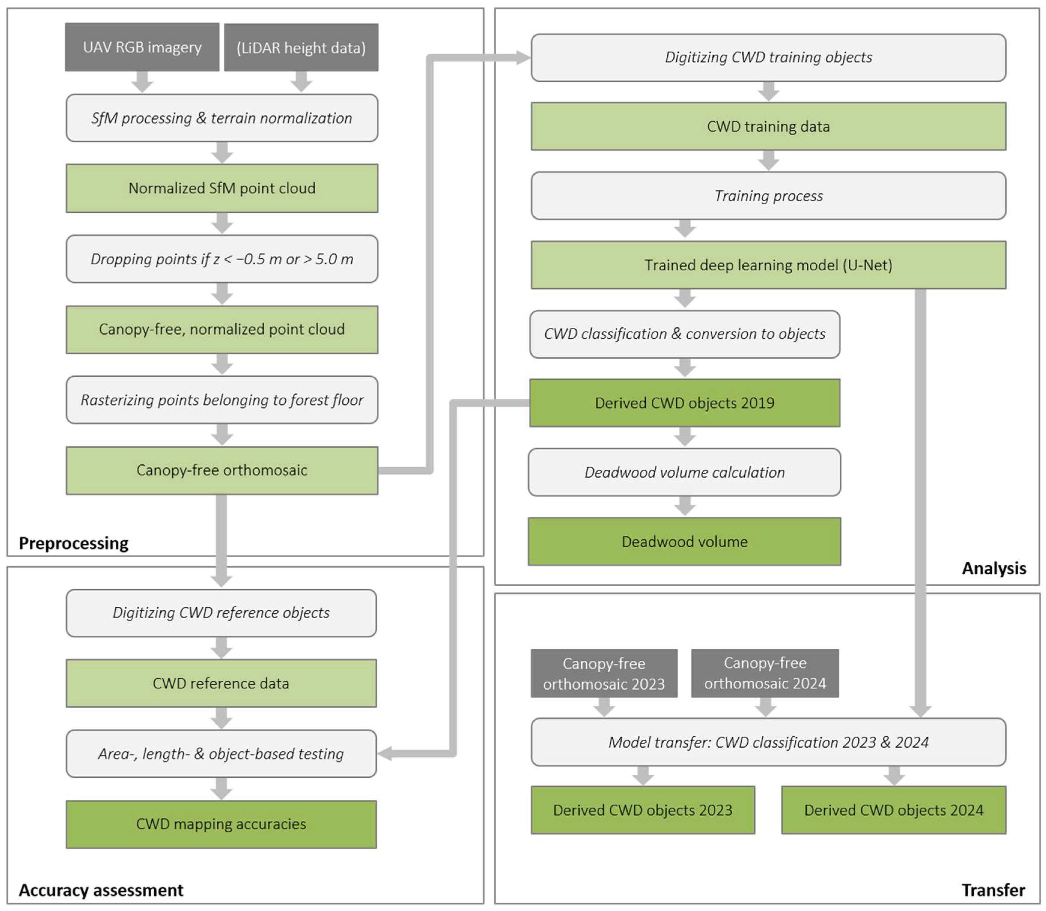
2. Material and Methods
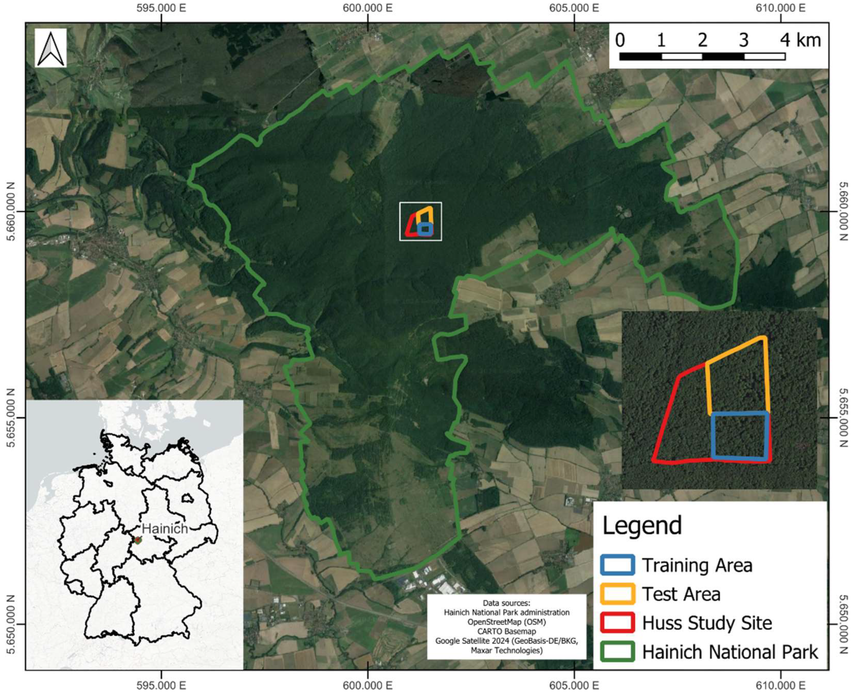
2.1. Study Site

The study site is situated within Hainich National Park, located in the federal state of Thuringia, central Germany (Figure 1). This area, a United Nations Educational, Scientific, and Cultural Organization (UNESCO) World Heritage Site, extends across 75 km2 and plays an important role in the preservation and protection of primeval beech forests in Europe [29]. The altitude ranges from 225 to 494 m above sea level, as it is positioned along a mountain range [30]. Our research focuses on the Huss study site, which comprises 28.2 ha in the core area of the Hainich National Park [31]. The site is characterized by a dense, structurally diverse, multi-layer forest stand, with an average tree cover density of 91% [27]. A 2013 forest inventory of the Huss site conducted by the Hainich National Park administration revealed that European beech (Fagus sylvatica) is the predominant tree species in this area, comprising 78% of the total tree population. However, a wide variety of other tree species are also present, including ash (Fraxinus excelsior), sycamore maple (Acer pseudoplatanus), or hornbeam (Carpinus betulus) [32]. The maximum tree height is approximately 42 m, with an average canopy height of 29 m and a tree density of 725 trees/ha. According to the inventory, the dominant stand (Kraft classes I–III) accounts for 22% of the total number of trees, while the suppressed stand (Kraft classes IV–V) compromises 70% of the trees, with the remaining trees unclassified. This highlights the significant presence of small and understory trees at the study site. The forest also provides a habitat for various fungi and animals, like wildcats, bats, woodpeckers, deer, and many more [33]. Notably, the forest endured significant damage due to unusual droughts in 2018 and 2019, prompting intensified studies on deadwood identification [34]. The coordinates center of the Huss site is at 10°26′5″E and 51°4′47″N. Most of the park, around 90%, is free from current anthropogenic use and not managed.

2.2. UAV Imagery Acquisition

The RGB imagery used for the generation of the orthomosaic was collected with a DJI (Da-Jiang Innovations Science and Technology Co., Ltd., Shenzhen, China) Phantom 4 Pro with a Real Time Kinematic (RTK) global navigation satellite system (GNSS) receiver and camera with a 1″ CMOS sensor, a focal length of 8.8 mm, and a wide-angle field of view of 84°. This feature is highly beneficial when dealing with very high-resolution imagery, as it facilitates direct georeferencing with positioning accuracy in the range of centimeters [35]. Position correction data were supplied by the German Satellite Positioning Service (SAPOS), with the closest reference station approximately 14.5 km away.
To optimize the visualization and coverage of the forest floor, the UAV mission was conducted from the flux tower platform [36] in the leaf-off season of early spring on 24 March 2019. The conditions during the flight were optimal, with wind speed ranging from 0.5 to 1.0 m/s and a fully overcast sky, ensuring consistent illumination and minimizing potential disturbances, such as shadows, in the subsequent image. A parallel flight pattern with a fixed flight height above the starting point, as usually practiced in airborne campaigns, was chosen, and the nadir images were generated with a high overlap percentage of 85% (front) and 80% (side). This high overlap percentage is essential for the generation of the 3D point clouds in the following step. A total of 578 images with a mean ground resolution of 4.18 cm were taken. Given the high precision of the geolocation of the UAV imagery, ground control points were deemed unnecessary, and georeferencing was incorporated in the subsequent processing steps. Previous work shows sufficient geolocation accuracy relying solely on the onboard RTK GNSS signal [37]. Comprehensive details regarding the UAV and camera specifications can be referred to in Thiel et al. [18].
The acquired RGB imagery from the UAV flight mission was processed using a Structure from Motion (SfM) approach previously presented in detail by Thiel et al. [18] using the ETRS89/UTM 32N co-ordinate system (EPSG: 25832). The SfM approach is a stereoscopic photogrammetric method for the derivation of 3D point clouds from multiple 2D images [38]. The principle underlying this method involves utilizing diverse angles of a specific point to determine its 3D spatial coordinates, a process made possible by capturing images with a high percentage of overlap. Subsequently, distinctive features across these multiple images, captured from varying perspectives, are employed to render a 3D object from the original 2D imagery in a stereoscopic way [39]. For the 3D reconstruction process, the software Metashape (Agisoft LLC, St. Petersburg, Russia, version 1.5.1) was employed. An SfM point cloud with an average point density of 1424 pts/m2 was generated. To focus on objects of specific heights, a normalization process was applied by subtracting an airborne LiDAR-based ground elevation dataset from the SfM point cloud, producing height values relative to the ground. The ALS dataset, acquired in 2017, was sourced from the Thuringian State Office of Land Management and Geological Information (geoportal.thueringen.de). Although ground classification could be derived from the leaf-off point cloud itself, the external ALS dataset was used to maintain consistency with Thiel et al. [18] and to allow direct comparison of the two approaches. Differences in ground height between the ALS dataset and internal ground classification were found to be negligible [27]. Using LASTools software (rapidlasso GmbH, Gilching, Germany, version 211112), all points in the point cloud with height values below −0.5 m and above 5.0 m were removed, effectively excluding the canopy from the dataset. This process left only points near the ground and beneath the forest canopy, resulting in a ground-only point cloud with an average density of 864 pts/m2. These points were subsequently rasterized to create a canopy-free orthomosaic.
In order to transfer the trained model to other time steps, two additional leaf-off UAV datasets from 21 March 2023 and 12 March 2024 were obtained from the same study site using a DJI Mavic 3 Enterprise with an RTK module. These datasets underwent the same processing steps as the dataset from 24 March 2019, resulting in a canopy-free orthomosaic. An overview of the flight missions, acquisition parameters for all three UAV datasets, and the resulting SfM processing parameters are provided in Table 1. The datasets from 2023 and 2024 were utilized to apply the trained model, initially developed using the 2019 dataset, to assess the model’s transferability.

2.3. Deep Learning-Based CWD Mapping

An overview of the methodology applied in this study is presented in Figure 2. Generating the training data, training, and classification was performed utilizing ArcGIS Pro (Esri, Redlands, USA, version 2.8.2) and its DL tools from the Image Analyst extension. It was run on an NVIDIA GeForce RTX 3070 Ti 8 GB laptop GPU, Intel i9-12900H CPU, and utilized 32 GB RAM.

2.3.1. Training Data Generation

The process of generating labeled data for the mapping of CWD was undertaken through manual digitization of deadwood polygons on the canopy-free orthomosaic. The area selected for digitization of the training data, hereafter referred to as the “training area”, was located in the southeastern part of the Huss study site (Figure 1). This ensured no interference with reference data generated for the accuracy assessment, situated in the northeastern quadrant (Figure 1).The southeastern part was chosen due to its comparatively higher deadwood density relative to the western part of the study site. The digitized area encompassed a total of 1622.5 m2 of deadwood, spread over an area of 16.3 ha. Subsequently, a labeled train ing dataset was synthesized using the canopy-free orthomosaic and the delineated deadwood polygons from the training area. The image chips were generated with dimensions of 256 × 256 pixels, and a stride of 128 × 128 pixels was applied, resulting in an overlap of 50%. This overlap ensures that each part of the image is seen multiple times in different contexts, with the aim of improving the model’s robustness and reducing edge effects. To further enhance the training dataset and potentially mitigate overfitting, various rotation angles between 10° and 90° were applied during data augmentation. The resulting F1-scores were compared to evaluate performance. The number of image chips varied from 7978 without data rotation to 285,152 with a 10° data rotation. Ultimately, a rotation step of 30° was chosen (95,324 image chips), as this approach represented a compromise: Additional rotations did not yield significant improvements in performance but would have substantially increased both the dataset size and the subsequent training time (Figure 5). Other types of data augmentation, aside from image rotation, were not applied.

2.3.2. Model Training and Classification

U-Net is a CNN architecture designed to capture both local and global contextual information by considering surrounding pixel relationships during the classification process [40]. Its encoder–decoder structure, combined with skip connections, makes it highly proficient in image segmentation tasks. U-Nets are widely recognized for providing pixel-based semantic segmentations and are extensively employed in remote sensing projects. Previous studies have demonstrated the exceptional performance of U-Net approaches in forestry applications [30,41]. Consequently, a U-Net was selected for this study to segment downed deadwood. The model was trained as a U-Net pixel classification model, utilizing a ResNet-34 pretrained on the ImageNet-dataset (www.image-net.org) as a backbone. A ResNet (Residual Network) model is a DL architecture that introduces skip connections or shortcuts between layers helping to train very deep networks more effectively [42]. A pretrained ResNet-50 and ResNet-101 were also tested, but as they did not provide an improvement in accuracy and resulted in a huge increase in training time, the ResNet-34 was chosen. The pre-trained backbone layers were unfrozen so they could be adapted to the existing data. The previously generated training dataset served as an input and was divided into training and validation sets at a ratio of 90% to 10%. Both the training and validation sets were spatially distinct from the area used for the accuracy assessment (test area), with no overlap between them. The maximum training duration was designated as 30 epochs, with an optional early stoppage implemented if the model ceased to improve. A batch size of 8 was chosen and an adaptive moment estimation (Adam) optimizer [43] was used [44]. Since no learning rate was specified, ArcGIS Pro was programmed to automatically infer an optimal learning rate throughout the training process, leading to either an increase or decrease in the learning rate, depending on the gradient. The final learning rate ranged between 1.318 × 10⁻⁵ and 1.318 × 10⁻⁴.
Utilizing the trained U-Net model, the classification of deadwood was carried out on the canopy-free orthomosaic, producing an output raster comprising the classified CWD pixels.

2.3.3. Transferability of the Trained Deep Learning Model

Following the training of the U-Net model on the leaf-off dataset from 2019, the trained DL model was applied on two additional datasets from the same study site. This aimed to assess the transferability of the model to other time steps, and therefore its robustness. The CWD classification involved utilizing the trained model on the canopy-free orthomosaics from 2023 and 2024 without any prior changes to the model architecture or weights.

2.3.4. Calculation of Deadwood Volume

The CWD polygon objects, classified using the DL approach, were utilized to estimate the deadwood volume for all detected objects. To obtain the width of the stems, centerlines were automatically generated for every polygon larger than 0.2 m2 using the QGIS (version 3.34) plugin Geometric attributes [45]. Perpendicular lines to these centerlines were generated, corresponding to the width of the polygon at that specific point. An interval of 20 cm with a starting offset of 10 cm was applied between each measurement. Thus, we divided the stem into slices of 20 cm length and assumed a perfect cylindric form for each of these slices. The volume ( V ) was calculated using the width ( w ) and the interval between every measurement of 20 cm:
V = π × 0.2 × ( 0.5 × w ) 2
Due to the lack of volume in situ reference data, the calculated values from the classified deadwood objects could only be compared to those derived from the reference polygons, using the same methodology for volume calculation.

2.4. Comparative Analysis: Object-Based Image Analysis (OBIA) Approach

We compared the results of the DL model to an OBIA approach developed by Thiel et al. [18]. Their analysis involved a line recognition strategy based on the spectral properties of the canopy-free orthomosaic and was conducted using the software eCognition (Trimble Geospatial, version 9.2).
Given the linear nature of CWD objects, the algorithms first extracted line features from each channel of the RGB image, with parameters such as line length, line width, border width, and line direction fine-tuned for optimal line detection. To ensure lines were identified regardless of their orientation, a loop was designed to encompass angles ranging from 0 to 179°. After line generation, a process of segmentation and classification was implemented, thereby categorizing all objects into line and non-line entities. Objects with an area size less than or equal to 30 pixels were eliminated. Adjacent objects, that indisputably belonged together and were a maximum of two pixels apart, were merged.

2.5. Accuracy Assessment

To assess the accuracy of the OBIA and DL methods and to compare their performance, three distinct methods were employed: area-based, length-based, and object-based testing. These methods were applied to a reference dataset within the test area (Figure 1), which was not used during the training process. The length- and object-based methods were adapted from Thiel et al. [18], as well as the reference dataset, which was created by manually digitizing all CWD objects within the test area.
The area-based assessment method involved comparing the classification results with the reference on a pixel-based level. Overlapping pixels in both layers were marked as true positives (tp), while missed pixels in the classification results were marked as false negatives (fn), and pixels classified as deadwood without a corresponding reference object as false positives (fp). The total area of these categories was then calculated.
The length-based assessment was performed by measuring the length of each CWD object within the canopy-free orthomosaic. To this end, lines were drawn manually along the longest connection of each deadwood object, from the stump to the farthest top branch, following the form of the stem. Deadwood trees with multiple connected branches were represented by a single line, whereas branches separated from the main trunk were given individual lines and treated as separate objects. Only objects with a minimum length of 2 m and a minimum width of 15 cm at their widest point were considered for both the reference and the classified datasets. These values align with the definition of deadwood used by the Hainich National Park administration and were therefore applied accordingly. Line segments were classified as tp when they overlapped with the reference polygons. Fn segments were reference line segments that did not overlap with the classified polygons, and fp segments were classified line segments that did not overlap with the reference polygons. To allow for minor deviations in the position of the central line between the classification approaches and the reference, the reference and classified polygons were buffered 25 cm before being used for the accuracy assessment. The cumulative value for each category was calculated to obtain the accuracy results.
Given the abundance of small branches within the study site, which notably contribute to the total length in each category, the reference and classified line data were filtered additionally for lines with a minimum length of 10 m. The length-based accuracy assessment was then repeated with this filtered dataset.
In the object-based accuracy assessment, any object with over 50% of its length accurately classified was considered a tp object, while overlooked objects were tagged as fn and falsely detected objects as fp. Precision, recall, the relative bias (rBias), and F1-score are then calculated for the area-, length- and object-based methods.
These three accuracy assessments were applied to both the OBIA and the DL classification results. To ensure consistency, all manual digitization tasks were performed by the same person. This approach aimed to apply the same criteria across all datasets, acknowledging that manual digitization is inherently subjective, especially in cases where the presence of a CWD object cannot be clearly determined from either the height data or the orthomosaic. Consequently, the accuracy assessment for the OBIA results were completely reperformed, rather than relying on the results from Thiel et al. [18]. This was performed to ensure the same methodology for both methods and therefore maintain their comparability. We opted for an accuracy assessment using manual digitization instead of in situ data, as our study involves detailed delineation of deadwood, capturing individual forms of logs and branches. In this case, we are not merely assessing the presence or absence of deadwood but also verifying the delineated shapes and dimensions. Currently, there is no reliable method to obtain high-accuracy field data of such detailed deadwood forms, particularly beneath dense forest canopies and considering the high density of deadwood objects. The primary obstacles include limited RTK correction signals under dense canopy cover (even during leaf-off season signal availability is restricted to canopy gaps), complicating accurate differential GNSS-based georeferencing. This is in line with the majority of remote sensing studies on downed deadwood mapping using manually delineated reference data [23,24,26,46,47,48]. To account for possible subjectivity introduced in the reference process, we included a robust testing dataset including 1110 reference objects, totaling 7459.67 m of deadwood.

3. Results

This section focuses on the performance metrics of the DL classification, the influence of DL model parameters (rotation angle for training data augmentation), the comparative analysis results between DL and OBIA approaches, and the model’s transferability to other years.

3.1. Deep Learning-Based Classification Results

The optimal model utilized a U-Net structure with a ResNet-34 backbone. Implementing 30° rotation data augmentation, the model achieved precision, recall, and F1-score values of 0.794, 0.704, and 0.746, respectively. Some exemplary subsets of the classification results are shown in Figure 3. The total volume of all CWD objects within the study site summed up to 2128.05 m3. Considering only the CWD objects within the test area, the volume derived from the classification results totaled 1051.80 m3, while the volume based on the reference CWD objects was 1202.03 m3. Thus, the calculated volume underestimates the reference volume by 150.94 m3 or 12.48%.

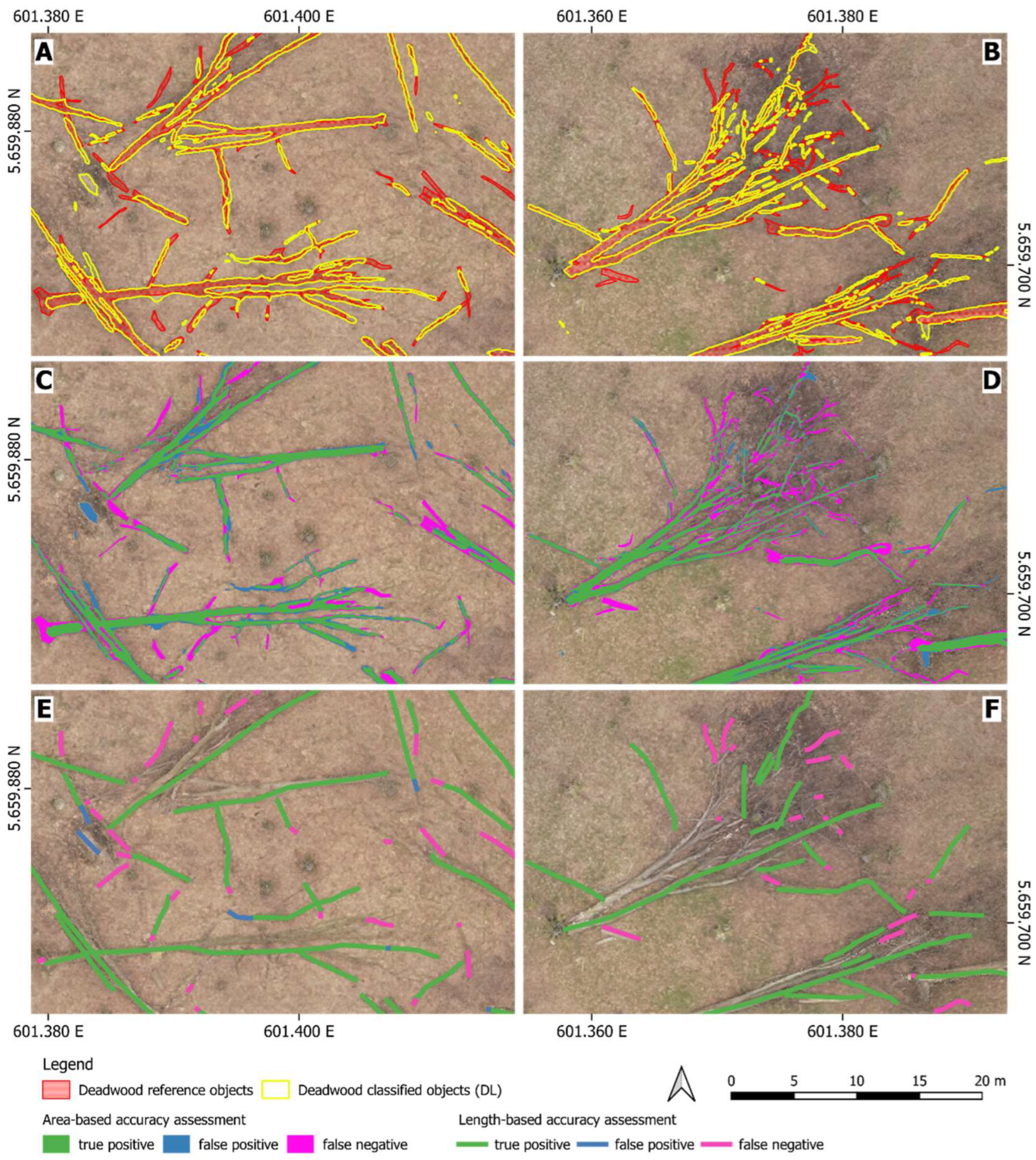
3.1.1. Area-Based Accuracy Assessment

Figure 4 illustrates two subsets of the area-based assessment, displaying the corresponding tp, fn, and fp areas. The model demonstrates a strong ability to accurately distinguish between deadwood and forest floor, particularly for bigger CWD objects. Overall, the area-based accuracy assessment yielded a precision of 78.5% and a recall of 67.6%, resulting in an F1-score of 72.6% (Table 2); thus, omitted deadwood areas predominate over erroneously detected areas, indicated also by the negative bias value. Particularly, smaller branches, which, due to their abundance in the study site, contribute notably to the total area, were not always detected by the model. Also, the bigger base parts of a stem tend to be an area for confusion. Notably, there was no observed bias in the width of the objects, resulting in a realistic stem form that corresponds well with the stem form present in the orthomosaic. In fact, the classified stem form in some parts seems to be more precise and realistic than that found in the reference dataset.

3.1.2. Length-Based Accuracy Assessment

The results for the length-based assessment show a similar trend to those of the area-based one (Figure 4 and Table 2), although the accuracy measures are approximately 15% higher. The length of all deadwood objects larger than 2 m and wider than 15 cm summed up to 7459.67 m for the reference dataset and 5662.72 m for the DL-classified dataset. The high precision value of around 97% indicates the reliability of the detected CWD lengths.
Additionally, accuracy measures only for longer stems (>10 m) were calculated (Table 2). The F1-score improved by around 8% to a value of 96% when only deadwood longer than 10 m was considered, underscoring that a notable part of the missed lengths corresponds to smaller branches (<10 m), and a minor part to slight differences in the exact length of bigger stems.

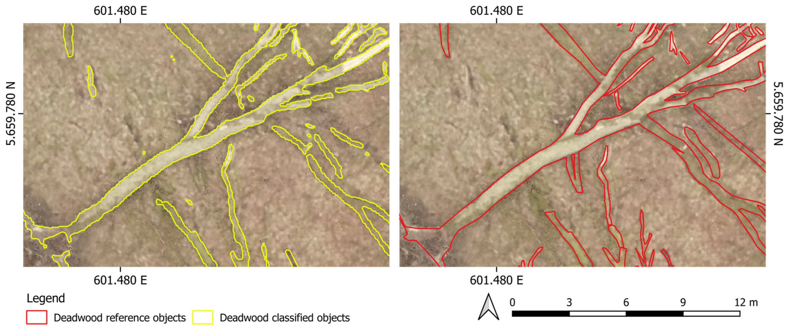
3.1.3. Object-Based Accuracy Assessment

As a result of the line digitization of deadwood objects within the reference dataset, a total of 1110 CWD objects were identified. In comparison, within the results provided by the DL model, 721 CWD objects were annotated. Among these, a vast majority (700 out of 721) were accurate. However, 268 objects from the reference dataset were missed out by more than 50% and therefore classified as missing. Consequently, the results yielded a recall of 72.31% and a precision of 97.09% (Table 2).

3.2. Impact of Deep Learning Model Parameters on CWD Detection

As depicted in Figure 5, each halving of the rotation angle corresponds to a doubling in the number of training images, resulting in an approximately doubled training duration. The lowest accuracy was observed with non-augmented data, but even smaller rotation angles of 90° and 60° exhibited substantial performance improvement. While there was a general tendency of better F1-scores with larger training datasets, the increments in performance tended to be considerably smaller than the corresponding increase in training time. Some data augmentation steps even led to slightly lower accuracy compared to the preceding step. The best results, with an F1-score of 0.782, were obtained using the smallest tested rotation angle (10°); however, a rotation angle of 30° (second best F1-score) was ultimately chosen due to the large differences in training time.

3.3. Comparative Analysis: Deep Learning vs. OBIA Classification Performance

The comparison of the accuracy assessment results of both methods demonstrates that the DL approach outperforms the OBIA methodology (Table 2), as accuracy measurement for all three methods resulted in higher values for the DL classification.

3.4. Model Transferability for Deadwood Detection in 2023 and 2024

The trained model was successfully applied to the canopy-free orthomosaics of 2023 and 2024 and CWD objects were classified (Figure 6). Since no reference data were available for those years, the accuracy assessment was conducted solely on a qualitative basis. The classified deadwood areas were visually observed and appeared to be highly reliable. As shown in Figure 6, some of the deadwood objects from 2019 decomposed, reducing in size or turning completely into humus, which was correctly detected by the model. However, the number of missed out areas, lengths, and entire objects is substantially higher for the classification results of 2023 and 2024 compared to those from 2019.

4. Discussion

4.1. Performance of the DL-Based CWD Mapping

The accuracy measures of the three performed assessment methods demonstrate the high suitability of the applied DL approach for detecting deadwood. The reliability of the detected area and length is very high, as indicated by high precision values. There are rarely any cases where other objects on the forest floors or data noise in areas with missing ground information were mistakenly identified as deadwood. However, the lower recall values and a negative bias reflect that some deadwood objects or parts of them were missed.
To our knowledge, the number of comparable studies that employ UAV data for log detection remains quite low. Remote sensing-based analysis tends to focus on the detection of snags or the use of ALS to detect logs. We compared the accuracy values of this study (F1-score between 73% and 96%) to those of similar studies. Panagiotidis et al. [23] obtained a Kappa index of 0.44, Inoue et al. [20] achieved an 80–90% detection rate for logs, Bulatov and Leidinger [26] classified snags and logs together, achieving an overall accuracy of 92% and a mean average precision of 43%, and Jiang et al. [24] reported a recall of 68% and a precision of 99% for log detection—all of them by using high-resolution UAV or airborne data. However, due to the variety of accuracy methods and metrics applied, as well as the diversity of different forest ecosystems and canopy densities, it is difficult to compare the values solely quantitatively. We applied three different accuracy assessments, each focusing on slightly different aspects (area vs. length vs. objects). Although the tendencies, such as higher precision than recall values, remained consistent—similarly to the findings of Jiang et al. [24] for logs and Tao et al. [49] for snags—the values spanned a wide range of around 20 percentage points. Therefore, we recommend considering the type of accuracy assessment when comparing results and including a clear description of the test methods applied.
Comparing the accuracy measures with CWD objects of a minimum length of 10 m revealed that many of the missed parts are small branches, typically only a few meters in length. These branches are abundant in the Huss study site, where mostly wind-thrown, dried trees tend to shatter and break when they fall. Many of these branches overlap, further complicating their detection. These challenges of detecting smaller branches were also reported by Inoue et al. [20], reporting difficulties in detecting logs shorter than 10 m. Another challenge is detecting highly decomposed CWD objects. As decomposition progresses, it becomes harder to distinguish these objects visually from the ground, because they gradually blend into it, making it difficult to draw a clear boundary as the CWD objects slowly disappear over time. However, for estimations of biomass and carbon storage, these challenges may not be of major concern, as small branches or decomposed stems account for less biomass and carbon than the larger and intact ones [50].
One essential factor in remote sensing-based analysis is the acquisition of reference data that accurately represents reality. This is especially important for DL approaches, where the amount and quality of training data are important. Given that UAV data provides resolutions and positional accuracies within a few centimeters, the need for equally precise reference data for accuracy assessment purposes increases. In this study, manually generated data based on visual interpretation of the UAV data products were used. While this approach is not ideal, it is often the only feasible option due to the challenges of obtaining georeferenced data with centimeter-level positional accuracy under dense canopies. Nevertheless, the manual nature of this task is always subject to some degree of subjectivity and varying interpretations. In some instances, interpreting the available UAV data products to determine the presence of deadwood was difficult, particularly for small and decomposed objects. This created situations where based solely on the available UAV-SfM data, it is difficult to determine whether the classified CWD objects or reference data provide a more accurate picture. Although several objects were still omitted, in some areas, the classification appeared visually with a higher degree of detail than the actual reference objects, as illustrated in the subset in Figure 7.
Since manual digitization is also a time-consuming task, the amount of reference data for training is limited. Therefore, it was artificially enhanced by rotating the input images. Data augmentation in DL is widely applied and recommended to improve accuracies, robustness, and to prevent overfitting [51,52,53,54,55]. In this study, data augmentation improved the accuracy values, although the sharp increase in training time did not go along with a substantial increase in accuracy (Figure 5).

4.2. Comparative Analysis Between the DL and OBIA Approach

The comparison of the three methods for accuracy assessment clearly demonstrated that the U-Net classification delivered better results concerning the correct area, length and objects, compared to the OBIA classification. All F1-scores show a significant margin between the DL and OBIA results of at least 15 percentage points. Especially, the form and width of the detected deadwood are far more precise and detailed within the DL classification; this is represented in the comparable low precision values for the OBIA area assessment, reflecting an overestimation in width and the difficulty to delineate single branches with a line detection approach. This result is not surprising, as several studies have shown the great potential of recent DL architectures, like U-Nets, for forestry analysis with very high-resolution images [41,56,57]. One advantage of DL methods over traditional approaches lies in their ability to distinguish spectrally similar objects, such as deadwood and the forest floor, by autonomously extracting patterns and considering context information through the generation of feature maps during the training process. Traditional methods, in contrast, require a manual selection of a set of features, like indices, filters, or texture metrices [58]. While DL is already well established for remote sensing-based forestry applications, direct comparisons between traditional and DL methods using the same input data and test parameters can help in understanding the advantages and limitations of each approach. Such comparisons should also include assessing the generalization ability of DL models, which often still lag behind traditional methods when applied to different datasets.

4.3. Generalization of the DL Model

For practical application in the field of forestry, it is crucial to develop models not only suitable for one dataset, but usable for different forest sites, UAV sensor types, image parameters, and acquisition times. This challenge was addressed by applying the trained model to two other datasets from different years and different sensor types, although the study site remained the same. The classification results demonstrate that the model’s general application to other time steps is feasible and produces reliable classified deadwood objects. However, the higher rate of omitted deadwood objects needs to be highlighted and improved. A possible explanation is that the model may have overfitted to the 2019 dataset, limiting its ability to detect slightly altered deadwood features in later datasets, leading to omissions. This could be due to differences in lighting conditions and the use of different UAV sensors, each with unique camera characteristics. These factors influence image contrast and cause variations in the RGB histograms, which may affect the model’s ability to generalize across datasets.
Further steps could include applying additional forms of data augmentations to those already employed in this study [59], or incorporating more diverse training data from other time steps. Additionally, further generalization efforts should involve applying the model to different deciduous forest study sites.
However, in the field of forest remote sensing, labeled data remains scarce for most applications. For DL studies, the most time-consuming aspect is typically generating sufficient training data, often through manual labeling, and the training process itself. Obtaining a large volume of labeled training data that covers different scenes, which is necessary for creating generalized models, is often unfeasible. This makes it challenging to apply DL to diverse forest sites and forest ecosystems. To overcome these limitations, valuable community-driven and open-source data collection efforts already exist for some forest parameters, creating benchmark training datasets for forestry applications. Examples include the deadtrees.earth project [60] for standing deadwood and BAMFORESTS [61] for individual tree crown delineations.
Generalization approaches from computer vision, such as transfer learning, domain adaptation [62], or domain generalization [63], are beginning to be applied to remote sensing [64] and could offer solutions to this issue. Transfer learning, especially using pretrained models typically trained on the ImageNet dataset, has become common practice in classification tasks [65]. In this study, a pretrained ResNet-34 was used; although deeper models such as ResNet-50 and ResNet-101 were tested, they did not notably improve performance while increasing training time. Additional methods to address the domain shift problem when applying the model to different time steps were not explored in this study but are worth considering for future research.

4.4. Use of Deadwood Detection Results for Further Forest Analysis

The derived deadwood using the proposed method can be considered as a first step for further forest analysis within different forest monitoring and management contexts. Accurate mapping of CWD can be utilized for various ecological and climate studies, as well as forest management plans. Therefore, improvements in accuracy of deadwood mapping approaches, such as the one presented here, provide valuable data and information for the forestry sector. Examples of the use of deadwood mapping include its role as a proxy for biodiversity [8], its impact on recreational activities [66], its contribution to the carbon cycle [67], and its role in forest restoration [68].
To be utilized for these analyses, it may be necessary to generate processed forest parameters from the deadwood mapping information. Several studies have developed methods to derive CWD volume, e.g., from airborne LiDAR deadwood mapping [69,70] and optical airborne data [21]. We used the classified CWD objects to calculate deadwood volume for the entire study site by applying a straightforward approach of fitting cylindric slices into the stems. The comparison between volume derived from classified and reference polygons yielded similar results. The slight underestimation in the calculated volume reflects the classification’s tendency to omit CWD parts, as indicated by the false negative rates in the area-, length-, and object-based assessments. While this approach might deliver promising results, it is important to acknowledge that, since the comparison relies on the same methodology lacking in situ volume reference data, it does not constitute an independent accuracy assessment.

5. Conclusions

This study successfully developed a DL approach for detecting CWD in a structurally diverse and dense deciduous forest environment. The canopy-free orthomosaics generated via SfM from very high-resolution UAV data resulted in an excellent data product for deadwood mapping with DL. By implementing a U-Net architecture with a ResNet-34 backbone and utilizing data augmentation techniques, the model achieved very high classification performance, with F1-scores between 72.62% and 95.97%. Delineation of CWD objects from the underlying ground and representing a precise stem form was achieved with a high level of detail, despite the spectral similarity between deadwood and ground. Very high precision values (78.49–98.96%) highlight the reliability of the mapping results, while recall values have lower ranges (67.57–93.15%), demonstrating that CWD objects were missed out and could not be detected. The model results were assessed for the CWD of different minimum lengths, showing that the accuracy values rise when considering only larger objects, thus leading to a higher rate of omission for smaller objects.
The results from the DL approach were compared to the traditional OBIA approach implemented by Thiel et al. [18] by applying the same accuracy assessment steps to both results. The DL model demonstrated higher precision, recall, and F1-scores across various assessment methods of at least 15 percentage points compared to the OBIA approach and clearly outperformed the traditional mapping technique.
The study also highlighted the challenges and importance of generalizing the DL model across different datasets and time steps. While the model showed promising results when applied to other datasets from different years and sensor types, it exhibited a higher rate of omitted deadwood objects. Future work should focus on incorporating more diverse training data and exploring advanced generalization techniques, such as transfer learning and domain adaptation, to improve the model’s applicability to various forest sites and conditions.
The findings emphasize the potential of DL methods in forestry applications, particularly in enhancing the accuracy and detail of deadwood detection. Accurate mapping of CWD is important for ecological studies, forest management, and conservation efforts. The derived deadwood data can serve as a valuable resource for further forest analysis, contributing to biodiversity monitoring, carbon cycling assessments, and forest restoration initiatives.
In conclusion, this study demonstrates the feasibility and advantages of using DL approaches for deadwood detection with very high-resolution optical UAV data, paving the way for more sophisticated and generalized models in the future. Continued advancements in DL techniques and increased availability of labeled training data will further enhance the capabilities and applications of such models in forestry and environmental research.

Author Contributions

Conceptualization, C.T., B.S. and S.D.; methodology, S.D., B.S. and M.M.M.; software, B.S. and S.D.; validation, H.A., S.D. and M.M.M.; formal analysis, S.D., M.M.M. and B.S.; investigation, S.D., M.M.M., H.A., B.S., C.D., M.A. and C.T.; resources, S.D., C.D. and C.T.; data curation, S.D., S.H. and B.S.; writing—original draft preparation, S.D., B.S. and M.M.M.; writing—review and editing, S.D., M.M.M., C.D., S.H., M.A., H.M. and C.T.; visualization, S.D. and M.A.; supervision, C.T., H.M. and C.D.; project administration, C.T., C.D. and S.D.; funding acquisition, C.T., C.D. and S.D. All authors have read and agreed to the published version of the manuscript.

Funding

This research received no external funding.

Data Availability Statement

The data presented in this study are available on request from the corresponding author. The data are not publicly available due to privacy reasons.

Acknowledgments

The authors gratefully acknowledge the Hainich National Park administration for their support during the fieldwork. We also extend our sincere thanks to the University of Göttingen for granting us access to the flux tower platform, which was essential for the successful launch and landing of the UAV.

Conflicts of Interest

The authors declare no conflicts of interest.

Appendix A

Table A1. Literature overview of ALS, TLS, and image-based deadwood mapping approaches. Abbreviations: DEM = digital elevation model, nRMSE = normalized root mean square error, CIR = color-infrared, R-CNN = region-based CNN.
PaperSensor, PlatformMethodResolutionResearch AreaDeadwood
Type
Results
[69]ALSRegression models4 pts/m2,
DEM 1 m res.
(area-based)
Koli National Park—eastern FinlandLogs and
snags
nRMSE of the volume prediction: 51.6% (downed), 78.8% (standing), and 12.7% (living trees)
[71]ALSProbability proportional to size sampling and probability layers derived from LiDAR data0.5 pts/m2
(area-based)
Central Finland, 305.8 haLogs and
snags
Auxiliary laser data can increase CWD detection accuracies
[72]ALSRandom Forest to predict dead basal areaN/A
(area-based)
Bark beetle affected areas in the USASnagsIntensity metrics were important in predicting dead basal area
[70]ALSRegression models with discrete-return and full-waveform LiDAR, leaf-on and leaf-off combined5.0 pts/m2 (leaf-on) and 5.2 pts/m2 (leaf-off)
(area-based)
New Forest National Park, southern England, 2200 haLogs and
snags
nRMSE of the volume prediction: 16% (standing), 27% (downed)
[19]ALSBi-temporal LiDAR data, allometric equations>20 pts/m2, Canopy Height Model 0.5 m res.Helsinki National Park, 14.9 haLogs97.8% new downed trees, 89% species group prediction
[46]ALSRule-based OBIA≥9 pts/m2Near Last Chance in Placer County, CA, USA, 11 haLogs73% identified logs
[47]ALSDEM based on multi-temporal, full waveform LiDAR, map algebra22–40 pts/m2 (leaf-on), 17–20 pts/m2 (leaf-off), Beech forest, Uckermark, Germany, 110 ha, and Lägern, Switzerland, 9 haLogs and
snags
70.5% identified logs (37.3% fully, 33.2% partially)
[73]ALSLine template-matching69 pts/m2Managed hemi-boreal forest southwest of Sweden, 54 haLogs41% stem matching
[74]ALSNormalized cut algorithm30 pts/m2 (leaf-off)Bavarian Forest National Park, GermanyLogs90% fallen stems while having 30–40% overstory presence with a precision of 80%
[48]TLSCylindrical shape detection and mergingHigh point densityBavarian Forest National Park, GermanyLogsDowned trunks completeness up to 0.79
[75]TLSCylinder fittingHigh point densityEvo, southern FinlandLogsDowned trunks completeness of 33% and correctness of 76%
[76]ALS, UAV LiDAR, TLSClustering based on geometrical (planarity) and intensity point cloud features171–7457 pts/m2
(leaf-off)
Plantation and natural forest, USALogsAverage recall of 0.83 and precision between 0.40 and 0.85
[77]CIR image, airborneManual digitization on imagery using GIS23 cm res.Spruce forests, SwitzerlandSnags82% of intact snags, 67% broken snags detected
[78]RGB image,
UAV
Classifications: Pixel-based (decision trees) and object-oriented 6.8–21.8 cm res.Riparian forest, France, 174 haSnagsObject-oriented: 80% with respect to omission errors and 65% with respect to commission errors
[22]CIR image, airborneHybrid classification (e.g., ISODATA clustering, OBIA), regression model (area-based)25 cm res.Gatineau Park, CanadaSnags,
logs volume
Snags: accuracy of 94%, regression models with high errors
[79]CIR image + ALSSingle-tree classification using logistic regresion17 cm and 9.5 cm res., LiDAR: 55 pts/m2Šumava and Bavarian Forest National Park, 924 km2SnagsOverall accuracy of 82.8–92.6%
[21]RGB image, airborneTemplate matching, machine learning approaches for volume prediction0.2 m res.Tuscany Region, Italy, 456 km2LogsR2 = 0.92 with SVM regression for volume prediction of windthrown trees
[20]RGB image,
UAV
Manual detection0.5–1 m res.Ogawa Forest Reserve in Kitaibaraki, Japan, 6 haLogsInsufficient detection of small CWD, 80–90% accuracy on bigger CWD
[23]RGB image,
UAV
Line template matching 2.68 cm res.West Bohemia, Czech RepublicLogsKappa of 0.44
[80]RGB image,
airborne
Random forest classification, filters0.5 m res.
DEM 1 m res.
Black Forest, Germany, 600 haSnagsUser’s accuracy of 0.74, producer’s accuracy of 0.80 after application of filters
[81]CIR image, airborneClassification using extended VGG-16 (CNN)20 cm res.Province of Quebec, Canada, 32 km2Snags (live vs. dead)Tree health status prediction accuracy 94%
[82]RGB image,
UAV
Object detection using a new CNN5–10 cm res.Nature reserve “Stolby” in Krasnoyarsk, RussiaSnags (damage categories)F-Score up to 88.89% with data augmentation for deadwood classification
[30]RGB image,
UAV
Semantic segmentation using adapted U-Net<2 cm res.Hainich National Park and Black Forest, Germany, 51 haSnags (deadwood and tree species)Mean F1-score of 73% classifying several tree species including deadwood
[83]RGB image,
UAV
Segmentation using YOLOv8x-seg25 cm res.Júcar river, SpainWood debris in riverAccuracy strongly depends on the characteristics of the debris
[24]CIR image, airborneSemantic segmentation using optimized FCN-DenseNet10 cm res.Bavarian national forest park, GermanyLogs and
snags
Recall of 94.6% (standing) and 67.8% (downed), precision of 100% (standing) and 99.0% (downed)
[49]RGB image,
UAV
Classification using AlexNet and GoogLeNet (CNNs)8.47 cm res.Jinjiang, Fujiang province in southeastern China, 4.25 km2Snags (dead pine trees)AlexNet: 90% precision, 70% recall, GoogLeNet: 98% precision, 51% recall of dead pine trees
[84]RGB image,
UAV
Object detection using optimized Faster R-CNN N/AJi’an, Jiangxi Province, China, 1.8 km2Snags (pine wilt diseased)Accuracy of 89.1%
[25]RGB image,
UAV
Semantic segmentation using U-Net and heuristic stem reconstruction model<2 cm res.Coniferous forests, GermanyLogsRates of at least 50% stem detection betweem 60% and 96%
[26]RGB image,
UAV
Instance segmentation using Mask R-CNNN/AGerman forestsLogs and snags92.4% overall accuracy, 43.4% mean average precision
[18]RGB image,
UAV
Rule-based OBIA5 cm res.Hainich National Park, 28.2 haLogs83.5% precision, 69.2% recall (length-based)

References

  1. Gardner, C.J.; Bicknell, J.E.; Baldwin-Cantello, W.; Struebig, M.J.; Davies, Z.G. Quantifying the impacts of defaunation on natural forest regeneration in a global meta-analysis. Nat. Commun. 2019, 10, 4590. [Google Scholar] [CrossRef] [PubMed]
  2. van Tiel, N.; Fopp, F.; Brun, P.; van den Hoogen, J.; Karger, D.N.; Casadei, C.M.; Lyu, L.; Tuia, D.; Zimmermann, N.E.; Crowther, T.W.; et al. Regional uniqueness of tree species composition and response to forest loss and climate change. Nat. Commun. 2024, 15, 4375. [Google Scholar] [CrossRef]
  3. Cook-Patton, S.C.; Leavitt, S.M.; Gibbs, D.; Harris, N.L.; Lister, K.; Anderson-Teixeira, K.J.; Briggs, R.D.; Chazdon, R.L.; Crowther, T.W.; Ellis, P.W.; et al. Mapping carbon accumulation potential from global natural forest regrowth. Nature 2020, 585, 545–550. [Google Scholar] [CrossRef]
  4. Winkel, G.; Lovrić, M.; Muys, B.; Katila, P.; Lundhede, T.; Pecurul, M.; Pettenella, D.; Pipart, N.; Plieninger, T.; Prokofieva, I.; et al. Governing Europe’s forests for multiple ecosystem services: Opportunities, challenges, and policy options. For. Policy Econ. 2022, 145, 102849. [Google Scholar] [CrossRef]
  5. Crecente-Campo, F.; Pasalodos-Tato, M.; Alberdi, I.; Hernández, L.; Ibañez, J.J.; Cañellas, I. Assessing and modelling the status and dynamics of deadwood through national forest inventory data in Spain. For. Ecol. Manag. 2016, 360, 297–310. [Google Scholar] [CrossRef]
  6. Harmon, M.E.; Franklin, J.F.; Swanson, F.J.; Sollins, P.; Gregory, S.V.; Lattin, J.D.; Anderson, N.H.; Cline, S.P.; Aumen, N.G.; Sedell, J.R.; et al. Ecology of Coarse Woody Debris in Temperate Ecosystems. Adv. Ecol. Res. 2004, 34, 59–234. [Google Scholar] [CrossRef]
  7. Ravindranath, N.H.; Ostwald, M. Carbon Inventory Methods: A Handbook for Greenhouse Gas Inventory, Carbon Mitigation and Roundwood Production Projects; Advances in Global Change Research; Springer: Berlin/Heidelberg, Germany, 2008; pp. 217–235. [Google Scholar]
  8. Lassauce, A.; Paillet, Y.; Jactel, H.; Bouget, C. Deadwood as a surrogate for forest biodiversity: Meta-analysis of correlations between deadwood volume and species richness of saproxylic organisms. Ecol. Indic. 2011, 11, 1027–1039. [Google Scholar] [CrossRef]
  9. Augustynczik, A.L.D.; Gusti, M.; Di Fulvio, F.; Lauri, P.; Forsell, N.; Havlík, P. Modelling the effects of climate and management on the distribution of deadwood in European forests. J. Environ. Manag. 2024, 354, 120382. [Google Scholar] [CrossRef] [PubMed]
  10. Nyström, M.; Holmgren, J.; Fransson, J.E.S.; Olsson, H. Detection of windthrown trees using airborne laser scanning. Int. J. Appl. Earth Obs. Geoinf. 2014, 30, 21–29. [Google Scholar] [CrossRef]
  11. Trumbore, S.; Brando, P.; Hartmann, H. Forest health and global change. Science 2015, 349, 814–818. [Google Scholar] [CrossRef]
  12. European Parliament and Council. Regulation (EU) 2024/1991 of the European Parliament and of the Council of 24 June 2024 on Nature Restoration and Amending Regulation (EU) 2022/869. Official Journal of the European Union. 2024. Available online: https://eur-lex.europa.eu/eli/reg/2024/1991/oj/eng (accessed on 1 April 2025).
  13. Larjavaara, M.; Brotons, L.; Corticeiro, S.; Espelta, J.M.; Gazzard, R.; Leverkus, A.; Lovrić, N.; Maia, P.; Sanders, T.G.M.; Svoboda, M.; et al. Deadwood and Fire Risk in Europe: Knowledge Synthesis for Policy; Publications Office of the European Union: Luxembourg, 2023; Available online: https://www.openagrar.de/receive/openagrar_mods_00090284 (accessed on 1 April 2025).
  14. Schwill, S.; Schleyer, E.; Planek, J. Handbuch Waldmonitoring für Flächen des Nationalen Naturerbes. 2016. Available online: https://www.naturschutzflaechen.de/fileadmin/Medien/Downloads/NNE_Infoportal/Monitoring/Handbuch_Waldmonitoring.pdf (accessed on 1 April 2025).
  15. Maltamo, M.; Kallio, E.; Bollandsås, O.M.; Næsset, E.; Gobakken, T.; Pesonen, A. Assessing Dead Wood by Airborne Laser Scanning. In Forestry Applications of Airborne Laser Scanning; Maltamo, M., Næsset, E., Vauhkonen, J., Eds.; Springer: Dordrecht, The Netherlands, 2014; pp. 375–395. ISBN 978-94-017-8663-8. [Google Scholar]
  16. Marchi, N.; Pirotti, F.; Lingua, E. Airborne and terrestrial laser scanning data for the assessment of standing and lying deadwood: Current situation and new perspectives. Remote Sens. 2018, 10, 1356. [Google Scholar] [CrossRef]
  17. Pignatti, G.; Natale, F.D.; Gasparini, P.; Paletto, A. Deadwood in Italian forests according to National Forest Inventory results. For. Riv. Selvic. Ecol. For. 2009, 6, 365–375. [Google Scholar] [CrossRef]
  18. Thiel, C.; Mueller, M.M.; Epple, L.; Thau, C.; Hese, S.; Voltersen, M.; Henkel, A. UAS Imagery-Based Mapping of Coarse Wood Debris in a Natural Deciduous Forest in Central Germany (Hainich National Park). Remote Sens. 2020, 12, 3293. [Google Scholar] [CrossRef]
  19. Tanhuanpää, T.; Kankare, V.; Vastaranta, M.; Saarinen, N.; Holopainen, M. Monitoring downed coarse woody debris through appearance of canopy gaps in urban boreal forests with bitemporal ALS data. Urban For. Urban Green. 2015, 14, 835–843. [Google Scholar] [CrossRef]
  20. Inoue, T.; Nagai, S.; Yamashita, S.; Fadaei, H.; Ishii, R.; Okabe, K.; Taki, H.; Honda, Y.; Kajiwara, K.; Suzuki, R. Unmanned aerial survey of fallen trees in a deciduous broadleaved forest in eastern Japan. PLoS ONE 2014, 9, e109881. [Google Scholar] [CrossRef]
  21. Pirotti, F.; Travaglini, D.; Giannetti, F.; Kutchartt, E.; Bottalico, F.; Chirici, G. Kernel feature cross-correlation for unsupervised quantification of damage from windthrow in forests. Int. Arch. Photogramm. Remote Sens. Spat. Inf. Sci. ISPRS Arch. 2016, 41, 17–22. [Google Scholar] [CrossRef]
  22. Pasher, J.; King, D.J. Mapping dead wood distribution in a temperate hardwood forest using high resolution airborne imagery. For. Ecol. Manag. 2009, 258, 1536–1548. [Google Scholar] [CrossRef]
  23. Panagiotidis, D.; Abdollahnejad, A.; Surový, P.; Kuželka, K. Detection of fallen logs from high-resolution UAV images. N. Z. J. For. 2019, 49, 1–11. [Google Scholar] [CrossRef]
  24. Jiang, S.; Yao, W.; Heurich, M. Dead wood detection based on semantic segmentation of VHR aerial CIR imagery using optimized FCN-Densenet. Int. Arch. Photogramm. Remote Sens. Spat. Inf. Sci. ISPRS Arch. 2019, 42, 127–133. [Google Scholar] [CrossRef]
  25. Reder, S.; Kruse, M.; Miranda, L.; Voss, N.; Mund, J.-P. Unveiling wind-thrown trees: Detection and quantification of wind-thrown tree stems on UAV-orthomosaics based on UNet and a heuristic stem reconstruction. For. Ecol. Manag. 2025, 578, 122411. [Google Scholar] [CrossRef]
  26. Bulatov, D.; Leidinger, F. Instance segmentation of deadwood objects in combined optical and elevation data using convolutional neural networks. In Proceedings Volume 11863, Earth Resources and Environmental Remote Sensing/GIS Applications XII; Schulz, K., Ed.; SPIE: Bellingham, WA, USA, 2021; p. 37. ISBN 9781510645707. [Google Scholar]
  27. Dietenberger, S.; Mueller, M.M.; Bachmann, F.; Nestler, M.; Ziemer, J.; Metz, F.; Heidenreich, M.G.; Koebsch, F.; Hese, S.; Dubois, C.; et al. Tree Stem Detection and Crown Delineation in a Structurally Diverse Deciduous Forest Combining Leaf-On and Leaf-Off UAV-SfM Data. Remote Sens. 2023, 15, 4366. [Google Scholar] [CrossRef]
  28. Mueller, M.M.; Dietenberger, S.; Nestler, M.; Hese, S.; Ziemer, J.; Bachmann, F.; Leiber, J.; Dubois, C.; Thiel, C. Novel UAV Flight Designs for Accuracy Optimization of Structure from Motion Data Products. Remote Sens. 2023, 15, 4308. [Google Scholar] [CrossRef]
  29. Biehl, R. Der Nationalpark Hainich—“Urwald mitten in Deutschland”. In Exkursionsführer zur Tagung der AG Forstliche Standorts-und Vegetationskunde vom 18. bis 21. Mai 2005 in Thüringen; Wald, T.L., Fischerei, J., Eds.; Thüringer Landesanstalt für Wald, Jagd und Fischerei: Gotha, Germany, 2005; pp. 44–47. [Google Scholar]
  30. Schiefer, F.; Kattenborn, T.; Frick, A.; Frey, J.; Schall, P.; Koch, B.; Schmidtlein, S. Mapping forest tree species in high resolution UAV-based RGB-imagery by means of convolutional neural networks. ISPRS J. Photogramm. Remote Sens. 2020, 170, 205–215. [Google Scholar] [CrossRef]
  31. Huss, J.; Butler-Manning, D. Entwicklungsdynamik eines buchendominierten “Naturwald”-Dauerbeobachtungsbestands auf Kalk im Nationalpark Hainich/Thüringen. Wald. Online 2006, 3, 67–81. [Google Scholar]
  32. Henkel, A.; Hese, S.; Thiel, C. Erhöhte Buchenmortalität im Nationalpark Hainich? AFZ Wald 2022, 26–29. [Google Scholar]
  33. Fritzlar, D.; Henkel, A.; Hornschuh, M.; Kleidon-Hildebrandt, A.; Kohlhepp, D.; Lehmann, R.; Lorenzen, K.; Mund, M.; Profft, I.; Siebicke, L. Exkursionsführer—Wissenschaft im Hainich. 2016. Available online: http://www.hainichtagung2016.de/downloads/HT2016_Exkursionsfuehrer_final.pdf (accessed on 3 August 2024).
  34. Schellenberg, K.; Jagdhuber, T.; Zehner, M.; Hese, S.; Urban, M.; Urbazaev, M.; Hartmann, H.; Schmullius, C.; Dubois, C. Potential of Sentinel-1 SAR to Assess Damage in Drought-Affected Temperate Deciduous Broadleaf Forests. Remote Sens. 2023, 15, 1004. [Google Scholar] [CrossRef]
  35. Freeland, R.; Allred, B.; Eash, N.; Martinez, L.; de Wishart, B. Agricultural drainage tile surveying using an unmanned aircraft vehicle paired with Real-Time Kinematic positioning—A case study. Comput. Electron. Agric. 2019, 165, 104946. [Google Scholar] [CrossRef]
  36. Knohl, A.; Schulze, E.-D.; Kolle, O.; Buchmann, N. Large carbon uptake by an unmanaged 250-year-old deciduous forest in Central Germany. Agric. For. Meteorol. 2003, 118, 151–167. [Google Scholar] [CrossRef]
  37. Thiel, C.; Müller, M.M.; Berger, C.; Cremer, F.; Dubois, C.; Hese, S.; Baade, J.; Klan, F.; Pathe, C. Monitoring Selective Logging in a Pine-Dominated Forest in Central Germany with Repeated Drone Flights Utilizing a Low Cost RTK Quadcopter. Drones 2020, 4, 11. [Google Scholar] [CrossRef]
  38. Wallace, L.; Lucieer, A.; Malenovskỳ, Z.; Turner, D.; Vopěnka, P. Assessment of forest structure using two UAV techniques: A comparison of airborne laser scanning and structure from motion (SfM) point clouds. Forests 2016, 7, 62. [Google Scholar] [CrossRef]
  39. Snavely, N.; Seitz, S.M.; Szeliski, R. Modeling the World from Internet Photo Collections. Int. J. Comput. Vis. 2008, 80, 189–210. [Google Scholar] [CrossRef]
  40. Ronneberger, O.; Fischer, P.; Brox, T. U-Net: Convolutional networks for biomedical image segmentation. In Medical Image Computing and Computer-Assisted Intervention—MICCAI 2015: 18th International Conference, Munich, Germany, October 5–9, 2015, Proceedings; Navab, N., Hornegger, J., Wells, W.M., Frangi, A.F., Eds.; Springer: Cham, Switzerland, 2015; ISBN 9783319245522. [Google Scholar]
  41. Wagner, F.H.; Sanchez, A.; Tarabalka, Y.; Lotte, R.G.; Ferreira, M.P.; Aidar, M.P.M.; Gloor, E.; Phillips, O.L.; Aragão, L.E.O.C. Using the U-net convolutional network to map forest types and disturbance in the Atlantic rainforest with very high resolution images. Remote Sens. Ecol. Conserv. 2019, 5, 360–375. [Google Scholar] [CrossRef]
  42. He, K.; Zhang, X.; Ren, S.; Sun, J. Deep Residual Learning for Image Recognition. In Proceedings of the 29th IEEE Conference on Computer Vision and Pattern Recognition, Las Vegas, NV, USA, 26 June–1 July 2016; IEEE: Piscataway, NJ, USA, 2016. ISBN 978-1-4673-8851-1. [Google Scholar]
  43. Kingma, D.P.; Ba, J. Adam: A Method for Stochastic Optimization. arXiv 2014, arXiv:1412.6980. [Google Scholar]
  44. Lovász, V.; Halász, A.; Molnár, P.; Karsa, R.; Halmai, Á. Application of a CNN to the Boda Claystone Formation for high-level radioactive waste disposal. Sci. Rep. 2023, 13, 5491. [Google Scholar] [CrossRef] [PubMed]
  45. Nyberg, B.; Buckley, S.J.; Howell, J.A.; Nanson, R.A. Geometric attribute and shape characterization of modern depositional elements: A quantitative GIS method for empirical analysis. Comput. Geosci. 2015, 82, 191–204. [Google Scholar] [CrossRef]
  46. Blanchard, S.D.; Jakubowski, M.K.; Kelly, M. Object-based image analysis of downed logs in disturbed forested landscapes using lidar. Remote Sens. 2011, 3, 2420–2439. [Google Scholar] [CrossRef]
  47. Leiterer, R.; Mücke, W.; Morsdorf, F.; Hollaus, M.; Pfeifer, N.; Schaepman, M.E. Operational forest structure monitoring using airborne laser scanning. Photogramm. Fernerkund. Geoinf. 2013, 2013, 173–184. [Google Scholar] [CrossRef]
  48. Polewski, P.; Yao, W.; Heurich, M.; Krzystek, P.; Stilla, U. A voting-based statistical cylinder detection framework applied to fallen tree mapping in terrestrial laser scanning point clouds. ISPRS J. Photogramm. Remote Sens. 2017, 129, 118–130. [Google Scholar] [CrossRef]
  49. Tao, H.; Li, C.; Zhao, D.; Deng, S.; Hu, H.; Xu, X.; Jing, W. Deep learning-based dead pine tree detection from unmanned aerial vehicle images. Int. J. Remote Sens. 2020, 41, 8238–8255. [Google Scholar] [CrossRef]
  50. Magnússon, R.Í.; Tietema, A.; Cornelissen, J.H.; Hefting, M.M.; Kalbitz, K. Tamm Review: Sequestration of carbon from coarse woody debris in forest soils. For. Ecol. Manag. 2016, 377, 1–15. [Google Scholar] [CrossRef]
  51. Huang, L.; Pan, W.; Zhang, Y.; Qian, L.; Gao, N.; Wu, Y. Data Augmentation for Deep Learning-Based Radio Modulation Classification. IEEE Access 2020, 8, 1498–1506. [Google Scholar] [CrossRef]
  52. Mikolajczyk, A.; Grochowski, M. Data augmentation for improving deep learning in image classification problem. In Proceedings of the 2018 International Interdisciplinary PhD Workshop (IIPhDW), Swinoujście, Poland, 9–12 May 2018; IIPhDW, Ed.; IEEE: Piscataway, NJ, USA, 2018; pp. 117–122, ISBN 978-1-5386-6143-7. [Google Scholar]
  53. Moreno-Barea, F.J.; Jerez, J.M.; Franco, L. Improving classification accuracy using data augmentation on small data sets. Expert Syst. Appl. 2020, 161, 113696. [Google Scholar] [CrossRef]
  54. Chen, C.; Fan, L. Scene segmentation of remotely sensed images with data augmentation using U-net++. In Proceedings of the 2021 International Conference on Computer Engineering and Artificial Intelligence (ICCEAI), Shanghai, China, 27–29 August 2021; IEEE: Piscataway, NJ, USA, 2021; pp. 201–205, ISBN 978-1-6654-3960-2. [Google Scholar]
  55. He, Y.; Jia, K.; Wei, Z. Improvements in Forest Segmentation Accuracy Using a New Deep Learning Architecture and Data Augmentation Technique. Remote Sens. 2023, 15, 2412. [Google Scholar] [CrossRef]
  56. Kattenborn, T.; Eichel, J.; Fassnacht, F.E. Convolutional Neural Networks enable efficient, accurate and fine-grained segmentation of plant species and communities from high-resolution UAV imagery. Sci. Rep. 2019, 9, 17656. [Google Scholar] [CrossRef]
  57. Diez, Y.; Kentsch, S.; Fukuda, M.; Caceres, M.L.L.; Moritake, K.; Cabezas, M. Deep learning in forestry using uav-acquired rgb data: A practical review. Remote Sens. 2021, 13, 2837. [Google Scholar] [CrossRef]
  58. Kattenborn, T.; Leitloff, J.; Schiefer, F.; Hinz, S. Review on Convolutional Neural Networks (CNN) in vegetation remote sensing. ISPRS J. Photogramm. Remote Sens. 2021, 173, 24–49. [Google Scholar] [CrossRef]
  59. Shorten, C.; Khoshgoftaar, T.M. A survey on Image Data Augmentation for Deep Learning. J. Big Data 2019, 6, 60. [Google Scholar] [CrossRef]
  60. Kattenborn, T.; Mosig, C.; Pratima, K.; Frey, J.; Perez-Priego, O.; Schiefer, F.; Cheng, Y.; Potts, A.; Jehle, J.; Mälicke, M.; et al. deadtrees.earth—An open, dynamic database for accessing, contributing, analyzing, and visualizing remote sensing-based tree mortality data. In Proceedings of the EGU General Assembly, Vienna, Austria, 14–19 April 2024. [Google Scholar]
  61. Troles, J.; Schmid, U.; Fan, W.; Tian, J. BAMFORESTS: Bamberg Benchmark Forest Dataset of Individual Tree Crowns in Very-High-Resolution UAV Images. Remote Sens. 2024, 16, 1935. [Google Scholar] [CrossRef]
  62. Luo, M.; Ji, S. Cross-spatiotemporal land-cover classification from VHR remote sensing images with deep learning based domain adaptation. ISPRS J. Photogramm. Remote Sens. 2022, 191, 105–128. [Google Scholar] [CrossRef]
  63. Luo, M.; Ji, S.; Wei, S. A Diverse Large-Scale Building Dataset and a Novel Plug-and-Play Domain Generalization Method for Building Extraction. IEEE J. Sel. Top. Appl. Earth Obs. Remote Sens. 2023, 16, 4122–4138. [Google Scholar] [CrossRef]
  64. Zhu, S.; Wu, C.; Du, B.; Zhang, L. Style and content separation network for remote sensing image cross-scene generalization. ISPRS J. Photogramm. Remote Sens. 2023, 201, 1–11. [Google Scholar] [CrossRef]
  65. Corley, I.; Robinson, C.; Dodhia, R.; Ferres, J.M.L.; Najafirad, P. Revisiting pre-trained remote sensing model benchmarks: Resizing and normalization matters. arXiv 2023, arXiv:2305.13456v1. [Google Scholar]
  66. Sacher, P.; Meyerhoff, J.; Mayer, M. Evidence of the association between deadwood and forest recreational site choices. For. Policy Econ. 2022, 135, 102638. [Google Scholar] [CrossRef]
  67. Shannon, V.L.; Vanguelova, E.I.; Morison, J.I.L.; Shaw, L.J.; Clark, J.M. The contribution of deadwood to soil carbon dynamics in contrasting temperate forest ecosystems. Eur. J. For. Res. 2022, 141, 241–252. [Google Scholar] [CrossRef]
  68. Lingua, E.; Marques, G.; Marchi, N.; Garbarino, M.; Marangon, D.; Taccaliti, F.; Marzano, R. Post-Fire Restoration and Deadwood Management: Microsite Dynamics and Their Impact on Natural Regeneration. Forests 2023, 14, 1820. [Google Scholar] [CrossRef]
  69. Pesonen, A.; Maltamo, M.; Eerikäinen, K.; Packalèn, P. Airborne laser scanning-based prediction of coarse woody debris volumes in a conservation area. For. Ecol. Manag. 2008, 255, 3288–3296. [Google Scholar] [CrossRef]
  70. Sumnall, M.J.; Hill, R.A.; Hinsley, S.A. Comparison of small-footprint discrete return and full waveform airborne lidar data for estimating multiple forest variables. Remote Sens. Environ. 2016, 173, 214–223. [Google Scholar] [CrossRef]
  71. Pesonen, A.; Leino, O.; Maltamo, M.; Kangas, A. Comparison of field sampling methods for assessing coarse woody debris and use of airborne laser scanning as auxiliary information. For. Ecol. Manag. 2009, 257, 1532–1541. [Google Scholar] [CrossRef]
  72. Bright, B.C.; Hudak, A.T.; McGaughey, R.; Andersen, H.-E.; Negrón, J. Predicting live and dead tree basal area of bark beetle affected forests from discrete-return lidar. Can. J. Remote Sens. 2013, 39, S99–S111. [Google Scholar] [CrossRef]
  73. Lindberg, E.; Hollaus, M.; Mücke, W.; Fransson, J.E.S.; Pfeifer, N. Detection of lying tree stems from airborne laser scanning data using a line template matching algorithm. ISPRS Ann. Photogramm. Remote Sens. Spat. Inf. Sci. 2013, 2, 169–174. [Google Scholar] [CrossRef]
  74. Polewski, P.; Yao, W.; Heurich, M.; Krzystek, P.; Stilla, U. Detection of fallen trees in ALS point clouds using a Normalized Cut approach trained by simulation. ISPRS J. Photogramm. Remote Sens. 2015, 105, 252–271. [Google Scholar] [CrossRef]
  75. Yrttimaa, T.; Saarinen, N.; Luoma, V.; Tanhuanpää, T.; Kankare, V.; Liang, X.; Hyyppä, J.; Holopainen, M.; Vastaranta, M. Detecting and characterizing downed dead wood using terrestrial laser scanning. ISPRS J. Photogramm. Remote Sens. 2019, 151, 76–90. [Google Scholar] [CrossRef]
  76. dos Santos, R.C.; Shin, S.-Y.; Manish, R.; Zhou, T.; Fei, S.; Habib, A. General Approach for Forest Woody Debris Detection in Multi-Platform LiDAR Data. Remote Sens. 2025, 17, 651. [Google Scholar] [CrossRef]
  77. Bütler, R.; Schlaepfer, R. Spruce snag quantification by coupling colour infrared aerial photos and a GIS. For. Ecol. Manag. 2004, 195, 325–339. [Google Scholar] [CrossRef]
  78. Dunford, R.; Michel, K.; Gagnage, M.; Piégay, H.; Trémelo, M.-L. Potential and constraints of Unmanned Aerial Vehicle technology for the characterization of Mediterranean riparian forest. Int. J. Remote Sens. 2009, 30, 4915–4935. [Google Scholar] [CrossRef]
  79. Krzystek, P.; Serebryanyk, A.; Schnörr, C.; Červenka, J.; Heurich, M. Large-scale mapping of tree species and dead trees in Sumava National Park and Bavarian Forest National Park using lidar and multispectral imagery. Remote Sens. 2020, 12, 661. [Google Scholar] [CrossRef]
  80. Zielewska-Büttner, K.; Adler, P.; Kolbe, S.; Beck, R.; Ganter, L.M.; Koch, B.; Braunisch, V. Detection of standing deadwood from aerial imagery products: Two methods for addressing the bare ground misclassification issue. Forests 2020, 11, 801. [Google Scholar] [CrossRef]
  81. Sylvain, J.D.; Drolet, G.; Brown, N. Mapping dead forest cover using a deep convolutional neural network and digital aerial photography. ISPRS J. Photogramm. Remote Sens. 2019, 156, 14–26. [Google Scholar] [CrossRef]
  82. Safonova, A.; Tabik, S.; Alcaraz-Segura, D.; Rubtsov, A.; Maglinets, Y.; Herrera, F. Detection of Fir Trees (Abies sibirica) Damaged by the Bark Beetle in Unmanned Aerial Vehicle Images with Deep Learning. Remote Sens. 2019, 11, 643. [Google Scholar] [CrossRef]
  83. Barbero-García, I.; Guerrero-Sevilla, D.; Sánchez-Jiménez, D.; Marqués-Mateu, Á.; González-Aguilera, D. Aerial-Drone-Based Tool for Assessing Flood Risk Areas Due to Woody Debris Along River Basins. Drones 2025, 9, 191. [Google Scholar] [CrossRef]
  84. Deng, X.; Tong, Z.; Lan, Y.; Huang, Z. Detection and Location of Dead Trees with Pine Wilt Disease Based on Deep Learning and UAV Remote Sensing. AgriEngineering 2020, 2, 294–307. [Google Scholar] [CrossRef]
Figure 1. The Huss study site inside Hainich National Park in central Germany characterized by a dense and structurally complex deciduous forest. The test (yellow) and training (blue) areas are located inside the study site (red). The co-ordinate system used for all figures is ETRS89/UTM 32N (EPSG: 25832).
Remotesensing 17 01610 g001
Figure 2. Overview of the workflow used in this study. The workflow encompasses the generation of a canopy-free orthomosaic [18] and the production of CWD reference and training data. The DL approach involves U-Net model training, applying the trained model to classify CWD, and subsequently testing of the results using the reference dataset. The trained model was applied to two additional datasets from 2023 and 2024 for CWD classification.
Remotesensing 17 01610 g002
Figure 3. Subsets with classified CWD objects (yellow) applying the trained U-Net model, and reference objects (red) for comparison. The reference objects were digitized by Thiel et al. [18]. (A,B): some false negative parts can be found, bottoms of trees are missed out; (C): Some small branches and twigs in the crowns are missing; (D): A rare example of a completely missed out CWD, probably caused by its advanced decomposition; (E): Overview map of the entire study site showing the classification results.
Remotesensing 17 01610 g003
Figure 4. Visualization of a subset of the area-based assessment (C,D) and the length-based assessment (E,F) using the DL classification results. The reference polygons (red) and the classification output (yellow) (A,B) were used for the accuracy assessment. For the area-based assessment, reference and classified polygons were compared pixel-wise and categorized as tp (green), fp (blue), and fn (pink) areas. For the length-wise assessment, hand-drawn lines were used to measure reference and classified polygons, with results categorized similarly. Lines were digitized only along the longest dimension of each CWD object.
Remotesensing 17 01610 g004
Figure 5. Comparison of the prediction accuracy (F1-score) and training time for different data augmentations (rotation angles). With each halving of the rotation angle, there is a corresponding doubling in the number of training images, contributing to the observed trends.
Remotesensing 17 01610 g005
Figure 6. The DL model was trained on data from 2019 and applied without prior adaptations to the orthomosaics from 2023 and 2024. Two subsets of the results for 2023 (C,D) and 2024 (E,F) are visualized. For comparison, the reference data and classification results from 2019 are shown at the top (A,B).
Remotesensing 17 01610 g006
Figure 7. Comparison of the details between the DL classification results ((left), yellow) and the reference data (red, (right)). Although the classification contains some missed out parts, the general outline of the stem form appears more realistic in some parts. Additionally, small objects in the top left seem to have been missed in the reference but were detected by the DL approach.
Remotesensing 17 01610 g007
Table 1. Overview of the UAV acquisition parameters (a) and parameters resulting from the SfM-preprocessing (b) of the UAV imagery.
Parameter24 March 201921 March 202312 March 2024
UAV TypeDJI Phantom 4 ProDJI Mavic 3 EnterpriseDJI Mavic 3 Enterprise
(a)Time (UTC+1) Of First Shot10:36 a.m.12:08 p.m.11:34 a.m.
CloudsOvercast (8/8)Overcast (8/8)Overcast (8/8)
No. Images57824463012
Image Overlap (Front/Side)85%/80%85%/80%85%/80%
Flight Speed5.0 m/s6.0 m/s6.0 m/s
Shutter Speed1/360 s
(Shutter Speed Priority)
1/250–1/1000 s1/2500–1/500 s
Distortion CorrectionYesNoNo
Gimbal Angle−90° (Nadir)1 × −90° (Nadir)
3 × −65° (Oblique)
1 × −90° (Nadir)
4 × −65° (Oblique)
Flight Altitude Over Tower Platform100 m105 m105 m
ISO SensitivityISO400ISO100–340ISO100–730
ApertureF/5.0–F/5.6
(Exposure Value: −0.3)
F/2.8
(Exposure Value: 0)
F/2.8
(Exposure Value: 0)
(b)Geometric Resolution (Ground)4.18 cm4.25 cm4.26 cm
Detected Tie Points104,768540,7361,127,058
Aligned Cameras 578/5782446/24463012/3012
Average Error of Camera Position (x, y, z)0.22, 0.13, 0.13 cm2.17, 2.27, 3.46 cm0.32, 0.56, 3.25 cm
Effective Reprojection Error0.32 pix0.40 pix0.36 pix
Table 2. Accuracy measures of the CWD classification using a trained U-Net (DL approach) and the OBIA approach [18] for comparison. Tp, fn, fp, as well as recall and precision were calculated using the area, length-, and object-based accuracy assessment methods. The lines were filtered once to include only those with a minimum length of 2 m and once with a minimum length of 10 m. For both datasets, the minimum width was set to 15 cm. Since the line segments were categorized by overlapping them with buffered reference and classified polygons, tp and fp do not exactly sum up to the reference length. RBias is calculated as follows: (fp − fn)/reference × 100.
ApproachReferencetpfnfpRecallPrecisionF1-ScorerBias
DLArea-
based
2987.06 m22018.35 m2968.76 m2553.20 m267.57%78.49%72.62%−13.91%
OBIA1775.95 m21211.10 m23797.77 m259.45%31.86%41.49%86.60%
Length-based...
DL…min.
2 m
7459.67 m5509.43 m1336.72 m153.29 m80.47%97.29%88.09%−15.86%
OBIA4281.36 m2636.82 m1027.20 m61.89%80.65%70.03%−21.58%
DL…min.
10 m
3529.88 m3156.81 m231.97 m33.16 m93.15%98.96%95.97%−5.63%
OBIA2481.87 m261.98 m889.32 m73.62%90.45%81.17%17.77%
DLObject-based11107002682172.31%97.09%82.89%−22.25%
OBIA50446313652.12%78.75%62.73%−29.46%
Disclaimer/Publisher’s Note: The statements, opinions and data contained in all publications are solely those of the individual author(s) and contributor(s) and not of MDPI and/or the editor(s). MDPI and/or the editor(s) disclaim responsibility for any injury to people or property resulting from any ideas, methods, instructions or products referred to in the content.

