SatGS: Remote Sensing Novel View Synthesis Using Multi- Temporal Satellite Images with Appearance-Adaptive 3DGS

Abstract

Novel view synthesis of remote sensing scenes from satellite images is a meaningful but challenging task. Due to the wide temporal span of image acquisition, satellite image collections often exhibit significant appearance variations, such as seasonal changes and shadow movements, as well as transient objects, making it difficult to reconstruct the original scene accurately. Previous work has noted that a large amount of image variation in satellite images is caused by changing light conditions. To address this, researchers have proposed incorporating the direction of solar rays into neural radiance fields (NeRF) to model the amount of sunlight reaching each point in the scene. However, this approach fails to effectively account for seasonal variations and suffers from a long training time and slow rendering speeds due to the need to evaluate numerous samples from the radiance field for each pixel. To achieve fast, efficient, and high-quality novel view synthesis for multi-temporal satellite scenes, we propose SatGS, a novel method that leverages 3D Gaussian points for scene reconstruction with an appearance-adaptive adjustment strategy. This strategy enables our model to adaptively adjust the seasonal appearance features and shadow regions of the rendered images based on the appearance characteristics of the training images and solar angles. Additionally, the impact of transient objects is mitigated through the use of visibility maps and uncertainty optimization. Experiments conducted on WorldView-3 images demonstrate that SatGS not only renders superior image quality compared to existing State-of-the-Art methods but also surpasses them in rendering speed, showcasing its potential for practical applications in remote sensing.

1. Introduction

Novel view synthesis is a high-profile and complicated task in computer vision, aimed at generating arbitrary viewpoints images of a 3D scene from 2D image collections. In remote sensing (RS), novel view synthesis has significant potential for various applications, such as disaster assessment, 3D scene visualization, urban management, and real-world map construction [1,2,3].

High-resolution multi-view satellite images provide valuable data for novel view reconstruction of remote sensing scenes. These collections are captured by Earth observation satellites as they periodically pass over the same areas from different oblique angles, offering the opportunity to measure the structural information of a scene and observe the evolution of a site over time. However, the temporal differences in data acquisition introduce appearance variations. As shown in Figure 1, these inconsistencies are typically manifested in seasonal changes, shifting shadows, and transient objects (e.g., cars), posing challenges for novel view synthesis tasks. Specifically, these inconsistencies in corresponding pixel values across different viewpoints introduce inherent noise in the supervision signal leading to either convergence difficulties or erroneous model optimization. In addition, the specificities of the rational polynomial coefficient (RPC) functions used by satellite cameras, coupled with their large distance from the Earth’s surface, also make novel view synthesis tasks for satellite scenes more challenging.

Previous methods [3,4,5,6,7] adapt to appearance variations and mitigate the impact of transient objects in multi-date satellite collections by introducing a shadow-aware irradiance field and uncertainty weighting into neural radiance fields (NeRF). They also employ RPC-based point sampling strategies to reduce the impact of the satellite camera parameters on RS images. While these existing methods attempt to mitigate supervision noise by incorporating solar angle priors (given their strong correlation with shadow dynamics), this approach remains insufficient. Solar angles exhibit weak correlation with seasonal variations, rendering them ineffective for correcting pixel inconsistencies caused by seasonal changes. Consequently, relying solely on solar angle information cannot adequately address the errors induced by seasonally varying pixel values. Season-NeRF [8] recognizes this limitation and introduces a temporal variable to compel the model to learn to render seasonal features. Nevertheless, these NeRF-based methods usually suffer from a long training time and slow rendering speeds due to the extensive computational requirements of network evaluations.

In recent years, 3D Gaussian splatting (3DGS) [9] has emerged as a prominent technique for novel view synthesis, offering a versatile and efficient framework for rendering complex scenes with high level of details and real-time rendering speed. Several studies [10,11,12,13,14] have begun to explore the application of 3D Gaussian splatting (3DGS) to remote sensing novel view synthesis tasks. Vast-GS [10] attempts to address appearance inconsistencies by applying a convolutional network to 3DGS outputs. However, their approach assumes scenes captured continuously by drones, where temporal gaps are minimal and appearance variations can be negligible. Consequently, it does not model complex appearance changes and handle transient occlusions in multi-temporal satellite data. Recent research efforts [15,16,17,18] are also progressing to extend 3DGS to unconstrained collections with complex lighting conditions and inconsistent appearances. However, these methods primarily focus on street-level views and have yet to be explored in the context of satellite imagery. Additionally, their appearance modeling strategies often fail to accurately represent shadow hues and shapes.

To address these challenges, we propose SatGS, a 3D Gaussian Splatting-based method designed to achieve fast, efficient, and high-quality novel view synthesis for multi-temporal satellite scenes. SatGS leverages a novel appearance-adaptive adjustment strategy to simultaneously address large-scale seasonal feature variations, shadow shifts, and illumination changes present in multi-temporal satellite image collections. Specifically, to model seasonal variations, We introduce a learnable global feature embedding for each training image to capture global seasonal changes, such as large-scale vegetation color shifts. We also assign each Gaussian a local embedding based on positional feature information, enabling fine-tuning of its appearance to adapt to local seasonal differences. This hierarchical embedding strategy ensures that local adjustments maintain consistency with overall seasonal characteristics while accommodating spatial-specific variations, such as differential snowmelt patterns. Leveraging these captured appearance features, we use a small multilayer perceptron (MLP) to predict a seasonal toned color for each Gaussian point to account for seasonal variations. For illumination changes and shadow shifts, we predict a shadow color for each Gaussian point based on the scene’s structural information and the solar angle. This shadow color is then utilized to darken the toned color, thereby forming shadows on top of the seasonal features. This helps us to model shadows with accurate shapes and hues consistent with seasonal characteristics. In addition, a tailored loss function is introduced to enhance the performance of shadow modeling while preventing the seasonal-toned colors from completely overriding the shadow colors. This helps the model learn how to better benefit from both aspects.

To mitigate the impact of transient objects on reconstruction results, we use semantic features of a pre-trained feature extractor [19] to compute an uncertainty loss and generate a visibility map. This visibility map, refined through the uncertainty loss, enables the model to ignore transient objects during training, thereby preventing regions with transient objects from contributing excessively to the loss. This ensures a more robust and accurate reconstruction of the scene.

In summary, our contributions are as follows:

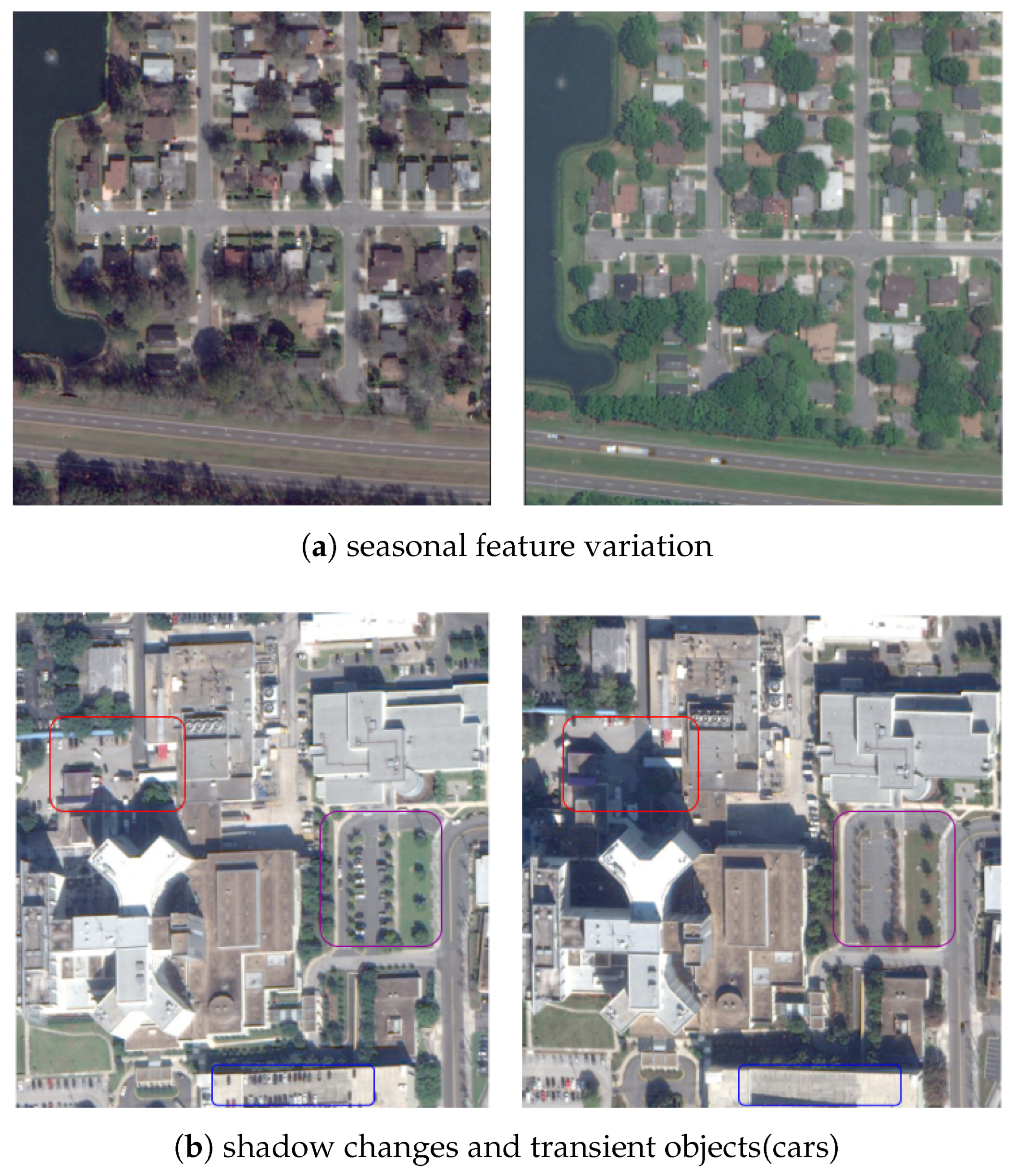
• We propose SatGS, a 3D Gaussian Splatting-based framework with a novel appearance-adaptive adjustment strategy, which facilitates both global and local seasonal variation adjustments, while accurately describing the shape and tone of shadow regions;
• We design a specific uncertainty optimization scheme that enables robust removal of transient objects from a trained scene;
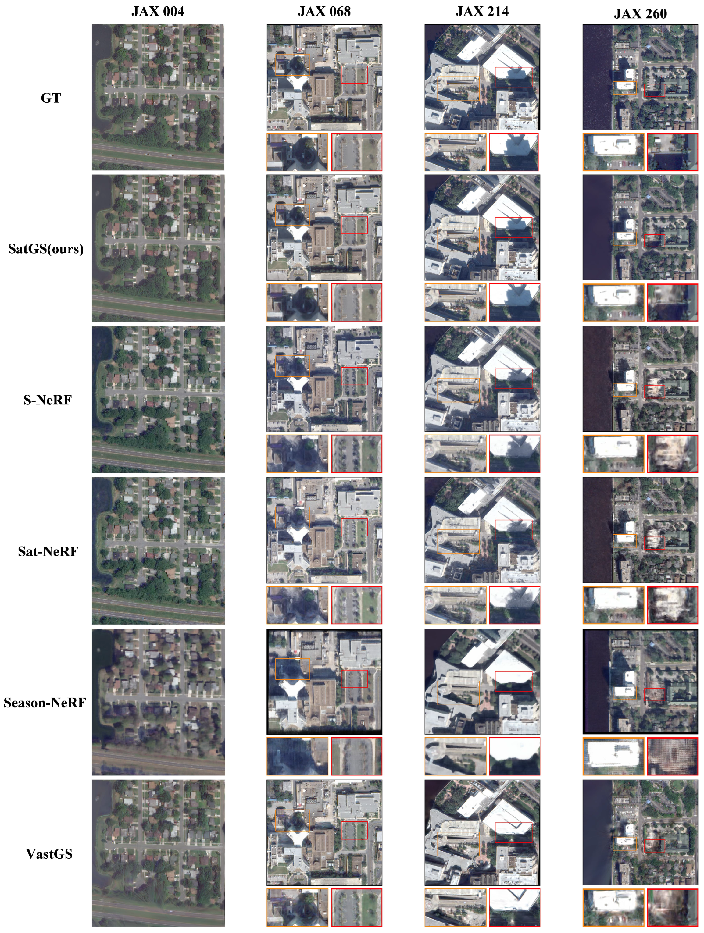
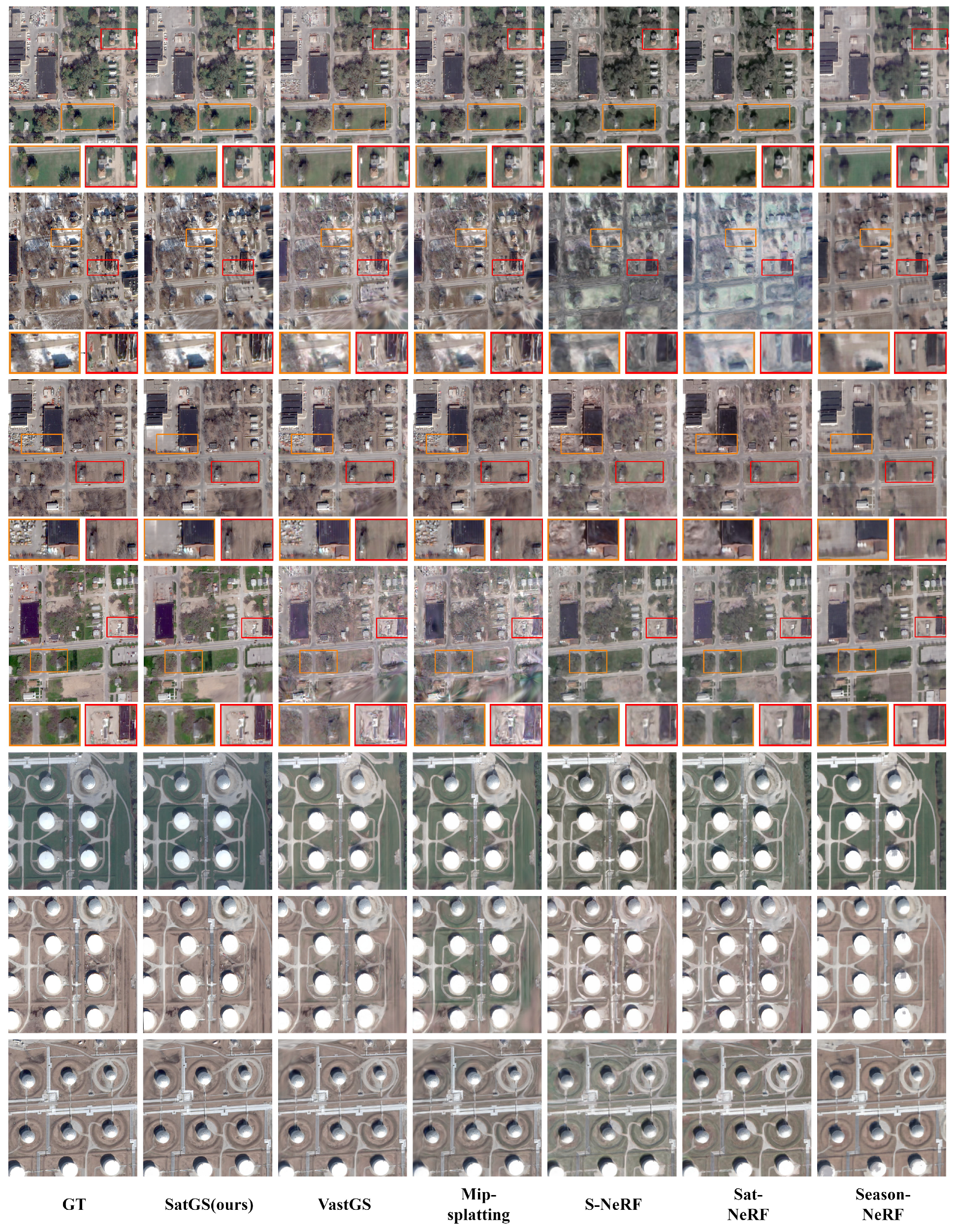
• Experimental results demonstrate that SatGS not only outperforms several State-of-the-Art NeRF-based methods in terms of rendering quality but also surpasses them in rendering speed and training time efficiency.

2. Related Work

2.1. 3D Representation for Novel View Synthesis

Novel view synthesis typically uses rendering techniques to generate new views of a scene, after representing its geometric and appearance information by 3D representations. Implicit and explicit representations are two common methods for scene representation. Implicit representation [1,20,21,22,23,24] often encodes scene information into neural network weights, where 3D coordinates serve as inputs and corresponding 3D geometric details (such as occupancy, signed distance, color, and density) are output. Among these, NeRF [21] is a groundbreaking work that represents complex scenes by learning a radiance field and generates novel, photorealistic views through volume rendering.

In contrast to implicit representation, explicit representation typically describes a 3D scene using a 3D model made up of meshes [25,26,27], point clouds [28,29], or voxels [30]. Recently, 3DGS [9] has rapidly become a hot topic in the field due to its real-time rendering speed while maintaining high-resolution synthesis quality. The newly popularized 3DGS introduces a novel explicit scene representation using 3D Gaussian functions, combining the benefits of neural network-based optimization and explicitly structured data storage. With its efficient tile-based rasterizer, 3DGS accelerates rendering speed significantly compared to previous methods. Building upon 3DGS, Mip-Splatting [31] introduces an innovative filtering framework that integrates both 3D smoothing filters and 2D mip filters. This dual-filter architecture effectively mitigates aliasing artifacts while substantially improving rendering fidelity, a methodological advancement that has subsequently been widely adopted in subsequent research [31,32,33,34,35,36,37].

2.2. Novel View Synthesis for Unstructured Photo Collections

In real-world scenes, a large portion of the multi-view images we can obtain belong to unstructured photo collections, such as multi-date satellite collections [38] or internet photo collections [39]. These images are typically captured with different settings at different times, and are characterized by significant appearance variations (e.g., varying lighting, seasonal changes) as well as the presence of transient objects (e.g., pedestrians and vehicles). When performing novel view synthesis using these unstructured photo collections, challenges arise due to the inherent inconsistencies within the datasets. NeRF in the Wild (NeRFW) [40] pioneered solutions for handling appearance variations by incorporating a learnable appearance embedding within the MLP. Recognizing that not all observed pixel colors are equally reliable due to the presence of transient objects, NeRFW allows for an uncertainty field to be emitted for transient parts. This enables the model to adjust the reconstruction loss accordingly, ignoring unreliable pixels and 3D locations that may contain occlusions. Subsequent works [39,41,42,43] followed NeRFW’s strategy and extended it in various ways.

S-NeRF [4] and its extension, SatNeRF [5], are specifically designed for satellite imagery. Leveraging the solar angle information provided by satellite data, they train a Shadow Neural Radiance Field to predict changes in shadows as the solar angle varies. As S-NeRF and SatNeRF have demonstrated the effectiveness of shadow modeling in improving rendered image quality, we have also incorporated similar shadow modeling to handle varying shadows in our work. SeasonNeRF [8] builds upon S-NeRF and SatNeRF by introducing time as an additional variable, enabling the network to render seasonal features.

Recent concurrent works have begun to explore the replacement of NeRF representations with 3DGS for this task. To improve 3DGS performance in unconstrained setting, GS-W [16] employs a CNN to extract independent appearance features for 3D Gaussian points, ensuring that the appearance of each point is conditioned on a reference image. VastGaussian [10] embeds a learnable embedding into each downsampled pixel of the rendered image, feeding it into a CNN to generate a transformation map for appearance adjustment. SWAG [44] utilizes a hash grid to encode the center of each Gaussian, inputting this position encoding along with each image’s embedding into an MLP to generate image-conditioned colors for the 3D Gaussian points. WildGaussians [15] embeds a trainable embedding vector for each 3D Gaussian point and employs a tone-mapping MLP, enabling the rendered image to be conditioned on a specific input image’s embedding. VastGS [10] propose a spatial partitioning strategy for large-scale drone dataenabling parallel scene training and a decoupled appearance modeling approach specifically designed to address illumination variations characteristic of aerial scene. This strategy maintains real-time rendering performance while effectively handling the challenging uneven illumination conditions prevalent in drone-captured environments. Existing 3DGS-based methods designed for unstructured collections adjust the appearance of rendered images by incorporating appearance features based on reference images. This technique effectively handles global appearance changes, yet it struggles to manage the varying shadow regions in satellite images. This is likely because these appearance features fail to accurately capture the detailed information of the shadows.

3. Method

We propose SatGS in this paper, a 3DGS variant aiming to extend 3DGS to satellite content for high-quality, new view reconstruction and real-time rendering. As illustrated in Figure 2, SatGS begins with multi-view and multi-date satellite images and their corresponding initial RPC camera models, followed by an initialization process to obtain approximate pinhole cameras of the RPC cameras, initial point clouds and per-image embedding. Subsequently, we obtain a 3DGS representation capable of simultaneously adapting to seasonal variations and shadow changes through appearance adaptive adjustment. To mitigate the impact of transient objects on reconstruction quality, uncertainty modeling generates and refines a visibility map to mask these object pixels. Regions with lower visibility will be disregarded to avoid larger losses.

In Section 3.2, we show how to initialize SatGS. In Section 3.3, we will introduce how to achieve appearance adaptive adjustment through shadow modeling and appearance modeling. We also show in Section 3.3 how we can make shadow modeling work better and avoid interference between appearance modeling and shadow modeling through loss design. In Section 3.4, we elaborate the composition and function of uncertainty modeling. Section 3.5 presents the final loss used for training SatGS.

3.1. Preliminaries

Our method is based on 3D Gaussian splatting(3DGS), where the scene is explicitly represented by a set of 3D Gaussian points $G_i$. $G_i$ is given as:

$$G_i(x-{\mu }_i,\sum )=e^{-{\displaystyle \frac{1}{2}}{(x-{\mu }_i)}^T{\sum }_i^{-1}(x-{\mu }_i)}$$

(1)

where ${\mu }_i$ represents the position of $G_i$, initialized using a point cloud obtained through Structure from Motion(SfM) [45]. ${\sum }_i$ is the 3D covariance matrix, characterizing the configuration of each $G_i$. ${\sum }_i$ is composed of a scaling matrix S and a rotation matrix R:

$${\sum }_i=RS{S}^T{R}^T$$

(2)

The scaling matrix S and rotation matrix R are stored as Gaussian point attributes—scale s and rotation r—using 3D vectors and quaternions, respectively. In addition to s and r, each $G_i$ also has two other attributes: opacity ${\alpha }_i$ and color $c_i$. The color $c_i$ is initialized using the colors from the SfM point cloud and represented using third-order spherical harmonic coefficients. During rendering, the 3D Gaussians are projected onto the 2D image plane within 16 × 16 pixel tiles, forming 2D Gaussians. The expression for 2D Gaussians is similar to that of 3D Gaussians, with their covariance ${\sum }_i^{\prime }$ given as:

$${\sum }_i^{\prime }=\left(\begin{array}{c}JW{\sum }_i{W}^T{J}^T\end{array}\right)$$

(3)

where W is the viewing transformation matrix, which is also used to project the 3D Gaussian positions ${\mu }_i$ onto the 2D plane to obtain the 2D Gaussian positions ${\mu }_i^{\prime }$. J is the Jacobian of an affine approximation of W. After obtaining the 2D Gaussians $G^{2D}$, they are sorted based on the depth of the original 3D Gaussians(distance from the 3D Gaussian position to the image plane). The view-dependent colors $c_i$ of each 2D Gaussian are alpha-blended to obtain the color of each pixel according to the sorting order $1,\dots ,K$:

$$\widehat{C}=\sum _{i=1}^K{c}_i\left(\mathbf{r}\right){\alpha }_i{G}_i^{2D}\left(\mathbf{r}\right)\prod _{j=1}^{i-1}(1-{\alpha }_j{G}_j^{2D}\left(\mathbf{r}\right))$$

(4)

The loss function for 3DGS is a weighted sum of the L1 loss and the DSSIM loss [46], calculated based on the predicted color $\widehat{C}$ and the ground truth color $C_{gt}$ from the training images, using a hyperparameter $\lambda$:

$$\mathcal{L}=(1-\lambda ){\mathcal{L}}_1(\widehat{C},C_{gt})+\lambda {\mathcal{L}}_{\mathrm{D}-\mathrm{SSIM}}(\widehat{C},C_{gt})$$

(5)

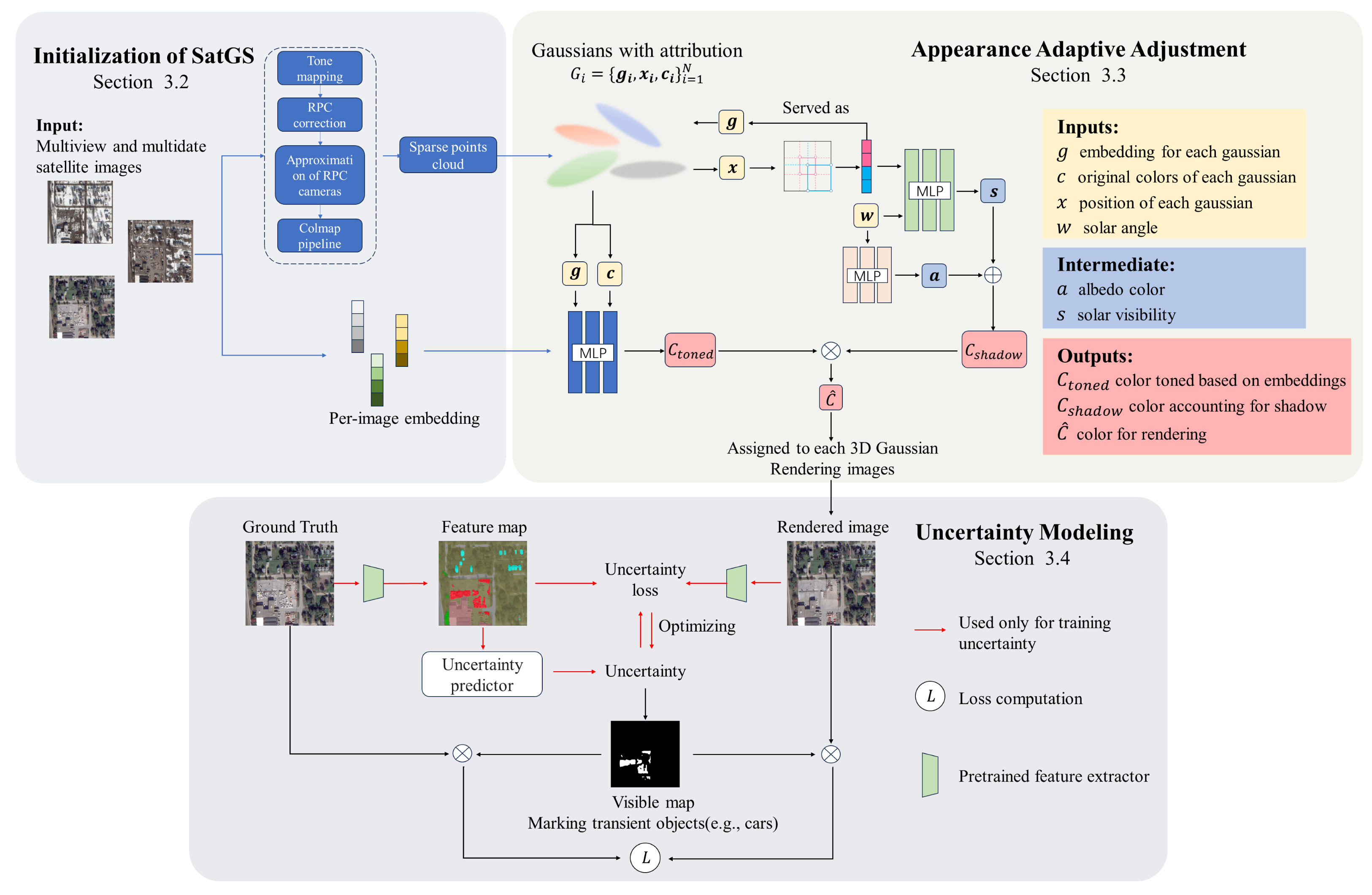
3.2. Initialization of SatGS

To adapt 3DGS to satellite imagery, we first require initial point clouds of the satellite scene and a projection matrix to project the 3D Gaussians onto the 2D image plane. Previous work [9,47] often utilizes Structure-from-Motion(SfM) pipelines like COLMAP [45] to recover accurate camera parameters, generating both the projection matrix and the initial point clouds. However, the discrepancy between camera models (RPC vs.pinhole) prevents direct use of satellite imagery in COLMAP. While reconstructing a sparse point cloud by handling epipolar lines described by the RPC model is possible [48], this approach is computationally complex. Fortunately, ref. [49] mathematically demonstrates the feasibility of locally approximating RPC models with pinhole camera models and provides a numerical method for estimating the necessary camera parameters. With such a perspective projection matrix, standard SfM pipelines can then be employed to obtain the sparse point clouds and a refined projection matrix required for 3DGS.

Our initialization process follows these steps: First, we extract the RPC model parameters from the satellite data and tonemap the high dynamic range(HDR) imagery to LDR by gamma correction to accelerate computations. Next, we utilize the method from [49] to perform a local approximation of the RPC model. To minimize errors introduced by this approximation, we correct the RPC models of all images using the method described in [50] before approximation. We then use the 3D-2D correspondences obtained during this bundle adjustment process to solve for the approximate perspective projection matrix of the RPC model. The corrected perspective projection matrix and the refined 2D feature points are then input into COLMAP to reconstruct sparse point clouds and obtain more accurate projection matrix. We initialize the 3D Gaussian points using these sparse point clouds and assign each Gaussian an additional trainable embedding ${\mathbf{g}}_i$. Each image is also assigned a learnable embedding ${\mathbf{e}}_i$, optimized alongside the ${\mathbf{g}}_i$ during training.

3.3. Appearance Adaptive Adjustment

3.3.1. Appearance Modeling

Seasonal characteristic variations are typically global changes. Therefore, we can capture these seasonal variations by introducing a learnable global feature embedding ${\mathbf{e}}_i$ for each training image. Additionally, we observe that seasonal variations can also exhibit local differences, such as partial snow cover in some areas while other regions remain snow-free. These local variations align with the overall seasonal characteristics but exhibit subtle differences depending on their spatial location. To account for this, we assign each Gaussian point a local embedding ${\mathbf{g}}_i$ based on positional feature information modeled by a multi-resolution hash network, allowing it to fine-tune the global appearance features and activate different colors under different appearances to adapt to local seasonal differences. The ${\mathbf{g}}_i$ and ${\mathbf{e}}_i$, along with the 0th-order spherical harmonic SH features of the Gaussian point, are fed into an MLP with two hidden layers to predict an affine color transformation with coefficients $\beta$ and $\gamma$. By applying this affine transformation to the view-dependent color $c_i\left(\mathbf{r}\right)$ of each Gaussian, we obtain the toned color ${\mathbf{c}}_{\mathbf{toned}}$, which models appearance variations:

$${\mathbf{c}}_{\mathbf{toned}}=\gamma ·c_i\left(\mathbf{r}\right)+\beta$$

(6)

Such an appearance modeling approach effectively captures seasonal features that exhibit global variations across training images, while allowing each Gaussian to fine-tune for local appearance changes.

3.3.2. Shadow Modeling

Appearance modeling does not always successfully account for the movement of shadows and variations in lighting, as these pattern changes are primarily caused by shifts in the light source, specifically the movement of the sun, which alters both the direct light source (the sun) and the indirect light source (reflected light from the sky). S-NeRF [4] demonstrates how to model these two light sources by leveraging local positional information of the scene and solar angle information, thereby successfully avoiding color and structural errors in shadowed regions. We modified this shadow radiance field to make it compatible with 3DGS and incorporate it into our appearance-adaptive adjustment strategy. Specifically, our shadow modeling employs an MLP that takes the hash-encoded positions x of the 3D Gaussian points and the solar angle $\omega$ as input to predict a solar visibility value $s(x,\omega )$ for each Gaussian point. The hash encoding method is adopted from Instant-NGP [51]. We use another MLP to predict the ambient light value $\mathbf{a}\left(\omega \right)$, based on the solar angle $\omega$. We then compute the shadow color for each Gaussian by a weighted sum of a white light source ${\mathbb{I}}_3$ and predicted the ambient light value by Equation (7). The term ${\mathbb{I}}_3$ represents a unit vector characterizing the Sun emits white light in the visible bands.

$${\mathbf{c}}_{\mathbf{shadow}}=s{\mathbb{I}}_3+(1-s)·\mathbf{a}$$

(7)

Finally, we obtain the final color used for rendering by the point-wise product of the toned color and the shadow color:

$$\widehat{\mathbf{c}}={\mathbf{c}}_{\mathbf{shadow}}·{\mathbf{c}}_{\mathbf{toned}}$$

(8)

We now explain how Equations (7) and (8) to simultaneously achieve seasonal and shadow adjustments. In Equation (7), $\mathbf{a}$ represents the bluish hues for shadows predicted based on the solar angle. The variation in shadow hues arises from changes in the sky’s reflection of sunlight, which depends solely on the solar angle. Meanwhile, s evaluates the degree to which each Gaussian point is illuminated by the sun, influenced by the Gaussian point’s position, opacity, and the current solar angle. The value of s ranges from 0 to 1, with higher values indicating greater visibility to the sun and thus a lesser contribution to shadow formation. In Equation (8), ${\mathbf{c}}_{\mathbf{shadow}}$ adjusts ${\mathbf{c}}_{\mathbf{toned}}$ by darkening it according to the current shadow hue, thereby achieving shadow adjustment on top of seasonal adjustment. This approach is based on the observation that while the formation of shadows is not strongly correlated with seasonal changes, the tone of shadow regions is influenced not only by $\mathbf{a}$ but also by seasonal characteristics. Ideally, when $s\approx 1$, ${\mathbf{c}}_{\mathbf{shadow}}\approx 1$, indicating that the Gaussian point is fully illuminated by the sun and casts no shadow. Consequently, the color of this Gaussian point should be entirely determined by the seasonally adjusted color ${\mathbf{c}}_{\mathbf{toned}}$. Conversely, when $s\approx 0$, the Gaussian point lies entirely within the shadowed region, and its color should be solely determined by the predicted shadow hue.

It is also noteworthy that we employ the feature information output by the multi-resolution hash encoding network as the shared input for both appearance modeling and shadow modeling. These positional feature information provide a locality prior for appearance modeling, thereby enhancing generalization capability and accelerating convergence speed, while also avoiding the use of excessively deep MLPs in shadow modeling to extract positional features thus improve training efficiency. In addtion to that, by sharing feature representations, the learning processes of the two modules are coordinated, and gradients from the loss function can be effectively propagated to both modules, thereby promoting their joint optimization.

3.3.3. Additional Loss Terms

To make shadow modeling work better and prevent the toned color from overriding the shadow color, we introduce three additional loss terms:

$${\mathcal{L}}_{sc}={\displaystyle \frac{1}{N}}\sum _{i=1}^N{(s_i-T_i)}^2$$

(9)

$$T_i=\prod _{j=1}^{i-1}(1-{\alpha }_j{G}_j^{2D}\left(\mathbf{r}\right))$$

(10)

$${\mathcal{L}}_{toned}={\displaystyle \frac{1}{N}}\sum _{i=1}^N{\left(1-{\displaystyle \frac{min\left({\mathbf{c}}_{\mathbf{toned}},\mathbb{T}\right)}{\mathbb{T}}}\right)}^2$$

(11)

$${\mathcal{L}}_s=\sum _{i=1}^3\left\{\begin{array}{cc}0\hfill & a_i\le \eta \hfill \\ {\left({\displaystyle \frac{1}{\eta }}\ast a_i-1\right)}^2\hfill & a_i>\eta \hfill \end{array}\right.$$

(12)

where N denotes the total number of Gaussian points, $s_i$ denotes the predicted solar visibility for the i-th Gaussian point, ${\alpha }_j$ and $G_j^{2D}$ represent the opacity and corresponding 2D Gaussian distribution of the j-th Gaussian point, respectively, and $T_i$ indicates the transparency for the i-th Gaussian point, computed via Equation (10). In Equation (12), the subscript i denotes the index of the color channel, while $a_i$ represents the predicted ambient light value for the i-th color channel. The first term is introduced to ensure the solar visibility $s_i$ of each Gaussian point proportional to its transparency $T_i$. The idea behind ${\mathcal{L}}_{toned}$ is to encourage toned color to have higher values than the shadow color, thus preventing the model from relying solely on the toned color to represent shadowed regions. We observed that shadows are typically learned as tones with values often below 0.23 across all channels. Therefore, we set the hyperparameter $\mathbb{T}$ to 0.23. We use ${\mathcal{L}}_s$ to prevent the model from trivially minimizing the loss by setting $a_i$ to 1. We deliberately avoided employing the L2-norm of the ambient light value $a_i$ as the loss function, as this formulation would drive $a_i$ towards zero, which in turn would result in excessively dark shadow regions that completely exclude seasonally adjusted colors. In reality, we have observed that seasonally toned color can partially capture the feature representations of shadow regions (for example, the shadow tone in a snowy area should be consistent with that area to a certain extent). Therefore, we use the hyperparameter $\eta$ to control the extent to which the model suppresses the contribution of toned color in explaining shadow regions. We set eta to 0.5 which ensures that shadowed areas reduce the influence of seasonally adjusted colors by at least 50%, while still allowing some indirect light to illuminate the region. By using ${\mathcal{L}}_{toned}$ and ${\mathcal{L}}_s$ it helps ensure that shadow regions are predominantly explained by shadow-specific features, while still allowing toned color to contribute to a limited extent, thus maintain the relative strength of the shadows and toned colors.

The complete loss function ${\mathcal{L}}_{AS}$ for appearance and shadow modeling is:

$${\mathcal{L}}_{AS}={\mathcal{L}}_{sc}+{\mathcal{L}}_{toned}+{\mathcal{L}}_s$$

(13)

3.4. Uncertainty Modeling

While our appearance adaptive adjustment strategy allows for robustness against local variations, artifacts and erroneous geometry can still occur in regions with transient objects (such as moving cars). NeRF-based methods [5,39,40] can mitigate this by incorporating an additional network within their neural radiance field to model uncertainty, effectively discounting losses from challenging pixels. However, this approach is not directly applicable to 3DGS and often requires extensive per-pixel sampling, hindering rendering speed and increasing training costs. To address this, we propose an uncertainty modeling approach tailored for SatGS, decoupled from the 3DGS rendering pipeline and discarded after training to maintain real-time rendering performance. Specifically we first obtain the deep features $F^{\prime }$ of the training image and the deep features F of the rendered image by a pre-trained feature extractor. Then, an uncertainty predictor is employed to take the features $F^{\prime }$ as input to predict uncertainty $\mathit{\sigma }$. We chose Dinov2 [19] from [19,52,53] as our pre-trained feature extractor because it provides more powerful feature extraction capabilities. Given that $F^{\prime }$ already provides semantic information sufficient for segmenting transient and static objects, the predicted uncertainty essentially constitutes an affine transformation of these features. Therefore, we construct a lightweight predictor comprising a 2D convolutional layer with BatchNorm and a softplus activation function. An additional advantage of utilizing Dinov2 features for uncertainty prediction lies in their robustness to appearance variations. This robustness reduces the likelihood of misclassifying regions with illumination changes or seasonal variations as transient object regions, thereby enhancing the reliability of the predicted uncertainties. The idea of leveraging a pre-trained feature extractor for uncertainty modeling is inspired by [16,39]. We then upsample $\mathit{\sigma }$ and use it to create a visibility map:

$$V_m=min({\displaystyle \frac{1}{2{\mathit{\sigma }}^2}},1)$$

(14)

We apply this visible map to Equation (5) to form the loss used to optimize SatGS:

$$\begin{array}{ccc}{\mathcal{L}}_{\mathrm{mask}}\hfill & =\hfill & (1-\lambda ){\mathcal{L}}_1(V_m\odot \widehat{C},V_m\odot C_{gt})\hfill \\ & & +\lambda {\mathcal{L}}_{\mathrm{D}-\mathrm{SSIM}}(V_m\odot \widehat{C},V_m\odot C_{gt})\hfill \end{array}$$

(15)

where ⊙ denotes the element-by-element product. The visibility map $V_m$ is utilized to identify and suppress the visibility of transient object regions. During training, the $L_{\mathrm{mask}}$, weighted by $V_m$, places greater emphasis on regions with high visibility while disregarding those with low visibility, therefore minimizing the influence of transient objects.

We train the visibility map with the following uncertainty loss:

$$\begin{array}{cc}\hfill {\mathcal{L}}_{\mathrm{uncertainty}}=& {\displaystyle \frac{\mathrm{Similarity}(F,F^{\prime })}{2{\mathit{\sigma }}^2}}+{\lambda }_{\mathrm{prior}}log\mathit{\sigma }\hfill \\ \hfill & +\parallel 1-{\displaystyle \frac{1}{2{\mathit{\sigma }}^2}}{\parallel }_2^2\hfill \end{array}$$

(16)

where similarity is calculated as:

$$\mathrm{Similarity}(F,F^{\prime })=min\left(1,{\lambda }_p-{\displaystyle \frac{{\lambda }_{p}F·F^{\prime }}{{\parallel F\parallel }_2{\parallel F^{\prime }\parallel }_2}}\right)$$

(17)

Equation (17) equals zero when the cosine similarity between these two features is 1, and gradually increases as the feature cosine similarity decreases. In practice, when the feature cosine similarity drops below 0.5, it strongly indicates that the corresponding pixels likely belong to transient objects. Therefore, We use the hyperparameter ${\lambda }_p$ to control the proportion of uncertainty regions and speed up convergence. ${\lambda }_p$ is set to 2, which means Equation (17) stops increasing linearly and directly reaches 1 when the cosine similarity falls below 0.5. This parameter configuration amplifies the uncertainty loss for dissimilar samples, thereby improving training efficiency. The second term prevents the uncertainty from collapsing to infinity, while the third term prevents the visibility map from marking all pixels as invisible. This loss is exclusively used to optimize the uncertainty and gradients are not propagated back into the SatGS rendering pipeline.

3.5. Loss Function

We train SatGS using a combination of Equations (13) and (15) as our loss function. In addition to these two terms, we also incorporate the perceptual loss [54], as we found it improves performance without impacting convergence speed. Following the approach in [32,55], we accumulate gradients of the 2D Gaussian positions using the absolute values of the gradients rather than the actual gradient values during backpropagation. The total loss function is formulated as shown below, where $\lambda$ used in ${\mathcal{L}}_{mask}$ is set to 0.2 and ${\lambda }_{LPIPS}$ is set to 0.005. These parameter configurations were adopted following the methodology established in previous studies [9,16].

$${\mathcal{L}}_{total}={\mathcal{L}}_{AS}+{\mathcal{L}}_{mask}+{\lambda }_{LPIPS}{\mathcal{L}}_{LPIPS}$$

(18)

4. Experiments

4.1. Experimental Setup

4.1.1. Dataset

We evaluated the performance of SatGS on eight areas of interst(AOIs) of the 2019 IEEE GRSS Data Fusion Contest [38]. This dataset provides high-resolution multi-view satellite imagery of the city of Jacksonville and Omaha. The images are RGB images, 2048 by 2048 pixels in size, covering an area of 580 by 580 m, and include associated RPC information and ground truth lidar-derived digital surface models (DSMs). Following [5], each scene was divided into different AOIs. Each AOI was cropped from the original RGB images to a resolution of approximately 800 by 800 pixels, covering a 256 by 256 m area. The index of each region and the training/test set splits are detailed in

Table 1. Number of input images used for Jacksonville area.

Area Index	JAX 004	JAX 068	JAX 214	JAX 260
training/test	9/2	17/2	21/3	15/2

and 

Table 2. Number of input images used for Omaha area.

Area Index	OMA 163	OMA 203	OMA 212	OMA 281
training/test	40/5	43/6	38/6	41/6

. These scenes encompass complex textured regions such as vegetation, urban buildings, and water bodies. The corresponding image collections exhibit appearance inconsistencies, including seasonal variations, shadow shifts, and transient objects. Notably, the four scenes from Omaha demonstrate more pronounced seasonal variations due to a longer time span of image acquisition, while the Jacksonville scenes exhibit significant shadow displacement. We also provide reconstruction results for the undivided regions with original high resolution(2048 by 2048 pixels). We use bundle-adjusted RPCs of all images acquired by the method described in [50].

4.1.2. Implementation Details

Our model is implemented using the Mip-Splatting renderer (GitHub repository: https://github.com/autonomousvision/mip-splatting) [31] and trained on a single Nvidia RTX 4090 GPU. Most of SatGS’s learning rate settings follow those of Mip-Splatting. We use the Adam optimizer [56], with the following differences in learning rates: the learning rates for the MLPs used in appearance and shadow modeling are set to 0.0005, the image appearance embedding learning rate is set to 0.001, and the uncertainty learning rate is also set to 0.001. The optimization scheme for hash encoding follows Instant-NGP [48,51]. Uncertainty modeling is not applied until after 35,000 steps, with an additional 5000-step warm-up training.

4.1.3. Evaluation Metrics

To assess the quality of novel view synthesis, we used peak signal-to-noise ratio (PSNR), structural similarity index (SSIM) [46], and learned perceptual image patch similarity (LPIPS) [54] as evaluation metrics, following common practice. We compared the training times of the different models in GPU hours, as well as rendering times, in frames per second (FPS), to evaluate their efficiency.

4.2. Evaluation Scheme

In the proposed method, we optimize the appearance embeddings only for images in the training set. To evaluate images in the test set, the corresponding embedding must be identified to achieve accurate appearance adjustment. To address this issue, we use a test-time optimization method similar to [57], where an embedding is assigned to each test image, and an additional training process is introduced in test time. During this process, the other parts of the model remain fixed, and we employ the Adam optimizer [56] with Equation (5) as the loss function to optimize only the embedding for the test image. The test-time optimization are summarized in Algorithm 1. $N_{\mathrm{epochs}}$ is set to 5000. It is noteworthy that the uncertainty modeling module is discarded after the training phase and does not participate in the evaluation process.

Algorithm 1 Test-time Optimization
I: Set of test images
$\mathcal{M}$: Pretrained SatGS model (parameters fixed)
$\mathbf{E}=\left\{{\mathbf{e}}_i\right\}$: Learnable image embeddings
$\mathbf{W}=\left\{{\omega }_i\right\}$: Solar angles
Initialize $\mathbf{E}$	▹ Random initialization
for epoch $=1$ to $N_{\mathrm{epochs}}$ do
for image $I_i\in I$ do
${\mathbf{e}}_i\leftarrow \mathbf{E}\left[i\right]$
${\omega }_i\leftarrow \mathbf{W}\left[i\right]$
${\widehat{I}}_i\leftarrow \mathrm{Render}(\mathcal{M},{\mathbf{e}}_i,{\omega }_i)$	▹ Only ${\mathbf{e}}_i$ and ${\omega }_i$ affect output
$\mathcal{L}\leftarrow Loss({\widehat{I}}_i-I_i)$	▹ Equation (5)
${\mathbf{e}}_i\leftarrow \mathrm{Adam}\left({\nabla }_{\mathcal{L}}\right)$	▹ Only update current embedding
end for
end for
return ${\mathbf{E}}^{*}\leftarrow \mathbf{E}$

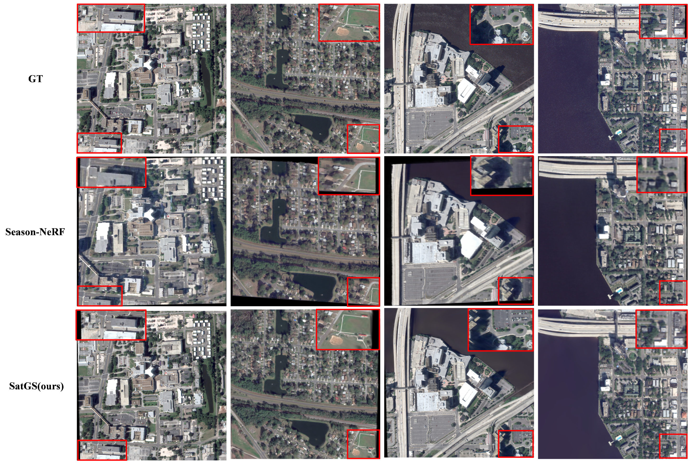
4.3. Comparison to State-of-the-Art Methods

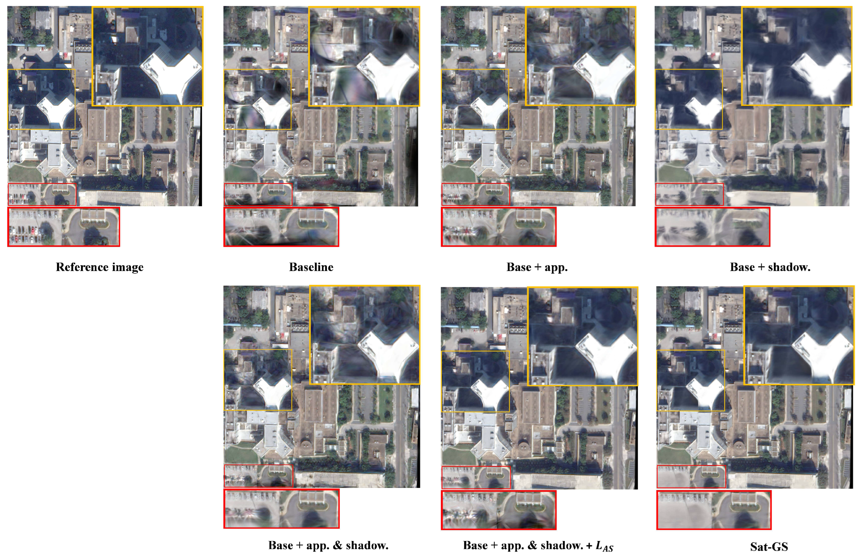
We compare our method with three State-of-the-Art(SOTA) novel view synthesis methods designed for satellite remote sensing scene: S-NeRF [4], Sat-NeRF [5], Season-NeRF [8]. We also incorporate three 3DGS-base methods into our comparison, which includes the original 3DGS [9], Mip-Splatting [31] and VastGaussian(VastGS) [10]. S-NeRF is the first try to extend the original NeRF to multi-date satellite collections by incoporating the solar information into the network to learn the directional illumination from the sun and indirect illumination from a diffuse light source. Sat-NeRF further improved S-NeRF’s performance by using uncertainty modeling and introducing a RPC-based sample stragety. Season-NeRF build upon S-NeRF and Sat-NeRF, specifying seasonal features by introducing time variable. Three-dimensional Gaussian Splatting introduces 3D Gaussians as a novel and flexible scene representation and designs a fast differentiable rendering approach, enabling real-time rendering while maintaining high-fidelity view synthesis. Building upon the framework of 3DGS, Mip-Splatting incorporates 3D smoothing filters and 2D mip filters, effectively reducing aliasing artifacts and significantly enhancing rendering quality. However, both 3DGS and Mip-Splatting assume scenes under controlled settings without appearance variations. This assumption limits their applicability to satellite scenes. To address the appearance variations in drone-captured remote sensing scenarios, VastGS introduces decoupled appearance modeling into the optimization process to reduce appearance variations in rendered images. However, we will show that the appearance modeling approach of VastGS is insufficient to handle the more pronounced seasonal appearance variations present in satellite remote sensing scenarios.

Figure 3 show the qualitative comparison between SatGS and other SOTA methods in Jacksonville area. Image collections for this area shows complex appearance variations, simultaneously including global tone variations due to seasonal changes, shadow changes caused by the movement of the sun and other local appearance variations. We can observe that the images rendered by SatGS exhibit greater clarity in the edges and textures of objects and are closer to the ground truth. The comparative results on AOI 168, 214, and 260 demonstrate that SatGS is capable of rendering higher-quality shadows while exhibiting stronger robustness against variations in vegetation and buildings within the scene. The comparison on AOI 004 shows that the overall tone of the images rendered by SatGS is more consistent with the ground truth.

Figure 4 presents a qualitative comparison between SatGS and other SOTA methods in the Omaha area. The image collections for this area span a longer time period, resulting in more pronounced seasonal variations. We can observe that in complex regions with shadow and seasonal variations, Mip-Splatting exhibits noticeable blurring and severe artifacts. Even in relatively simpler regions, Mip-Splatting shows significant errors in the texture and color of vegetation. VastGS-style appearance modeling proves inadequate for handling scenes in the Omaha region, which renders vegetation with incorrect colors and introduces noticeable artifacts in certain complex areas. Both S-NeRF and SatNeRF also fail to adapt to seasonal variations, with only SeasonNeRF and our method successfully adjusting the appearance according to seasonal changes. However, SeasonNeRF’s appearance adjustment comes at the cost of reduced rendering quality, resulting in blurred edges and loss of detail in the rendered images. In contrast, SatGS achieves accurate adaptive appearance adjustment while preserving precise texture details.

Quantitative evaluations of different methods are given in

Table 3. Numerical results for Jacksonville area using the test images (unseen in training). Bold values indicate the best results.

	PSNR↑				SSIM↑				LPIPS↓				GPU hrs./
	004	068	214	260	004	068	214	260	004	068	214	260	FPS (Mean)
S-NeRF (2021)	25.87	24.2	24.51	21.52	0.864	0.901	0.939	0.829	0.262	0.130	0.251	0.326	6.2/0.11
Sat-NeRF (2022)	26.15	25.27	25.51	21.90	0.877	0.913	0.951	0.840	0.270	0.141	0.260	0.342	8.0/0.13
Season-NeRF (2024)	24.06	22.63	23.69	21.48	0.659	0.710	0.785	0.612	0.328	0.349	0.331	0.336	3.5/0.002
3DGS (2023)	17.41	16.48	16.31	16.00	0.420	0.565	0.645	0.442	0.494	0.334	0.349	0.501	1.2/113
Mip-Splatting (2024)	20.16	17.20	18.87	18.51	0.570	0.588	0.645	0.542	0.398	0.318	0.414	0.486	1.8/108
VastGaussian (2024)	22.08	21.41	22.74	20.18	0.672	0.747	0.735	0.651	0.316	0.223	0.256	0.364	2.8/56
Sat-GS (Ours)	30.57	26.41	26.43	25.82	0.880	0.928	0.925	0.864	0.193	0.129	0.142	0.218	2.5/81

and

Table 4. Numerical results for Omaha area using the test images (unseen in training). Bold values indicate the best results.

	PSNR↑				SSIM↑				LPIPS↓				GPU hrs./
	163	203	212	281	163	203	212	281	163	203	212	281	FPS (Mean)
S-NeRF (2021)	19.23	20.00	20.35	18.50	0.539	0.629	0.672	0.551	0.514	0.452	0.379	0.594	6.5/0.11
Sat-NeRF (2022)	19.26	20.49	19.71	19.02	0.566	0.658	0.679	0.582	0.512	0.434	0.359	0.565	7.2/0.118
Season-NeRF (2024)	19.82	21.44	20.26	20.99	0.591	0.660	0.640	0.642	0.457	0.372	0.328	0.331	4.8/0.03
3DGS (2023)	13.47	14.21	12.60	13.95	0.495	0.559	0.536	0.443	0.575	0.432	0.487	0.696	1.5/86
Mip-Splatting (2024)	15.51	16.84	14.20	16.21	0.460	0.570	0.510	0.477	0.451	0.416	0.536	0.301	2.2/71
VastGaussian (2024)	15.76	17.60	13.71	16.17	0.480	0.603	0.510	0.504	0.460	0.404	0.549	0.298	2.1/63
Sat-GS (Ours)	22.09	23.10	22.62	21.39	0.730	0.779	0.753	0.664	0.291	0.299	0.306	0.290	2.5/77

. In most regions, SatGS is able to produce higher quantitative accuracy compared to other methods in terms of PSNR, SSIM, and LPIPS. The higher LPIPS score of SatGS indicates its superior capability in accurately recovering complex textures, resulting in reconstructions that are closer to the ground truth. Particularly in the Omaha region, which is characterized by intricate textures, significant appearance variations, and numerous transient objects, the higher LPIPS value of SatGS demonstrates its robustness against these challenging factors, effectively minimizing distortions in textures and local details. The higher PSNR of SatGS reflects its greater accuracy in pixel-level reconstruction, with reduced noise and minimal information loss. This is especially evident in Region 004, which contains extensive vegetation. Due to temporal differences in image acquisition, the vegetation exhibits drastic appearance variations across the dataset. The higher PSNR of SatGS in this region highlights the effectiveness of its appearance-adaptive strategy, which mitigates the impact of vegetation appearance differences and avoids the introduction of noise. In terms of SSIM, SatGS achieves lower scores only in the 214 region but outperforms other methods in all other regions. This underscores its advantage in precisely restoring structural information of the scene. Among NeRF-based methods, SeasonNeRF demonstrates better performance in the Omaha region, where seasonal appearance variations are more pronounced, highlighting its superior capability in approximating seasonal changes. However, it still falls short of SatGS across all evaluation metrics. While VastGS-style appearance modeling performs well in the Jacksonville area, showing improvements over the original 3DGS and Mip-Splatting in various metrics, it fails to achieve similar results in the Omaha region.

In terms of efficiency in optimization and rendering, methods based on 3DGS significantly outperform those based on NeRF. It is evident that SeasonNeRF exhibits significantly slower rendering speeds compared to other methods. This is primarily due to its reliance on an additional deep network to predict seasonal colors based on temporal variables, which further exacerbates the already slow rendering speed inherent to the NeRF framework. In contrast, while SatGS also incorporates additional networks, the use of multi-resolution hash encoding and a pre-trained feature extractor ensures that these additions do not substantially hinder its training and rendering speeds. In the Omaha region, SatGS achieves faster rendering speeds than other 3DGS-based methods. This improvement can be attributed to SatGS’s appearance-adaptive capability and transient object removal mechanism, which eliminate the need for additional 3D Gaussian ellipsoids to model appearance variations and transient object regions, thereby enhancing its rendering efficiency.

4.4. Ablation Study

To demonstrate the effectiveness of each component of our method, we conducted an ablation study. We use Mip-Splatting as our baseline and progressively add different modules from our method. The quantity results are presented in

Table 5. Ablation study of each component of SatGS. Bold values indicate the best results.

	PSNR↑				SSIM↑				LPIPS↓
	004	068	214	260	004	068	214	260	004	068	214	260
baseline	20.16	17.20	18.87	18.51	0.570	0.588	0.645	0.542	0.398	0.318	0.414	0.486
+ shadow.	26.03	23.63	22.63	23.85	0.801	0.844	0.809	0.751	0.252	0.156	0.210	0.326
+ app.	26.40	23.51	21.12	22.20	0.833	0.844	0.775	0.733	0.213	0.167	0.225	0.334
+ shadow. & app.	17.66	21.87	23.05	16.80	0.424	0.815	0.830	0.455	0.471	0.187	0.174	0.479
+ ${\mathcal{L}}_{AS}$.	30.37	26.01	26.18	25.17	0.838	0.902	0.901	0.840	0.202	0.158	0.140	0.245
+ uncert. (Sat-GS)	30.57	26.41	26.43	25.82	0.880	0.928	0.925	0.864	0.193	0.129	0.142	0.218

, and the qualitative comparisons of novel view synthesis results are shown in Figure 5 and Figure 6. As shown in Table 5, Mip-Splatting alone proves insufficient to handle the significant appearance variations inherent in satellite imagery, leading to a poor performance in terms of PSNR, SSIM, and LPIPS. While both appearance and shadow modeling individually address some aspects of these variations, neither module alone can fully resolve the complexities of these changes. Furthermore, simply combining appearance and shadow modeling without further refinement is ineffective, resulting in unstable performance. While this naive combination shows improvement over individual modules in Area 214, it performs poorly in other areas. This instability arises from interference between the two modules, hindering their individual contributions. By introducing an additional loss term, ${\mathcal{L}}_{AS}$, we enable the shadow modeling component to function more effectively while encouraging a balance between the two modules, mitigating their interference and resulting in a substantial performance boost.

The rendering results in Figure 5 and Figure 6 corroborate these findings above and further illustrate the roles of each component within SatGS. The rendering results of Mip-Splatting exhibit noticeable errors, such as artifacts, glare, and bright blobs, due to the strong illumination changes and shadow shifts present in the dataset. Both appearance and shadow modeling alleviate these artifacts. However, while appearance modeling alone handles most appearance variations and produces sharp images, it struggles to reconstruct changing shadows, leading to poor quality or even erroneous shadow rendering. Shadow modeling fundamentally involves the reconstruction of solar light sources, addressing issues of inconsistent lighting and generating precise and smooth shadows. However, as illustrated in Figure 5 and Figure 6, relying solely on shadow modeling to interpret changes in appearance results in the smoothing out of numerous texture details, leading to phenomena such as blurred building edges. Furthermore, the outcomes of combining appearance modeling with shadow modeling without the application of ${\mathcal{L}}_{AS}$ closely resemble those achieved through appearance modeling alone. This suggests that, in the absence of ${\mathcal{L}}_{AS}$ for balancing, appearance modeling overrides shadow modeling, thereby preventing shadow modeling from delivering its intended effects. By incorporating ${\mathcal{L}}_{AS}$, both appearance and shadow modeling effectively contribute to high-quality novel view synthesis. The uncertainty modeling forces the network to discard unreliable pixels, effectively removing these error-inducing elements. Although this removal might not significantly improve quantitative metrics (as seen in Table 5), it noticeably enhances the visual quality of the rendered images (as shown in the red boxes of Figure 5 and Figure 6).

4.5. High Resolution Results

We evaluated SatGS’s ability to reconstruct full-scale satellite scenes, comparing its performance against SeasonNeRF [8]. We chose SeasonNeRF as our comparison model because, unlike other baselines, it is specifically adjusted to high-resolution imagery. We trained and tested both models using the original resolution RGB satellite images (2048 × 2048 pixels), covering an area of 580 by 580 m. During training, we adjusted the hyperparameters within ${\mathcal{L}}_{AS}$ to accommodate the large-scale scenes, setting $\mathbb{T}$ to 0.15 and $\eta$ to 0.7, while keeping all other hyperparameters consistent. The quantitative results are presented in

Table 6. Numerical Results of full-scale satellite scenes. Bold values indicate the best results.

	PSNR↑				SSIM↑				LPIPS↓				GPU hrs./
	004	068	214	260	004	068	214	260	004	068	214	260	FPS (Mean)
Season-NeRF (2024)	24.02	22.14	20.67	21.73	0.725	0.740	0.675	0.705	0.712	0.587	0.553	0.454	4.5/0.004
3DGS (2023)	18.96	17.31	17.67	16.21	0.525	0.506	0.635	0.505	0.412	0.369	0.469	0.548	1.6/11.6
Sat-GS (Ours)	26.78	25.07	23.97	24.20	0.789	0.793	0.810	0.720	0.308	0.259	0.304	0.407	3.2/5.6

, and the rendered high-resolution images are shown in Figure 7.

Figure 7 demonstrates that SatGS generates sharper novel views compared to SeasonNeRF. The images rendered by SeasonNeRF appear blurry, particularly at building edges and in textured vegetation areas. Furthermore, SeasonNeRF exhibits missing information in certain viewpoints, especially near the edges of the scene. As Table 6 confirms, SatGS outperforms SeasonNeRF across all evaluation metrics. The missing scene content in SeasonNeRF’s reconstructions contributes to its poor LPIPS score. Notably, when rendering high-resolution images at 2048 × 2048 pixels, SeasonNeRF requires an average of four minutes per view, whereas SatGS needs only 0.17 s. This highlights the significant advantage of SatGS in rendering speed, particularly for high-resolution imagery, compared to NeRF-based methods.

5. Discussion

SatGS introduces appearance-adaptive adjustments and uncertainty modeling, enabling it to adapt to varying appearances in training images while effectively mitigating the interference of transient objects in the reconstruction process. This capability allows SatGS to achieve State-of-the-Art (SOTA) results in the task of novel view synthesis for satellite images. Additionally, SatGS significantly outperforms NeRF-based methods in rendering speed and reconstruction quality, demonstrating the promise of 3D Gaussian Splatting (3DGS) for satellite image reconstruction tasks.

In addition to adaptively adjusting the appearance based on the reference image’s appearance features, SatGS can also simulate the seasonal characteristics of a region over time by interpolating time-ordered appearance embeddings and solar angles, similar to the seasonal specificity capability achieved by SeasonNeRF [8]. As shown in Figure 8, SatGS renders images with the expected seasonal features and correct seasonal properties. From spring to summer, the vegetation becomes greener, while in autumn and winter, it turns yellow and brown. Snow begins to appear in winter. This confirms that SatGS can accurately specify the season based on the seasonal features present in the data.

However, SatGS also has limitations. Its uncertainty modeling relies on the accuracy of a pre-trained feature extractor, specifically DinoV2, which does not always provide precise semantic feature information for all transient objects in the scene. As a result, SatGS cannot achieve as thorough removal of transient objects as Season-NeRF. To address this limitation, we plan to explore the use of satellite image fine-tuned pre-trained feature extractors in future work.

6. Conclusions

We introduced SatGS, a 3DGS variant adapted for multi-date collections of multi-view satellite images. SatGS attempts to account for the significant appearance variations in satellite images from two perspectives: Firstly, SatGS captures the appearance features in multi-temporal datasets by utilizing global image encoding and position-based local encoding, and then applies corresponding transformations to the color of each Gaussian point based on these appearance features. Secondly, SatGS incorporates insights from NeRF-related research by re-modeling the solar light source to achieve accurate descriptions of shadowed areas. The combination of these two aspects enables SatGS to achieve precise appearance adaptive adjustment. Additionally, the proposed uncertainty modeling method allows SatGS to ignore pixels in regions with transient objects, thereby reducing their impact on reconstruction. Thanks to the use of these strategies, SatGS achieves State-of-the-Art results in remote sensing novel view synthesis task from satellite imagery. Beyond novel view synthesis, multi-view satellite photogrammetry is another significant task aimed at accurately estimating 3D shapes, such as generating digital surface models (DSMs). Theoretically, SatGS could render depth maps as a byproduct during novel view synthesis according to the method described in 2DGS [47]. These depth maps could then be utilized to form DSMs. However, this study primarily focuses on the novel view synthesis task, and we leave the exploration of SatGS’s potential applications in satellite photogrammetry as future work.

References

1. Wu, Y.; Zou, Z.; Shi, Z. Remote sensing novel view synthesis with implicit multiplane representations. IEEE Trans. Geosci. Remote Sens. 2022, 60, 5627613. [Google Scholar] [CrossRef]
2. Li, Z.; Li, Z.; Cui, Z.; Qin, R.; Pollefeys, M.; Oswald, M.R. Sat2vid: Street-view panoramic video synthesis from a single satellite image. In Proceedings of the IEEE/CVF International Conference on Computer Vision, Montreal, BC, Canada, 11–17 October 2021; pp. 12436–12445. [Google Scholar]
3. Marí, R.; Facciolo, G.; Ehret, T. Multi-date earth observation NeRF: The detail is in the shadows. In Proceedings of the IEEE/CVF Conference on Computer Vision and Pattern Recognition, Vancouver, BC, Canada, 18–22 June 2023; pp. 2035–2045. [Google Scholar]
4. Derksen, D.; Izzo, D. Shadow neural radiance fields for multi-view satellite photogrammetry. In Proceedings of the IEEE/CVF Conference on Computer Vision and Pattern Recognition, Nashville, TN, USA, 19–25 June 2021; pp. 1152–1161. [Google Scholar]
5. Marí, R.; Facciolo, G.; Ehret, T. Sat-nerf: Learning multi-view satellite photogrammetry with transient objects and shadow modeling using rpc cameras. In Proceedings of the IEEE/CVF Conference on Computer Vision and Pattern Recognition, New Orleans, LA, USA, 18–24 June 2022; pp. 1311–1321. [Google Scholar]
6. Zhang, L.; Rupnik, E. Sparsesat-NeRF: Dense depth supervised neural radiance fields for sparse satellite images. arXiv 2023, arXiv:2309.00277. [Google Scholar] [CrossRef]
7. Zhou, X.; Wang, Y.; Lin, D.; Cao, Z.; Li, B.; Liu, J. SatelliteRF: Accelerating 3D Reconstruction in Multi-View Satellite Images with Efficient Neural Radiance Fields. Appl. Sci. 2024, 14, 2729. [Google Scholar] [CrossRef]
8. Gableman, M.; Kak, A. Incorporating season and solar specificity into renderings made by a NeRF architecture using satellite images. IEEE Trans. Pattern Anal. Mach. Intell. 2024, 46, 4348–4365. [Google Scholar] [CrossRef]
9. Kerbl, B.; Kopanas, G.; Leimkühler, T.; Drettakis, G. 3D Gaussian Splatting for Real-Time Radiance Field Rendering. ACM Trans. Graph. 2023, 42, 139. [Google Scholar] [CrossRef]
10. Lin, J.; Li, Z.; Tang, X.; Liu, J.; Liu, S.; Liu, J.; Lu, Y.; Wu, X.; Xu, S.; Yan, Y.; et al. Vastgaussian: Vast 3d gaussians for large scene reconstruction. In Proceedings of the IEEE/CVF Conference on Computer Vision and Pattern Recognition, Seattle, WA, USA, 16–22 June 2024; pp. 5166–5175. [Google Scholar]
11. Liu, Y.; Luo, C.; Fan, L.; Wang, N.; Peng, J.; Zhang, Z. Citygaussian: Real-time high-quality large-scale scene rendering with gaussians. In Proceedings of the European Conference on Computer Vision, Milan, Italy, 29 September–4 October 2024; Springer: Berlin/Heidelberg, Germany, 2024; pp. 265–282. [Google Scholar]
12. Liu, Y.; Luo, C.; Mao, Z.; Peng, J.; Zhang, Z. CityGaussianV2: Efficient and Geometrically Accurate Reconstruction for Large-Scale Scenes. arXiv 2024, arXiv:2411.00771. [Google Scholar]
13. Wang, Y.; Tang, X.; Ma, J.; Zhang, X.; Zhu, C.; Liu, F.; Jiao, L. Pseudo-Viewpoint Regularized 3D Gaussian Splatting For Remote Sensing Few-Shot Novel View Synthesis. In Proceedings of the IGARSS 2024-2024 IEEE International Geoscience and Remote Sensing Symposium, Athens, Greece, 7–12 July 2024; pp. 8660–8663. [Google Scholar]
14. Lian, H.; Liu, K.; Cao, R.; Fei, Z.; Wen, X.; Chen, L. Integration of 3D Gaussian Splatting and Neural Radiance Fields in Virtual Reality Fire Fighting. Remote Sens. 2024, 16, 2448. [Google Scholar] [CrossRef]
15. Kulhanek, J.; Peng, S.; Kukelova, Z.; Pollefeys, M.; Sattler, T. WildGaussians: 3D Gaussian Splatting in the Wild. arXiv 2024, arXiv:2407.08447. [Google Scholar]
16. Zhang, D.; Wang, C.; Wang, W.; Li, P.; Qin, M.; Wang, H. Gaussian in the Wild: 3D Gaussian Splatting for Unconstrained Image Collections. arXiv 2024, arXiv:2403.15704. [Google Scholar]
17. Li, Y.; Lv, C.; Yang, H.; Huang, D. Micro-macro Wavelet-based Gaussian Splatting for 3D Reconstruction from Unconstrained Images. arXiv 2025, arXiv:2501.14231. [Google Scholar] [CrossRef]
18. Liu, Y.; Chen, X.; Yan, S.; Cui, Z.; Xiao, H.; Liu, Y.; Zhang, M. ThermalGS: Dynamic 3D Thermal Reconstruction with Gaussian Splatting. Remote Sens. 2025, 17, 335. [Google Scholar] [CrossRef]
19. Oquab, M.; Darcet, T.; Moutakanni, T.; Vo, H.; Szafraniec, M.; Khalidov, V.; Fernandez, P.; Haziza, D.; Massa, F.; El-Nouby, A.; et al. Dinov2: Learning robust visual features without supervision. arXiv 2023, arXiv:2304.07193. [Google Scholar]
20. Trevithick, A.; Yang, B. Grf: Learning a general radiance field for 3d representation and rendering. In Proceedings of the IEEE/CVF International Conference on Computer Vision, Montreal, BC, Canada, 11–17 October 2021; pp. 15182–15192. [Google Scholar]
21. Mildenhall, B.; Srinivasan, P.P.; Tancik, M.; Barron, J.T.; Ramamoorthi, R.; Ng, R. Nerf: Representing scenes as neural radiance fields for view synthesis. Commun. ACM 2021, 65, 99–106. [Google Scholar] [CrossRef]
22. Chibane, J.; Bansal, A.; Lazova, V.; Pons-Moll, G. Stereo radiance fields (srf): Learning view synthesis for sparse views of novel scenes. In Proceedings of the IEEE/CVF Conference on Computer Vision and Pattern Recognition, Nashville, TN, USA, 19–25 June 2021; pp. 7911–7920. [Google Scholar]
23. Mescheder, L.; Oechsle, M.; Niemeyer, M.; Nowozin, S.; Geiger, A. Occupancy networks: Learning 3d reconstruction in function space. In Proceedings of the IEEE/CVF Conference on Computer Vision and Pattern Recognition, Long Beach, CA, USA, 15–20 June 2019; pp. 4460–4470. [Google Scholar]
24. Yariv, L.; Kasten, Y.; Moran, D.; Galun, M.; Atzmon, M.; Ronen, B.; Lipman, Y. Multiview neural surface reconstruction by disentangling geometry and appearance. Adv. Neural Inf. Process. Syst. 2020, 33, 2492–2502. [Google Scholar]
25. De Franchis, C.; Meinhardt-Llopis, E.; Michel, J.; Morel, J.M.; Facciolo, G. An automatic and modular stereo pipeline for pushbroom images. In Proceedings of the ISPRS Annals of the Photogrammetry, Remote Sensing and Spatial Information Sciences, Riva del Garda, Italy, 23–25 June 2014. [Google Scholar]
26. Bosch, M.; Leichtman, A.; Chilcott, D.; Goldberg, H.; Brown, M. Metric evaluation pipeline for 3d modeling of urban scenes. Int. Arch. Photogramm. Remote Sens. Spat. Inf. Sci. 2017, 42, 239–246. [Google Scholar] [CrossRef]
27. Bosch, M.; Kurtz, Z.; Hagstrom, S.; Brown, M. A multiple view stereo benchmark for satellite imagery. In Proceedings of the 2016 IEEE Applied Imagery Pattern Recognition Workshop (AIPR), Washington, DC, USA, 18–20 October 2016; pp. 1–9. [Google Scholar]
28. Qi, C.R.; Su, H.; Mo, K.; Guibas, L.J. Pointnet: Deep learning on point sets for 3d classification and segmentation. In Proceedings of the IEEE Conference on Computer Vision and Pattern Recognition, Honolulu, HI, USA, 21–26 July 2017; pp. 652–660. [Google Scholar]
29. Chen, W.; Chen, H.; Yang, S. 3D Point Cloud Fusion Method Based on EMD Auto-Evolution and Local Parametric Network. Remote Sens. 2024, 16, 4219. [Google Scholar] [CrossRef]
30. Schwarz, K.; Sauer, A.; Niemeyer, M.; Liao, Y.; Geiger, A. Voxgraf: Fast 3d-aware image synthesis with sparse voxel grids. Adv. Neural Inf. Process. Syst. 2022, 35, 33999–34011. [Google Scholar]
31. Yu, Z.; Chen, A.; Huang, B.; Sattler, T.; Geiger, A. Mip-splatting: Alias-free 3d gaussian splatting. In Proceedings of the IEEE/CVF Conference on Computer Vision and Pattern Recognition, Seattle, WA, USA, 16–22 June 2024; pp. 19447–19456. [Google Scholar]
32. Yu, Z.; Sattler, T.; Geiger, A. Gaussian opacity fields: Efficient adaptive surface reconstruction in unbounded scenes. ACM Trans. Graph. (TOG) 2024, 43, 271. [Google Scholar] [CrossRef]
33. Charatan, D.; Li, S.L.; Tagliasacchi, A.; Sitzmann, V. pixelsplat: 3d gaussian splats from image pairs for scalable generalizable 3d reconstruction. In Proceedings of the IEEE/CVF Conference on Computer Vision and Pattern Recognition, Seattle, WA, USA, 16–22 June 2024; pp. 19457–19467. [Google Scholar]
34. Zou, Z.X.; Yu, Z.; Guo, Y.C.; Li, Y.; Liang, D.; Cao, Y.P.; Zhang, S.H. Triplane meets gaussian splatting: Fast and generalizable single-view 3d reconstruction with transformers. In Proceedings of the IEEE/CVF Conference on Computer Vision and Pattern Recognition, Seattle, WA, USA, 16–22 June 2024; pp. 10324–10335. [Google Scholar]
35. Yang, Z.; Gao, X.; Sun, Y.; Huang, Y.; Lyu, X.; Zhou, W.; Jiao, S.; Qi, X.; Jin, X. Spec-gaussian: Anisotropic view-dependent appearance for 3d gaussian splatting. arXiv 2024, arXiv:2402.15870. [Google Scholar]
36. Do, T.L.P.; Choi, J.; Le, V.Q.; Gentet, P.; Hwang, L.; Lee, S. HoloGaussian Digital Twin: Reconstructing 3D Scenes with Gaussian Splatting for Tabletop Hologram Visualization of Real Environments. Remote Sens. 2024, 16, 4591. [Google Scholar] [CrossRef]
37. Shaheen, B.; Zane, M.D.; Bui, B.T.; Shubham; Huang, T.; Merello, M.; Scheelk, B.; Crooks, S.; Wu, M. ForestSplat: Proof-of-Concept for a Scalable and High-Fidelity Forestry Mapping Tool Using 3D Gaussian Splatting. Remote Sens. 2025, 17, 993. [Google Scholar] [CrossRef]
38. Le Saux, B.; Yokoya, N.; Hansch, R.; Brown, M.; Hager, G. 2019 data fusion contest [technical committees]. IEEE Geosci. Remote Sens. Mag. 2019, 7, 103–105. [Google Scholar] [CrossRef]
39. Ren, W.; Zhu, Z.; Sun, B.; Chen, J.; Pollefeys, M.; Peng, S. NeRF On-the-go: Exploiting Uncertainty for Distractor-free NeRFs in the Wild. In Proceedings of the IEEE/CVF Conference on Computer Vision and Pattern Recognition, Seattle, WA, USA, 16–22 June 2024; pp. 8931–8940. [Google Scholar]
40. Martin-Brualla, R.; Radwan, N.; Sajjadi, M.S.; Barron, J.T.; Dosovitskiy, A.; Duckworth, D. Nerf in the wild: Neural radiance fields for unconstrained photo collections. In Proceedings of the IEEE/CVF Conference on Computer Vision and Pattern Recognition, Nashville, TN, USA, 19–25 June 2021; pp. 7210–7219. [Google Scholar]
41. Chen, X.; Zhang, Q.; Li, X.; Chen, Y.; Feng, Y.; Wang, X.; Wang, J. Hallucinated neural radiance fields in the wild. In Proceedings of the IEEE/CVF Conference on Computer Vision and Pattern Recognition, New Orleans, LA, USA, 18–24 June 2022; pp. 12943–12952. [Google Scholar]
42. Tancik, M.; Casser, V.; Yan, X.; Pradhan, S.; Mildenhall, B.; Srinivasan, P.P.; Barron, J.T.; Kretzschmar, H. Block-nerf: Scalable large scene neural view synthesis. In Proceedings of the IEEE/CVF Conference on Computer Vision and Pattern Recognition, New Orleans, LA, USA, 18–24 June 2022; pp. 8248–8258. [Google Scholar]
43. Turki, H.; Ramanan, D.; Satyanarayanan, M. Mega-nerf: Scalable construction of large-scale nerfs for virtual fly-throughs. In Proceedings of the IEEE/CVF Conference on Computer Vision and Pattern Recognition, New Orleans, LA, USA, 18–24 June 2022; pp. 12922–12931. [Google Scholar]
44. Dahmani, H.; Bennehar, M.; Piasco, N.; Roldao, L.; Tsishkou, D. SWAG: Splatting in the Wild images with Appearance-conditioned Gaussians. arXiv 2024, arXiv:2403.10427. [Google Scholar]
45. Schonberger, J.L.; Frahm, J.M. Structure-from-motion revisited. In Proceedings of the IEEE Conference on Computer Vision and Pattern Recognition, Las Vegas, NV, USA, 27–30 June 2016; pp. 4104–4113. [Google Scholar]
46. Wang, Z.; Bovik, A.C.; Sheikh, H.R.; Simoncelli, E.P. Image quality assessment: From error visibility to structural similarity. IEEE Trans. Image Process. 2004, 13, 600–612. [Google Scholar] [CrossRef]
47. Huang, B.; Yu, Z.; Chen, A.; Geiger, A.; Gao, S. 2d gaussian splatting for geometrically accurate radiance fields. In Proceedings of the ACM SIGGRAPH 2024 Conference Papers, Denver, CO, USA, 28 July–1 August 2024; pp. 1–11. [Google Scholar]
48. Facciolo, G.; De Franchis, C.; Meinhardt-Llopis, E. Automatic 3D reconstruction from multi-date satellite images. In Proceedings of the IEEE Conference on Computer Vision and Pattern Recognition Workshops, Honolulu, HI, USA, 21–26 July 2017; pp. 57–66. [Google Scholar]
49. Zhang, K.; Snavely, N.; Sun, J. Leveraging vision reconstruction pipelines for satellite imagery. In Proceedings of the IEEE/CVF International Conference on Computer Vision Workshops, Seoul, Republic of Korea, 27–28 October 2019. [Google Scholar]
50. Marí, R.; de Franchis, C.; Meinhardt-Llopis, E.; Anger, J.; Facciolo, G. A Generic Bundle Adjustment Methodology for Indirect RPC Model Refinement of Satellite Imagery. Image Process. OnLine 2021, 11, 344–373. [Google Scholar] [CrossRef]
51. Müller, T.; Evans, A.; Schied, C.; Keller, A. Instant neural graphics primitives with a multiresolution hash encoding. ACM Trans. Graph. (TOG) 2022, 41, 102. [Google Scholar] [CrossRef]
52. Kirillov, A.; Mintun, E.; Ravi, N.; Mao, H.; Rolland, C.; Gustafson, L.; Xiao, T.; Whitehead, S.; Berg, A.C.; Lo, W.Y.; et al. Segment anything. In Proceedings of the IEEE/CVF International Conference on Computer Vision, Paris, France, 1–6 October 2023; pp. 4015–4026. [Google Scholar]
53. Dosovitskiy, A. An image is worth 16×16 words: Transformers for image recognition at scale. arXiv 2020, arXiv:2010.11929. [Google Scholar]
54. Zhang, R.; Isola, P.; Efros, A.A.; Shechtman, E.; Wang, O. The unreasonable effectiveness of deep features as a perceptual metric. In Proceedings of the IEEE Conference on Computer Vision and Pattern Recognition, Salt Lake City, UT, USA, 18–22 June 2018; pp. 586–595. [Google Scholar]
55. Ye, Z.; Li, W.; Liu, S.; Qiao, P.; Dou, Y. Absgs: Recovering fine details in 3d gaussian splatting. In Proceedings of the ACM Multimedia 2024, Melbourne, VIC, Australia, 28 October–1 November 2024. [Google Scholar]
56. Diederik, P.K. Adam: A method for stochastic optimization. arXiv 2014, arXiv:1412.6980. [Google Scholar]
57. Sun, Y.; Wang, X.; Liu, Z.; Miller, J.; Efros, A.; Hardt, M. Test-time training with self-supervision for generalization under distribution shifts. In Proceedings of the International Conference on Machine Learning, Virtual, 13–18 July 2020; pp. 9229–9248. [Google Scholar]
Figure 1. Appearance inconsistencies in multi-view multi-date satellite images. (a) Global shifts in tone and appearance due to seasonal changes during image acquisition. (b) Shifting shadows caused by varying solar angles and transient objects like vehicles.
Remotesensing 17 01609 g001
Figure 2. Overview of the proposed SatGS framework. SatGS comprises two primary components: (1) Appearance Adaptive Adjustment (Section 3.3): Hash-encoded positional information of the Gaussian points, along with the solar angle, is used to predict a shadow representation for each Gaussian, assigning it a shadow color. This shadow color, combined with the color adjusted using per-Gaussian and per-image embeddings, provides each Gaussian with a color that accounts for both appearance and shadow variations. (2) Uncertainty Modeling (Section 3.4): Deep features extracted from the ground truth images are used to calculate uncertainty and generate a visibility map. This map marks transient objects in both the ground truth and rendered images as invisible, preventing larger losses in regions containing such objects.
Remotesensing 17 01609 g002
Figure 3. Results of generating images on Jacksonville area. The images generated by our method exhibit an appearance more consistent with the ground truth, higher-quality shadows, and greater robustness to local appearance variations (as indicated by the red boxes).
Remotesensing 17 01609 g003
Figure 4. Results of generating images on Omaha area. SatGS demonstrates superior capability in recovering finer details of appearance, such as the edges of buildings and the textures of vegetation. It also achieves more consistent seasonal feature representation, including the color of vegetation and the snow coverage on land. Additionally, SatGS exhibits enhanced robustness in removing transient objects, particularly in scenarios with significant appearance variations.
Remotesensing 17 01609 g004
Figure 5. Ablation study on area 068.
Remotesensing 17 01609 g005
Figure 6. Ablation study on area 214.
Remotesensing 17 01609 g006
Figure 7. Rendered images at FullHD resolution ( 2048 × 2048 ). SatGS recovers finer details at building edges and in vegetation areas.
Remotesensing 17 01609 g007
Figure 8. Images rendered approximating season change.
Remotesensing 17 01609 g008