Article

Supervised Semantic Segmentation of Urban Area Using SAR

by
Joanna Pluto-Kossakowska
1,* and
Sandhi Wangiyana
2
1
Faculty of Geodesy and Cartography, Warsaw University of Technology, 00-661 Warszawa, Poland
2
Faculty of Electronics and Information Technology, Warsaw University of Technology, 00-661 Warszawa, Poland
*
Author to whom correspondence should be addressed.
Remote Sens. 2025, 17(9), 1606; https://doi.org/10.3390/rs17091606
Submission received: 13 February 2025 / Revised: 15 April 2025 / Accepted: 25 April 2025 / Published: 1 May 2025
(This article belongs to the Special Issue Applications of SAR for Environment Observation Analysis)

Abstract

:
Cyclical analyses of dynamic changes in urban areas are critical and necessary for policymakers and societies. Remote sensing data processing methods are currently in place to determine the distribution of built-up and sealed areas on global and continental scales. However, there is a lack of research on distinguishing among urban classes at a larger scale for a city or its district. SAR sensors register features of urban areas that, when further processed, such as textures, can help in automatic recognition. We present a novel dataset for urban classification focusing on density analysis. Machine learning methods, including a selection of artificial neural networks and other classifiers, have been used to distinguish among different classes of built-up areas, as defined according to the Urban Atlas database. This dataset was used to establish benchmarks for classification, conduct verification tests, and evaluate accuracy. The C-band of Sentinel-1 images, for the same study areas as ICEYE X-band images and their texture derivatives, were used to classify variants. Better results were obtained using the CNN-based Unet model. The best overall accuracy was 79% for the X-band and 73% for the C-band datasets. The results indicate that the single-polarization X-band is more suitable for this classification despite the presence of more SAR features in the C-band with dual polarization.

1. Introduction

Urban areas are the center of human settlements and economic activities. This raises the need for frequent and cyclical analyses of gray infrastructure in the context of studying dynamic changes in urban areas. Such work is undertaken within the Copernicus system, using remote sensing data in several-year cycles [1]. The range of data spans from global coverage datasets (e.g., the Global Human Settlement Data Package [2]) and pan-European built-up layers of the Settlement Map [3] to analytical data (e.g., the Urban Centre Database [4]). Assessing the density of built-up areas is very important in the context of a city’s morphology and compactness analysis [5]. The issue of density has been taken up by researchers (e.g., the impact on people’s lives) and by practitioners and urban planners making decisions about the organization of a city, balancing green spaces and infrastructure to support sustainable development [6,7]. Density is a key concept in the study of the spatial structures of cities. The proportions of urbanized and open spaces and the population make up the rational, balanced development of cities [8]. The elements of a built-up area can be understood as the physical presence of gray infrastructure objects and, thus, the proportion of non-permeable surfaces. This includes buildings, traffic routes, and industrial or other areas covered with artificial materials [9].
Although optical images are widely used for their intuitive analysis, synthetic aperture radar images can provide an advantage in poor weather conditions without sunlight. The trend toward microsatellites with high temporal coverage and high spatial resolution makes SAR suitable for monitoring urban areas [10]. SAR images in the polarimetric mode (PolSAR) contain rich information from multiple polarization bands. The different scattering mechanisms of anthropogenic objects, such as buildings, concrete structures, roads, or other impermeable surfaces, make these surfaces identifiable and distinguishable based on their scattering factor. Decomposition methods are then used to classify objects based on the dominant scattering type, providing more terrain characteristics. Therefore, PolSAR images are typically used in the land classification of urban areas [11,12]. However, only a limited number of PolSAR images are publicly accessible, and annotating them requires specialized knowledge and skills [13]. Moreover, the spatial resolution of PolSAR images is typically lower than that of single-polarized SAR, which limits the detection of urban objects [14].
Recent advances in image processing algorithms for land cover classification have been seen. The task of semantic segmentation involves assigning a label to each pixel in an image. Machine learning (ML) algorithms, such as K-means, Support Vector Machine, and Random Forest, are typically used in the classification of remote sensing images because of their ability to map classes with complex characteristics [15]. However, in urban scenes, a mixture of backscatter patterns from neighboring man-made structures poses a challenge for semantic segmentation algorithms on SAR imagery. In such cases, deep learning (DL) methods that rely on convolutional neural networks (CNNs) are used [16]. Moreover, theory and research show that image texture, a measure of the roughness and directionality, represents the spatial arrangement of objects [17]. Therefore, it can be assumed that these measures derived from SAR images can also enhance the feature space and contribute to improved recognition of individual classes in urban areas [18,19,20]. Our main contributions are as follows:
  • Assessment of the various textural features from X-band and C-band SAR images for discriminating urban land classes;
  • Evaluation of the performances of three supervised classifiers on an urban area segmentation dataset.

Background and State of the Art of SAR Imaging for Urbanized Area Analysis

Urban mapping can benefit from microwave data, as built-up structures induce strong backscatter and can, thus, be distinguished in SAR imagery [21]. On the other hand, the scattering effect introduces speckles, making it challenging to analyze SAR images. These speckles appear even when the object being imaged is relatively smooth and homogeneous. This is due to the coherent nature of the emitted radar signal [22]. Backscattering also depends on the type of building—in the case of residential buildings, the value of the recorded reflected radiation is the lowest; it is higher for commercial areas, and the highest for industrial [23]. Texture represents regular and repetitive features of an object’s surface, which determines the degree of regularity in a model [24]. Some studies have reported that SAR textural imagery improves land cover mapping [17,18,25,26]. An approach combining a co-occurrence matrix and semi-variogram analysis was tested for mapping urban density classes in ERS data [25]. Kamusoko [26] improved the classification results for urban areas from 0.66 to 0.83 in kappa by incorporating additional texture indices.
There are many different methods for texture analysis, such as the gray-level co-occurrence matrix (GLCM), fractal analysis, discrete wavelet transformations, Laplace filters, Markov random fields, or granulometric analysis. Studies show their potential in building detection and extraction within an automatic process, particularly in very-high-resolution optical images, such as through a set of morphological operators [20,27]. Texture images derived by GLCM result from second-order calculations, meaning they consider the relationship between reference and adjacent pixels. Research shows that individual fragments of land cover have a higher correlation within their boundaries than between neighboring objects [28]. For a comprehensive review of statistical algorithms and mathematical formulations of GLCM, refer to Haralick [29] and Hall and Beyer [28]. Texture measures formulated in this way can be used as additional information for spatial structure analysis in urbanized areas and distinguishing land cover classes.
The classification of urban areas in SAR images as described in the literature consists mainly of the distinction between building and non-building areas [30,31,32]. Texture analysis was used on Sentinel-1 images to extract built-up areas in two European cities [19]. The classification included images of backscatter obtained from speckle divergence images and three components of GLCM (energy, mean, and variance) as input layers. Better results were obtained from unsupervised classification, with classes aggregated into the following three categories: buildings, non-buildings, and mixed. Thresholding was performed for the mixed class, achieving an accuracy of over 90%. The most significant differences between the buildings and other areas occurred in the images of variance and energy [19].
Moving forward with ML methods applied to SAR images, interesting results can be noted in the classification of Sentinel-1 data using a Bayesian-optimized, two-dimensional CNN. The results suggest that using textural features obtained from VV and VH images improved the classification accuracy for the considered area [33]. In the current stage of ML development, deep learning is the approach that is most often used. It captures contextual features and can be trained in an end-to-end manner. Usually, because of the limited training data, data augmentation is required. Investigations on this topic for building detection show a 5% increase in the IoU score compared to the baseline model without augmentation. However, some transformations that alter building features in SAR images have proven detrimental and should be used with caution [34]. Bruzzone et al. [35] employed an ANN approach to distinguish between settlement areas and other classes, including water, fields, and forests, based on eight ERS complex SAR images spanning one year. The best results (kappa 87%) were obtained by exploiting both the temporal variation in the amplitude and the temporal coherence. Additional settlement detection and characterization methods can be found in Chapter 1.3 of the book Radar Remote Sensing of Urban Areas [33]. The review reveals that numerous studies of built-up areas have been conducted using textures derived from optical images [36,37], but relatively few have utilized textures from SAR images [30]. Furthermore, the GLCM tool enables the simultaneous generation of multiple texture images that characterize different aspects and spatial relationships among objects. Hence, it appears to be a convenient tool for expanding the feature space that describes the physical parameters of urban classes.

2. Materials and Methods

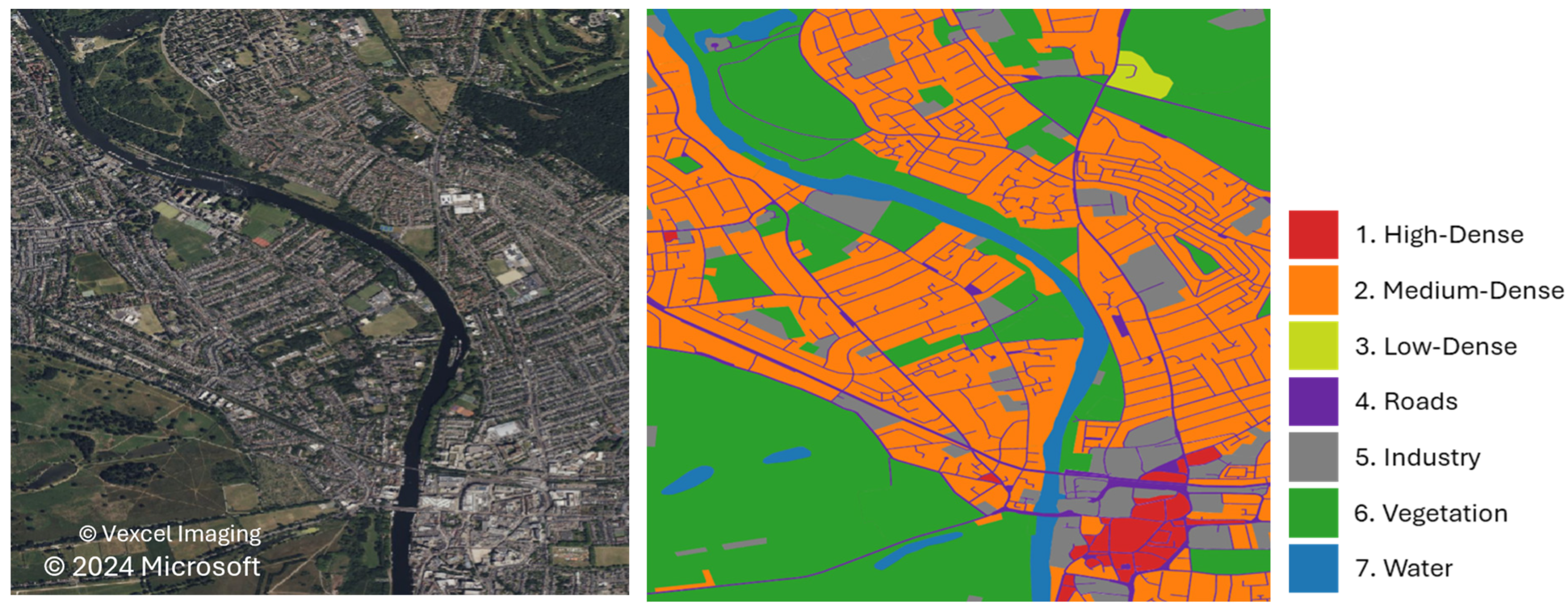
2.1. Datasets and Research Area

Developing a dataset with semantic labels for supervised learning is needed to classify urban density. Two different SAR sensors and two different urban locations were considered to evaluate the algorithm’s performance.
The study area covers part of London, Great Britain, and Warsaw, Poland. The two areas represent different urban systems with diverse topographical structures and various residential, commercial, and industrial buildings. These two large cities, with high diversity and a high probability of classes, were chosen deliberately. The imbalance in the area occupied by each category is due to the structure of the urban environment itself, in which some categories, such as residential zones, dominate over other categories, such as production zones. Figure 1 visualizes the two study areas.
SAR images from the following two sensors were collected: an X-band single-polarization image from ICEYE and a C-band dual-polarization image from Sentinel-1. The former has a higher spatial resolution but only a single polarization, VV (vertical transmit and vertical receive). In comparison, the latter has a lower spatial resolution but offers dual polarization, specifically VV and VH (vertical transmit and horizontal receive). The dates of the images were selected to be close to each other and cover the period without vegetation (i.e., autumn to winter seasons). For images from ICEYE, the spot extended area (SLEA) and strip map (SM) modes were used to capture the London and Warsaw areas, respectively. Both scenes were acquired using the interferometric wide (IW) mode on Sentinel-1. Table 1 describes the data’s properties. All SAR images were collected in the ground range detected (GRD) format, which is an amplitude format whereby images are multi-look processed and projected to the ground plane.

2.2. Urban Class Definition

Reference data from the UA were adapted for urban class definitions. The UA is a vector database of land use and land cover (LULC) data for various functional urban areas in European cities. It was created and is updated primarily through photo-interpretation methods using very-high-resolution (VHR) satellite optical imagery. The nomenclature is divided into 27 classes. A division’s minimum unit of area is 0.25 ha in urban areas and 1 ha in rural areas. The positional accuracy depends on the accuracy of the satellite imagery (2 m on average). The minimum distance between two mapping objects is 10 m. These parameters are essential not only for the processes of database creation and class recognition, but they also have consequences for the subsequent process of acquiring training data, as well as the automatic classification results on SAR imagery. The overall accuracy of the UA is 85% for urban classes (category 1) and 80% for other classes [38].
For residential areas, the UA distinguishes six classes, each with a unique identifier (ID) based on the urban density (Figure 2). The continuous urban fabric (ID 11100) comprises built-up areas and associated land, with soil sealing exceeding 80%. The predominant use is residential, encompassing downtown areas, city centers, and business districts that are also used for residential purposes. The discontinuous urban fabric is primarily composed of residential buildings, roads, and other areas with artificial surfaces, but it is further divided into the following subclasses: ID 11210, where the soil sealing is between 50% and 80%; ID 11220, where the soil sealing is between 30% and 50%, with vegetated areas, which are dominant; ID 11230, which is a discontinuous, low-density urban fabric, with soil sealing between 10% and 30%, where vegetated areas dominate but the land is not used for agriculture; ID 11240, which is very low density, with soil sealing less than 10%, such as residential houses with extensive gardens; and ID 11300, which has isolated structures with a residential component, such as small individual farms and related buildings, typically consisting of a few scattered or isolated houses.
The method of residential class aggregation is based on the area’s (polygon) percentage of occupation by development and gray infrastructure (i.e., sealed land). Hence, divisions are categorized into the following: high-, medium-, or low-density. Additional categories are based on the land cover and land use, such as vegetation and industrial land. These classes, as defined in this way, formed the basis for the thematic aggregation into Class 1, high-density (>80%); Class 2, medium-density (30–80%); and Class 3, low-density (<30%). Aggregation (Figure 2) was necessary to prepare the data for training and evaluating the supervised classification results.
Another category includes industrial, commercial, military, and transportation areas, which were also aggregated into the following two classes: roads (Class 4) or industrial and under-construction areas (Class 5). Classes with vegetation (e.g., IDs 14100, green urban areas; 14200, sports and recreational facilities; 20000, agricultural, semi-natural, and wetland areas; and 30000, forests) constituted a single common one — Class 6, vegetation. The final class is Class 7, water (ID 50000). This aggregation of areas with vegetation was conducted for the purpose of classifying and differentiating development classes rather than vegetation categories.
The 2018 version of the UA was used to create the datasets for London and Warsaw. The 27 LULC categories were aggregated into seven classes, with a focus on distinguishing dense urban areas. The definitions of all classes were carefully considered, and their combination results from both the function of each class and the potential for differentiation based on the data. Table 2 shows the class distributions for both study areas. Figure 3 illustrates an example of the aggregated UA classes.
Table 2 displays the class distributions for London and Warsaw. The most significant difference is between the high-density and medium-density classes. For Warsaw, most of the built-up areas were classified as high-density, whereas for London, the majority were classified as medium-density. The Warsaw study area features extensive railway infrastructure; consequently, the distribution of the roads class is greater than for London. Class 0 is “NoData”, labeling pixels with missing SAR or UA data, is ignored during training and evaluation.

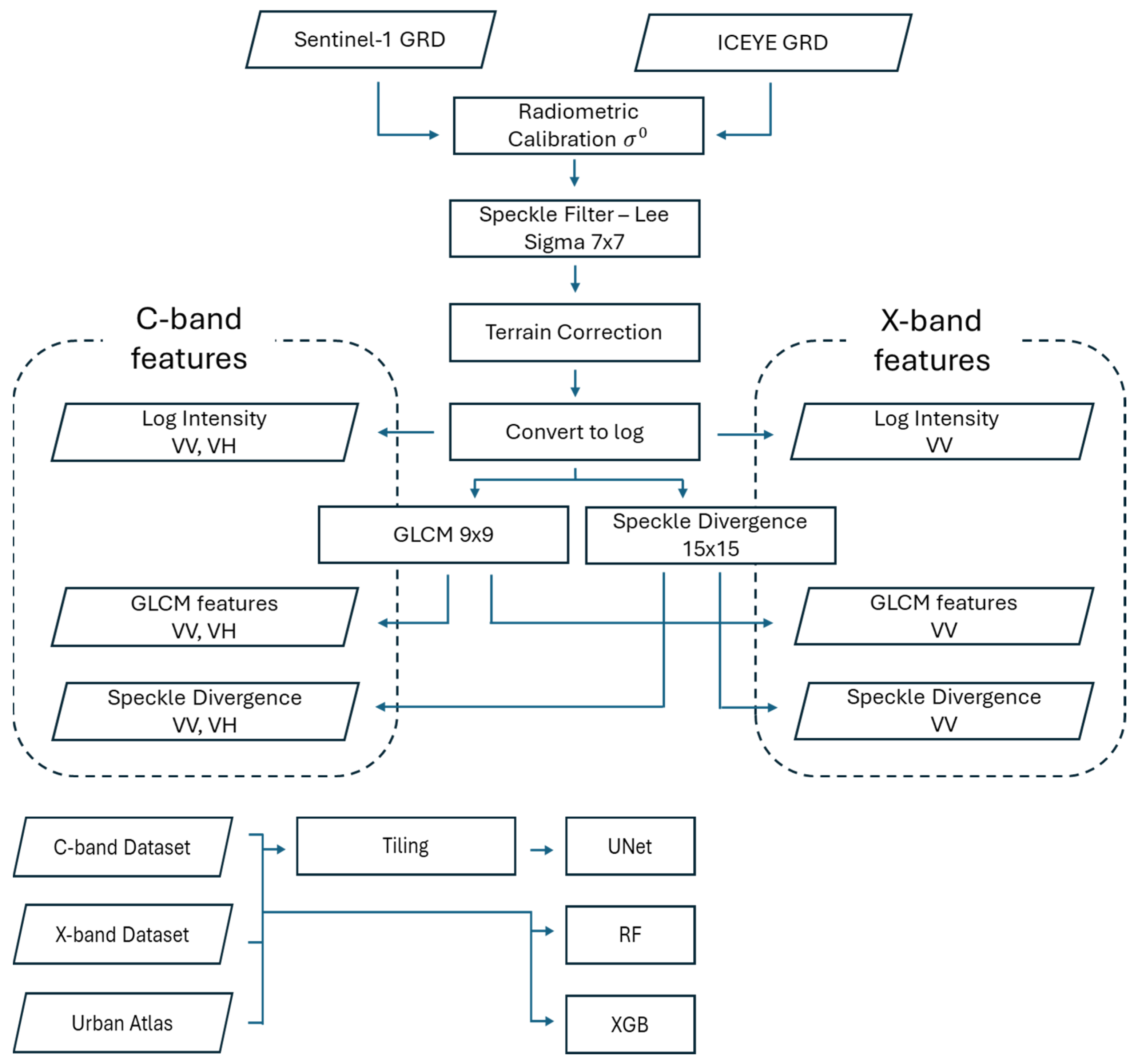
2.3. SAR Processing and Features

The preprocessing of each SAR image was similar to the process used in the Sentinel Application Platform (SNAP 9.0.0). It followed a standard processing pipeline for the GRD image format. It began with radiometric calibration, which converted the measured backscatter intensity into a normalized radar cross-section, taking into account the global incidence angle of the image and other sensor-specific characteristics. Using Lee sigma with a 7 × 7 window size, a speckle filter was applied to smooth out homogenous areas while preserving edges between different surfaces. Finally, terrain correction was applied to geocode the radar image into a coordinate system using a digital elevation model to correct for geometric distortions. The SAR preprocessing workflow is shown in Figure 4.
Three SAR features—log intensity, speckle divergence, and GLCM—were derived from the amplitude image to support its categorization into urban classes using UA labels.

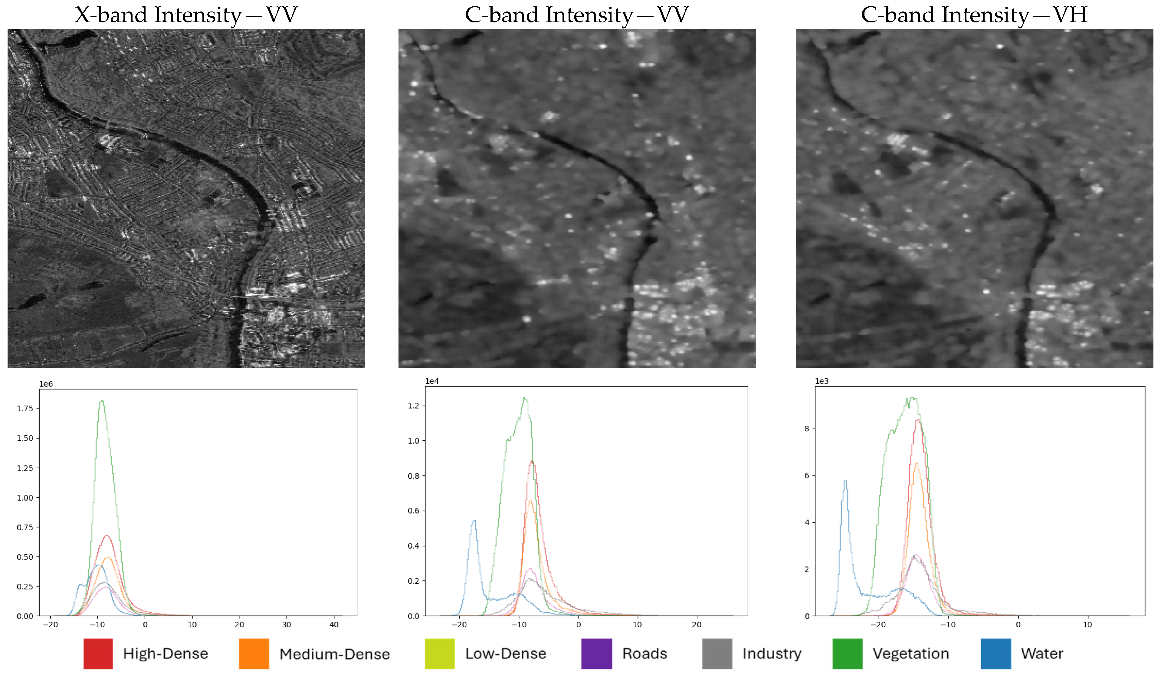
2.3.1. Log Intensity

Intensity refers to the mean amplitude of the recorded backscatter, which is influenced by the operating parameters of the radar system, such as the incidence angle and wavelength, as well as the characteristics of the ground targets, including their dielectric properties and roughness. The intensity image has an extensive dynamic range of values; therefore, the log of the intensity image was used.
Figure 5 shows additional details of an urban scene from an X-band SAR image compared to the C-band, in which edges representing road lines and building blocks are visible in the former. However, the class likelihood histogram for the X-band intensity shows overlaps among classes. This indicates there was difficulty in differentiating among the UA classes within this SAR feature. For the C-band SAR intensity, the water class was better distinguished from the other classes, exhibiting a low response in both VV and VH channels. The water class has an almost bimodal distribution due to the difference in backscatter from ponds and lakes compared to rivers. Other classes for both polarizations still had significant overlaps. Several building areas appear brighter in VV, most likely due to their orientation relative to the sensor.

2.3.2. Speckle Divergence

A combination of backscatter intensity and speckle divergence was used to delineate settlement areas with bright intensity and high speckle divergence [39]. This contrasts with natural areas, such as agricultural fields, water, or forests, which often exhibit relatively homogeneous textures, as shown in Figure 6.
Using SNAP, the speckle divergence was computed from the log intensity of the Sentinel-1 VV and VH polarizations, as well as the ICEYE VV polarization, with a window size of 15 × 15. The class histogram shows that all classes, except water, still have overlaps. Artificial structures, such as buildings, are depicted by bright points. However, there is no visible distinction between high- and medium-densities.

2.3.3. GLCM

Detailed structures of ground objects can be reflected in texture images. Buildings with regular arrangements and shapes show notable textural features in an image [40]. Textural features are extracted using GLCM based on the log intensity SAR image. The following five textural features were used, all calculated using a 9 × 9 window: energy, correlation, homogeneity, contrast, and variance. The homogeneity is illustrated in Figure 7, where similar pixels, such as water areas, have high values, while heterogeneous patterns, including buildings and infrastructure, have low values. In the X-band, the high-density class (red histogram) occupies lower values, indicating the class is slightly distinguishable from the others, which have a high degree of overlap. The water class in the co-pol VV is distinct, whereas in the cross-pol VH, all classes tend to occupy a narrow response range. This is consistent with other textural features in VH.

2.4. SAR Data Classification

In ML, semantic segmentation tasks involve assigning a semantic class to each pixel in an image. A supervised approach uses reference labels annotated at the pixel level to train a classifier to perform the task. This provides a higher resolution prediction than typical scene recognition from a patch of remote sensing images [9]. In this study, three algorithms were used for semantic segmentation. The following two algorithms are based on decision tree (DT): random forest (RF) and extreme gradient boosting (XGB). The third algorithm is based on a convolutional neural network (CNN).

2.4.1. Random Forest (RF)

RF is based on DT, an algorithm that recursively splits the input data. The branches represent the paths formed by repeated splits, while the leaves represent the final target class. DT has been widely used for land cover classification. It has fast computation, is easily interpretable, and software implementation is widely available [41]. However, DT struggles with complex and high-dimensional data. RF is an ensemble of many DTs, where the majority vote of all trees is used to assign a final class. This solves the weakness of a single DT, which can lead to non-optimal solutions and overfitting [15]. Each tree in an RF is trained on a random subset of the training data and using a random feature. This technique, known as bagging, ensures that each tree has less correlation, thereby improving the ensemble performance.
The RF implementation from cuML was used, which uses the graphics processing unit (GPU) to parallelize the training of each tree [42]. A hyperparameter search was conducted to identify the optimal parameters. The number of trees was 500, and the maximum depth of the nodes was 12.

2.4.2. Extreme Gradient Boosting (XGB)

XGB is an implementation of a scalable end-to-end ensemble ML algorithm based on DTs as the base learners [43]. The boosting technique aims to enhance the performance of previous trees during training. Like RF, a hyperparameter search was performed to determine the optimal parameters, with the following settings: 200 trees, a maximum depth of 6, and a learning rate of 0.15. Training was accelerated using the GPU.

2.4.3. U-Net (Unet)

The CNN and DL training pipeline was implemented using the PyTorch 2.0 framework [44] and the Segmentation Models library [45]. Adam [46] was the optimizer with a learning rate of 10 3 . A step-decaying scheduler modifies the learning rate with a decay factor of 0.95. A mini-batch size of 32 was used. Based on empirical findings, the reception field or input size of the CNN was chosen to be 256 by 256 pixels. The model was trained for 100 epochs to minimize the cross-entropy loss. We explored various well-studied models and concluded that the Unet [47] architecture, in combination with the ResNeSt26 [48] backbone, achieved the best performance with this dataset. For a deep learning model, the architecture refers to the connections between each layer in the network, while the backbone refers to the feature extraction part of the model.

2.5. Preprocessing

For RF and XGB, each pixel is considered a sample and was fitted into the GPU memory for training. For Unet, tiling was performed on the large SAR raster with a tile size of 512 by 512 pixels, with 128 pixels of overlaps for the ICEYE images and 256 pixels of overlaps for the Sentinel-1 images. As most SAR datasets have different spatial resolutions, the UA shapefiles were rasterized for each SAR dataset, generating label masks and distinct tiling areas. NoData regions in the label masks were set to 0, whereas the first label class started at 1 (high-density urban) and continued to 7 (water). During training, class 0 was ignored when computing the loss for the optimization and evaluating the metrics. Both the training area and evaluation area in Figure 1 were preprocessed similarly.

2.6. Evaluation

In this step, the evaluation area of each study area (indicated by the pink bounding boxes in Figure 1) was used to estimate the classification performance of the algorithms. In a binary classification, true positive (TP) indicates that a positive class was correctly predicted as positive, and true negative indicates a negative class was correctly predicted as negative. A false positive (FP) occurs when a negative class is incorrectly predicted as positive and vice versa for a false negative (FN). In multiclass classification tasks, the binary classification metrics for each class are computed, treating the target class as positive and the rest as negative.
Overall accuracy (OA) is the proportion of correctly classified pixels. It is intuitive to interpret it as how well the mode is performing. However, it might not report the performance across different classes effectively. It is computed by Equation (1), as follows:
O A = T P + T N T P + T N + F P + F N
The intersection over union (IoU) is a common metric for segmentation tasks, which is defined as the ratio of overlap between the predicted area and the true area, as shown in Equation (2), as follows:
I o U = y y ^ y y ^ = T P T P + F P + F N
In this multiclass segmentation task, a single pixel can belong to one of the seven classes. Therefore, the mean IoU (mIoU) from all classes is taken as the single metric for the model’s performance.
The F1-score is another common metric for segmentation tasks, more often used when there is an imbalance between positive and negative classes. It is the harmonic mean of the precision and recall and computed by Equation (3), as follows:
F 1 = 2 P r e c i s i o n × R e c a l l P r e c i s i o n + R e c a l l
Similarly, the F1-score for each class was computed, and the mean F1 (mF1) is reported.

3. Results

The following three algorithms were trained for segmenting the urban classes: RF and XGB, which are based on DTs, and Unet, which is based on a CNN. An initial hyperparameter optimization search was performed for each algorithm using only the log intensity feature to obtain a baseline model. Next, various combinations of SAR features were tested using the same training parameters as at baseline. Training and evaluation of the algorithms were conducted on an RTX A4000 GPU with 16 GB of video memory.

3.1. Algorithm and Feature Comparison

As shown in Table 3, the algorithms based on decision trees improved their prediction performance with more feature inputs. Their performances on the dual-polarimetry C-band SAR data were better than those for the X-band, which only has single-polarimetry capabilities. Since every pixel is considered a sample, DT-based algorithms rely on more features to better distinguish among classes [15]. Speckle divergence and GLCM utilize neighborhood filters that capture spatial context, which is why the combined features perform better compared to using only the log-intensity feature.
Meanwhile, additional features for the CNN-based algorithm tended to have a small impact on the performance. This is because the CNN can extract spatial features related to texture and edges inherently through convolutional filters [49]. Therefore, features derived from the log intensity might not provide new information. However, it was shown that adding speckle divergence yielded the highest mF1 for the X-band at 0.4960 (OA = 0.7843), while for the C-band, the highest mF1 was 0.4019 (OA = 0.7318) with the GLCM features. Compared to the C-band, the higher spatial detail from the X-band SAR data provided more spatial context for discriminating among classes, yielding better performance. A graphical comparison of the mIoU for each algorithm is shown in Figure 8.
The DT-based algorithms failed to classify the water and roads classes, as shown in Figure 9. Without balancing the training data, the complex backscatter patterns result in predictions dominated by the following three majority classes: medium-density, industrial, and vegetation. Their predictions appeared grainier, particularly visible in the X-band, which is caused by the salt-and-pepper-like texture from speckles in SAR. In Unet, the predictions are smoother due to the use of skip connections that retrieve better spatial details during the upscaling process in the decoder network [50]. Meanwhile, the DT-based algorithm resembles the raw appearance of objects in SAR based on their pixel values.
The deep convolutional layers enable the CNN to capture more complex spatial contexts within the boundaries of non-homogeneous texture [51,52]. These are highlighted by the white circles in Figure 9. On the top left circle, the label shows the continuous area of the water class. However, in the SAR image section, at the top, there appears to be some structure within the river, characterized by high backscatter, which was detected by the DT-based algorithms. The bottom right circle shows the industrial class next to a small, high-density class. As shown in the optical and SAR sections, at the bottom, the industrial and high-density classes tend to exhibit similar characteristics in SAR, characterized by a cluster of high backscatters resulting from layovers from high-rise buildings, complex rooftops, and building exteriors.
The confusion matrix for the Unet algorithm is shown in Figure 10. The minority classes were incorrectly predicted as major classes; specifically, the high-density area was misclassified as industrial, while the low-density area was misclassified as a vegetable class. It shows the model struggles to detect boundaries among classes since high-rise buildings in high-density areas look similar to industrial buildings. Because of its higher resolution, urban areas, roads, and industrial areas were classified more accurately in X-band. Meanwhile, both the X- and C-bands classified vegetation and water areas well.

3.2. Label Aggregation Comparison

In this section, we demonstrate the relationship between the number of classes and the classification performance. This is affected by the following two factors: a class’s appearance in SAR imagery and its distribution. The former impacts the discriminative features of each land class, which are used by the classifier. More classes that have negligible appearances would make it more difficult to discriminate. The latter affects the classifier’s bias, favoring classes with a greater distribution. Classifiers based on decision trees and neural networks perform effectively when the distribution of the response variables is balanced in the dataset [15].
We utilized the Unet model in this comparison. It was trained and evaluated using the seven-class nomenclature, with the fine urban density classes, and the five-class nomenclature, with the aggregated urban classes. As shown in Table 4, using the seven class labels yielded poor results for the finer classes. The five class labels exhibited a more discriminative appearance in the SAR data, resulting in improved performance. We investigate the use of class weights on the seven class labels. Class weights help reduce bias toward the majority class by assigning more importance to samples from the minority class.
For the London dataset, the majority of urban classes were dominated by the medium-density class. However, high-density and low-density classes accounted for only small percentages, leaving fewer samples with which to train. Because of this extreme class imbalance, using class weights did not significantly improve the classification of urban density classes in this study area. However, the detection of the road class improved, as indicated by the thicker purple edges in Figure 11.
For the Warsaw dataset, the distribution of the low-density class was even smaller than for London, resulting in no predictions of the class, regardless of whether class weights were used. The results are shown in Table 5. Class weights improved the performance on the X-band for the high-density class, which was the majority class here, and it also enhanced the minority classes, such as medium-density and roads. Despite having narrower highways than London, Warsaw has an extensive railway network, which leads to a higher percentage of the roads class, and it benefits from the use of class weights.
Similarly to London, when the problematic classes were combined as a single urban class, the mIoU increased significantly. The increase in IoU for the Industry class in the five-class model shows that it was easier to discriminate industrial areas when the urban classes were combined. However, the other classes did not improve significantly when the urban classes were combined, resulting in only a 0.04 increase in the OA score.

4. Discussion

4.1. Effects of SAR Sensors

Despite the availability of more details in X-band SAR, utilizing only the intensity values and textural features derived from it remains insufficient for distinguishing land use classes. This is mainly due to similar backscatter values for entirely different objects; for example, the specular reflectance of water has a similar low backscatter to shadows created by the blind spots of high-rise buildings. Several studies have pointed out the limitations of single- or dual-polarization SAR for classification [53,54]. The Unet algorithm performed better than the DT-based algorithms, since it learns the relationship between labels and the underlying radar signature iteratively. Neural networks consider not only spectral and textural features but also geometric and multiscale neighboring information, similar to what a human analyst would recognize.
As with any object detection using remote sensing, there is a trade-off between spatial resolution and the object’s size. Large ponds and parks are delineated better in Sentinel-1’s C-band image, which has a lower resolution. Moreover, the finer details and shorter wavelength SAR mean that an X-band image is more sensitive to minor surface roughness, such as the surface of water, which appears to have a non-homogeneous texture due to backscatter from small ripples. The trade-off is that finer details, such as smaller objects like residential buildings and roads, are still observable. In contrast, in the C-band, only larger features, like highways or major rail stations, can be visible.

4.2. Reliability of Urban Atlas

Objects labeled in the UA database are affected by their patterns of land use distribution and the organization of city blocks. This labeling process, which follows the function of the land, complicates the task of classifying different physical appearances as the same class, for example, a large object with non-homogeneous patterns, such as an airport. The airport’s connected infrastructure, such as terminals, bus stations, and hotels, is represented by bright edges, while a grainy texture represents the surrounding vegetation area. Classifying these complex and different patterns as the same class will be difficult for any algorithm. A similar problem occurs for the class “industrial, commercial, public, military”, in which artificial surfaces cover at least 30%, and buildings or artificial structures of non-residential use occupy greater than 50%. This refers not only to land cover but to its function, introducing subjectivity into the delineation of class polygons and making it difficult to use this database for the training and evaluation stages of SAR classified imagery.
Additionally, we observed discrepancies in the classification of high- and medium-density urban areas between London and Warsaw. In Warsaw, most polygons classified as high-density do not meet the criterion and should be reclassified as medium-density, hence, the approx. 10%weaker results for Warsaw, independent of the sensor (S-1 or ICEYE). The use of the UA for reference labels to classify the building density is limited by the consistency of the labelers. To prevent subjectivity and the replication of errors by classifiers trained on this dataset, standardization of the interpretation and plotting of class contours is required [55].

4.3. Accuracy of the Results

The tests performed showed an overall accuracy (OA) of an average level. For London, the best results were 79% for the X-band and 73% for the C-band datasets. For Warsaw, the best results were 68% for the X-band and 64% for the C-band datasets. It is worthwhile to compare the results achieved with those reported in the literature.
Zhu et al. [12] tested the classification of urban land cover types, including low-density residential, high-density residential, and commercial/industrial areas, based on PALSAR and optical data. The inclusion of SAR data improved the overall classification by 1.1%. Relatively high producer’s (81%) and user’s (75%) accuracies were observed for high-density residential areas. In comparison, the producer’s and user’s accuracies for the low-density residential and commercial or industrial areas were below average (approximately 70% or less). The low-density residential class was frequently misclassified as forest. Commercial or industrial areas were sometimes misclassified as high-density residential [40]. Similar results were achieved with K-means classification, with a 0.32-0.45 level for the MIoU using UAVSAR data for three different urban areas [56]. The results of Corbane [57] show that the SAR backscatter from an urban environment is highly dependent on the radar frequency, polarization, and viewing geometry. Therefore, SAR imagery allows for the detection of urban features in a complementary way. Still, it can also become blind toward other buildings and structures depending on the viewing geometry, incidence angle, and urban fabric [57,58].
Other researchers have also pointed out the challenges in urban area classification, particularly in terms of the complexity of landscapes and difficulty in distinguishing among built-up classes. Some are supported by multi-source data from SAR and optical sensors to enhance the quality of the results, focusing on urban impervious surfaces (UIS) rather than specific urban classes. The research in [59] presents a comparison of two ensemble machine learning classifiers, RF and XGB, using an integration of optical and SAR features. Sentinel-1 and Landsat 8 datasets were used with SAR textures and enhanced modified indices to extract features for the year 2023. The study focused on three significant East Asian cities with diverse urban dynamics—Jakarta, Manila, and Seoul—for UIS extraction. The results showed an overall accuracy of 81% for the UIS classification using XGB and 77% with RF when classifying land cover into the following four major classes: water, vegetation, bare soil, and urban impervious areas. Still, all of the results indicate poor separability between the bare soil class and ground truth data [59].
An ensemble machine learning approach using optical–SAR datasets was implemented to enhance the accuracy of UIS mapping [60]. Four algorithms, including AdaBoost, gradient boost, XGB, and RF, were tested, achieving a classification accuracy of 92% and consistently performing across 32 cities. Regarding the UIS accuracy and predictive power, XGB outperformed the other classifiers. A comparative analysis with three datasets, ESA World Cover, ESRI Land Cover, and Dynamic World (DW), was also performed. The proposed UIS model outperformed renowned global datasets, followed by DW at 83%, ESA at 86%, and ESRI at 82% [60].
In the case of Morocco [42], RF classification was used to detect diverse built-up structures. The outcomes revealed that the combination of Sentinel-1 and Sentinel-2 data resulted in a kappa value of 0.87, followed by the SAR composite. The lowest accuracy value was obtained with the optical composite [61]. In another study in an Indian city, fully polarimetric L-band ALOS-2 SAR data were used for the rapid identification of urban regions. The results of the classification with two classes, urban and non-urban, indicate that the support vector machine (SVM) outperformed the Wishart supervised classification algorithm [62]. Another method, MCANet, is a multimodal cross-attention network, i.e., a joint semantic segmentation framework combining optical and SAR images for land use classification. The classification accuracy of this approach was approximately 5% higher than that of only optic-image-based approaches [11].
Accurate extraction of urban classes from SAR data remains a challenge, especially for cities with high heterogeneity. Modern techniques yield promising results at the global or regional scale when using aggregated building classes, but the accuracy decreases at the city scale when employing detailed urban classes. Nevertheless, researchers note that these results can serve to support urban monitoring and planning.

5. Conclusions

In this study, we examined the challenges related to urban land segmentation, with a focus on building density, using SAR images. A novel dataset based on the UA database was created for this supervised segmentation task. Seven urban classes were aggregated from the UA labels, which consisted of three building density classes. Two different SAR sensors were considered: a single-polarization X-band sensor and a dual-polarization C-band sensor. We extracted the following three features from the SAR amplitude image: log intensity, speckle divergence, and GLCM. The class likelihood histogram indicates low class separability from the features, particularly among the three building density classes.
Using the dataset, we analyzed the performances of three supervised algorithms, namely, RF, XGB, and Unet. The DT-based algorithms improved with more neighborhood image features and smoother texture from the lower resolution C-band SAR, yielding the best OA of 73% with all combined features. In the high-resolution X-band, the DT-based algorithms were sensitive to the class distribution and speckle noise, resulting in poor performances. Meanwhile, the CNN-based Unet could utilize the high details of the X-band to recognize objects from small classes, such as roads and buildings, and it yielded the best performance at 78% OA with the combined features of log intensity and speckle divergence. Overall, the robustness of the convolutional layers in extracting neighborhood features reduces the need for additional derived features. Moreover, class weights can be applied to improve the detection of minority classes resulting from the natural imbalance of the class distribution in urban areas. The use of the public UA database with SAR images for urban land classification is limited. A stricter labeling process is needed to improve the consistency of the trained classifier and reduce label bias.

Author Contributions

Conceptualization, J.P.-K.; methodology, J.P.-K. and S.W.; validation, J.P.-K. and S.W.; formal analysis, J.P.-K. and S.W.; investigation, J.P.-K. and S.W.; writing—original draft preparation, J.P.-K.; writing—review and editing, as well as visualization, J.P.-K. and S.W.; supervision, project administration, and funding acquisition, J.P.-K. All authors have read and agreed to the published version of the manuscript.

Funding

This paper was co-financed under the research grant of the Warsaw University of Technology supporting the scientific activity in the discipline of Civil Engineering, Geodesy, and Transport. The authors thank ICEYE and ESA for making SAR data available for free via an open-access platform under the ESA Earth Observation Proposal Project, PP0093612/2023.

Data Availability Statement

The original contributions presented in this study are included in the article. Further inquiries can be directed to the corresponding author.

Acknowledgments

We acknowledge that open access to software, tools, and libraries made the study possible.

Conflicts of Interest

The authors declare no conflicts of interest. The funders had no role in the design of the study, the collection, analysis, or interpretation of data, the writing of the manuscript, or the decision to publish the results.

References

  1. GHSL. Global Human Settlement—GHSL Homepage—European Commission. Available online: https://human-settlement.emergency.copernicus.eu/ (accessed on 28 June 2024).
  2. European Commission, Joint Research Centre. GHSL Data Package 2023; Publications Office: Luxembourg, 2023; Available online: https://data.europa.eu/doi/10.2760/098587 (accessed on 26 July 2024).
  3. Pesaresi, M. GHS-BUILT-S R2023A—GHS Built-up Surface Grid, Derived from Sentinel2 Composite and Landsat, Multitemporal (1975–2030); European Commission, Joint Research Centre (JRC): Brussels, Belgium, 2023. [Google Scholar] [CrossRef]
  4. Florczyk, A.; Corbane, C.; Schiavina, M.; Pesaresi, M.; Freire, S.; Sabo, F.; Tommasi, P.; Airaghi, D.; Ehrlich, D.; Melchiorri, M.; et al. GHS-UCDB R2019A—GHS Urban Centre Database 2015, Multitemporal and Multidimensional Attributes; European Commission, Joint Research Centre (JRC): Brussels, Belgium, 2019. [Google Scholar] [CrossRef]
  5. Denis, M. Selected Issues Regarding Small Compact City—Advantages And Disadvantages. piF 2018, 2018, 151–162. [Google Scholar] [CrossRef]
  6. Salem, A. Determining an Adequate Population Density to Achieve Sustainable Development and Quality of Life. In The Role of Design, Construction, and Real Estate in Advancing the Sustainable Development Goals; Walker, T., Cucuzzella, C., Goubran, S., Geith, R., Eds.; Sustainable Development Goals Series; Springer International Publishing: Cham, Switzerland, 2023; pp. 105–128. [Google Scholar] [CrossRef]
  7. Denis, M.; Cysek-Pawlak, M.M.; Krzysztofik, S.; Majewska, A. Sustainable and vibrant cities. Opportunities and threats to the development of Polish cities. Cities 2021, 109, 103014. [Google Scholar] [CrossRef]
  8. Batty, M. The Size, Scale, and Shape of Cities. Science 2008, 319, 769–771. [Google Scholar] [CrossRef]
  9. Pluto-Kossakowska, J. Automatic detection of grey infrastructure based on vhr image. Int. Arch. Photogramm. Remote Sens. Spat. Inf. Sci. 2020, XLIII-B3-2020, 181–187. [Google Scholar] [CrossRef]
  10. De Sousa, F.L. Are smallsats taking over bigsats for land Earth observation? Acta Astronaut. 2023, 213, 455–463. [Google Scholar] [CrossRef]
  11. Li, X.; Zhang, G.; Cui, H.; Hou, S.; Wang, S.; Li, X.; Chen, Y.; Li, Z.; Zhang, L. MCANet: A joint semantic segmentation framework of optical and SAR images for land use classification. Int. J. Appl. Earth Obs. Geoinf. 2022, 106, 102638. [Google Scholar] [CrossRef]
  12. Zhu, Z.; Woodcock, C.E.; Rogan, J.; Kellndorfer, J. Assessment of spectral, polarimetric, temporal, and spatial dimensions for urban and peri-urban land cover classification using Landsat and SAR data. Remote Sens. Environ. 2012, 117, 72–82. [Google Scholar] [CrossRef]
  13. Bi, H.; Xu, L.; Cao, X.; Xue, Y.; Xu, Z. Polarimetric SAR Image Semantic Segmentation With 3D Discrete Wavelet Transform and Markov Random Field. IEEE Trans. Image Process. 2020, 29, 6601–6614. [Google Scholar] [CrossRef]
  14. Qu, J.; Qiu, X.; Wang, W.; Wang, Z.; Lei, B.; Ding, C. A Comparative Study on Classification Features between High-Resolution and Polarimetric SAR Images through Unsupervised Classification Methods. Remote Sens. 2022, 14, 1412. [Google Scholar] [CrossRef]
  15. Maxwell, A.E.; Warner, T.A.; Fang, F. Implementation of machine-learning classification in remote sensing: An applied review. Int. J. Remote Sens. 2018, 39, 2784–2817. [Google Scholar] [CrossRef]
  16. Mohammadimanesh, F.; Salehi, B.; Mahdianpari, M.; Gill, E.; Molinier, M. A new fully convolutional neural network for semantic segmentation of polarimetric SAR imagery in complex land cover ecosystem. ISPRS J. Photogramm. Remote Sens. 2019, 151, 223–236. [Google Scholar] [CrossRef]
  17. Hall-Beyer, M. Practical guidelines for choosing GLCM textures to use in landscape classification tasks over a range of moderate spatial scales. Int. J. Remote Sens. 2017, 38, 1312–1338. [Google Scholar] [CrossRef]
  18. Dell’Acqua, F.; Gamba, P. Texture-based characterization of urban environments on satellite SAR images. IEEE Trans. Geosci. Remote Sens. 2003, 41, 153–159. [Google Scholar] [CrossRef]
  19. Holobâcă, I.-H.; Ivan, K.; Mircea, A. Extracting built-up areas from Sentinel-1 imagery using land-cover classification and texture analysis. Int. J. Remote Sens. 2019, 40, 8054–8069. [Google Scholar] [CrossRef]
  20. Kupidura, P.; Uwarowa, I. The comparison of GLCM and granulometry for distinction of different classes of urban area. In Proceedings of the 2017 Joint Urban Remote Sensing Event (JURSE), Dubai, United Arab Emirates, 6–8 March 2017; IEEE: Piscataway, NJ, USA, 2017; pp. 1–4. [Google Scholar] [CrossRef]
  21. Molch, K.; Radar Earth Observation Imagery for Urban Area Characterisation. JRC Publications Repository. Available online: https://publications.jrc.ec.europa.eu/repository/handle/JRC50451 (accessed on 28 June 2024).
  22. Goodman, J.W. Some fundamental properties of speckle*. J. Opt. Soc. Am. 1976, 66, 1145. [Google Scholar] [CrossRef]
  23. Eckardt, R.; Urbazaev, M.; Salepci, N.; Schmullius, C.; Woodhouse, I.; Stewart, C. “MOOC on SAR: Echoes in Space,” Eo Science for Society. Available online: https://eo4society.esa.int/resources/echoes-in-space/ (accessed on 28 June 2024).
  24. Snitkowska, E. Analiza Tekstur w Obrazach Cyfrowych i jej Zastosowanie do Obrazów Angiograficznych. Warszawa, 2004. Available online: https://www.ia.pw.edu.pl/~wkasprza/PAP/PhDEwaSnitkowska.pdf (accessed on 28 June 2024).
  25. Dell’Acqua, F.; Gamba, P.; Trianni, G. Semi-automatic choice of scale-dependent features for satellite SAR image classification. Pattern Recognit. Lett. 2006, 27, 244–251. [Google Scholar] [CrossRef]
  26. Kamusoko, C. Optical and SAR Remote Sensing of Urban Areas: A Practical Guide; Springer geography; Springer: Singapore, 2022. [Google Scholar]
  27. Huang, X.; Zhang, T. Morphological Building Index (MBI) and Its Applications to Urban Areas. In Urban Remote Sensing, 2nd ed.; CRC Press: Boca Raton, FL, USA, 2018; pp. 33–49. [Google Scholar]
  28. Hall-Beyer, M. GLCM Texture: A Tutorial v. 3.0 March 2017. 2017. Available online: http://hdl.handle.net/1880/51900 (accessed on 28 June 2024).
  29. Haralick, R.M.; Shanmugam, K.; Dinstein, I. Textural Features for Image Classification. IEEE Trans. Syst. Man Cybern. 1973, SMC-3, 610–621. [Google Scholar] [CrossRef]
  30. Esch, T.; Roth, A. Semi-Automated Classification of Urban Areas by Means of High Resolution Radar Data. 2004. Available online: https://www.isprs.org/proceedings/xxxv/congress/comm7/papers/93.pdf (accessed on 28 June 2024).
  31. Semenzato, A.; Pappalardo, S.E.; Codato, D.; Trivelloni, U.; De Zorzi, S.; Ferrari, S.; De Marchi, M.; Massironi, M. Mapping and Monitoring Urban Environment through Sentinel-1 SAR Data: A Case Study in the Veneto Region (Italy). IJGI 2020, 9, 375. [Google Scholar] [CrossRef]
  32. Stasolla, M.; Gamba, P. Spatial Indexes for the Extraction of Formal and Informal Human Settlements From High-Resolution SAR Images. IEEE J. Sel. Top. Appl. Earth Obs. Remote Sens. 2008, 1, 98–106. [Google Scholar] [CrossRef]
  33. Soergel, U. (Ed.) Radar remote sensing of urban areas. In Remote Sensing and Digital Image Processing; Springer: Dordrecht, The Netherlands; New York, NY, USA, 2010. [Google Scholar]
  34. Wangiyana, S.; Samczyński, P.; Gromek, A. Data Augmentation for Building Footprint Segmentation in SAR Images: An Empirical Study. Remote Sens. 2022, 14, 2012. [Google Scholar] [CrossRef]
  35. Bruzzone, L.; Marconcini, M.; Wegmuller, U.; Wiesmann, A. An advanced system for the automatic classification of multitemporal SAR images. IEEE Trans. Geosci. Remote Sens. 2004, 42, 1321–1334. [Google Scholar] [CrossRef]
  36. Kupidura, P. The Comparison of Different Methods of Texture Analysis for Their Efficacy for Land Use Classification in Satellite Imagery. Remote Sens. 2019, 11, 1233. [Google Scholar] [CrossRef]
  37. Su, W.; Li, J.; Chen, Y.; Liu, Z.; Zhang, J.; Low, T.M.; Suppiah, I.; Hashim, S.A.M. Textural and local spatial statistics for the object-oriented classification of urban areas using high resolution imagery. Int. J. Remote Sens. 2008, 29, 3105–3117. [Google Scholar] [CrossRef]
  38. Urban Atlas, G. Urban Atlas—Copernicus Land Monitoring Service. Available online: https://land.copernicus.eu/en/products/urban-atlas (accessed on 28 June 2024).
  39. Thiel, M.; Esch, T.; Schenk, A. Object-Oriented Detection Of Urban Areas From TerraSAR-X Data. In Proceedings of the ISPRS 2008 Congress, Beijing, China, 3–11 July 2008; Volume XXXVII Part B8. [Google Scholar]
  40. Zhai, W.; Shen, H.; Huang, C.; Pei, W. Fusion of polarimetric and texture information for urban building extraction from fully polarimetric SAR imagery. Remote Sens. Lett. 2016, 7, 31–40. [Google Scholar] [CrossRef]
  41. Pal, M.; Mather, P.M. An assessment of the effectiveness of decision tree methods for land cover classification. Remote Sens. Environ. 2003, 86, 554–565. [Google Scholar] [CrossRef]
  42. Raschka, S.; Patterson, J.; Nolet, C. Machine Learning in Python: Main developments and technology trends in data science, machine learning, and artificial intelligence. arXiv 2020. [Google Scholar] [CrossRef]
  43. Chen, T.; Guestrin, C. XGBoost: A Scalable Tree Boosting System. In Proceedings of the 22nd ACM SIGKDD International Conference on Knowledge Discovery and Data Mining, San Francisco, CA, USA, 13–17 August 2016; ACM: New York, NY, USA, 2016; pp. 785–794. [Google Scholar] [CrossRef]
  44. Paszke, A.; Gross, S.; Massa, F.; Lerer, A.; Bradbury, J.; Chanan, G.; Killeen, T.; Lin, Z.; Gimelshein, N.; Antiga, L.; et al. PyTorch: An Imperative Style, High-Performance Deep Learning Library. arXiv 2019, arXiv:1912.01703. [Google Scholar] [CrossRef]
  45. Iakubovskii. Qubvel/Segmentation_Models.Pytorch. Available online: https://github.com/qubvel/segmentation_models.pytorch (accessed on 9 September 2023).
  46. Kingma, D.P.; Ba, J. Adam: A Method for Stochastic Optimization. arXiv 2014. [Google Scholar] [CrossRef]
  47. Ronneberger, O.; Fischer, P.; Brox, T. U-Net: Convolutional Networks for Biomedical Image Segmentation. arXiv 2015. [Google Scholar] [CrossRef]
  48. Zhang, H.; Wu, C.; Zhang, Z.; Zhu, Y.; Lin, H.; Zhang, Z.; Sun, Y.; He, T.; Mueller, J.; Manmatha, R.; et al. ResNeSt: Split-Attention Networks. arXiv 2020, arXiv:2004.08955. [Google Scholar]
  49. Krizhevsky, A.; Sutskever, I.; Hinton, G.E. ImageNet classification with deep convolutional neural networks. Commun. ACM 2017, 60, 84–90. [Google Scholar] [CrossRef]
  50. Seferbekov, S.S.; Iglovikov, V.I.; Buslaev, A.V.; Shvets, A.A. Feature Pyramid Network for Multi-Class Land Segmentation. arXiv 2018. [Google Scholar] [CrossRef]
  51. Tan, M.; Le, Q.V. EfficientNet: Rethinking Model Scaling for Convolutional Neural Networks. arXiv 2019. [Google Scholar] [CrossRef]
  52. Alzubaidi, L.; Zhang, J.; Humaidi, A.J.; Al-Dujaili, A.; Duan, Y.; Al-Shamma, O.; Santamaría, J.; Fadhel, M.A.; Al-Amidie, M.; Farhan, L. Review of deep learning: Concepts, CNN architectures, challenges, applications, future directions. J. Big Data 2021, 8, 53. [Google Scholar] [CrossRef]
  53. Ji, K.; Wu, Y. Scattering Mechanism Extraction by a Modified Cloude-Pottier Decomposition for Dual Polarization SAR. Remote Sens. 2015, 7, 7447–7470. [Google Scholar] [CrossRef]
  54. Bai, Y.; Adriano, B.; Mas, E.; Koshimura, S. Building Damage Assessment in the 2015 Gorkha, Nepal, Earthquake Using Only Post-Event Dual Polarization Synthetic Aperture Radar Imagery. Earthq. Spectra 2017, 33, 185–195. [Google Scholar] [CrossRef]
  55. Jiang, H.; Nachum, O. Identifying and Correcting Label Bias in Machine Learning. arXiv 2019. [Google Scholar] [CrossRef]
  56. Sarkar, S.; Halder, T.; Poddar, V.; Gayen, R.K.; Ray, A.M.; Chakravarty, D. A Novel Approach for Urban Unsupervised Segmentation Classification in SAR Polarimetry. In Proceedings of the 2021 2nd International Conference on Range Technology (ICORT), Chandipur, Balasore, India, 5–6 August 2021; IEEE: Piscataway, NJ, USA, 2021; pp. 1–5. [Google Scholar] [CrossRef]
  57. Corbane, C.; Faure, J.-F.; Baghdadi, N.; Villeneuve, N.; Petit, M. Rapid Urban Mapping Using SAR/Optical Imagery Synergy. Sensors 2008, 8, 7125–7143. [Google Scholar] [CrossRef] [PubMed]
  58. Corbane, C.; Sabo, F. European Settlement Map from Copernicus Very High Resolution Data for Reference Year 2015, Public Release 2019; European Commission, Joint Research Centre (JRC): Brussels, Belgium, 2019. [Google Scholar] [CrossRef]
  59. Shao, Z.; Ahmad, M.N.; Javed, A. Comparison of Random Forest and XGBoost Classifiers Using Integrated Optical and SAR Features for Mapping Urban Impervious Surface. Remote Sens. 2024, 16, 665. [Google Scholar] [CrossRef]
  60. Ahmad, M.N.; Shao, Z.; Xiao, X.; Fu, P.; Javed, A.; Ara, I. A novel ensemble learning approach to extract urban impervious surface based on machine learning algorithms using SAR and optical data. Int. J. Appl. Earth Obs. Geoinf. 2024, 132, 104013. [Google Scholar] [CrossRef]
  61. Tayi, S.; Radoine, H. Mapping built-up area: Combining Radar and Optical Imagery using Google Earth Engine. In Proceedings of the 2023 Joint Urban Remote Sensing Event (JURSE), Heraklion, Greece, 17–19 May 2023; IEEE: Piscataway, NJ, USA, 2023; pp. 1–4. [Google Scholar] [CrossRef]
  62. Kanade, D.S.; Vanama, V.S.K.; Shitole, S. Urban area classification with quad-pol L-band ALOS-2 SAR data: A case of Chennai city, India. In Proceedings of the 2020 IEEE India Geoscience and Remote Sensing Symposium (InGARSS), Ahmedabad, India, 1–4 December 2020; IEEE: Piscataway, NJ, USA, 2020; pp. 58–61. [Google Scholar] [CrossRef]
Figure 1. The study areas are London, UK (left), and Warsaw, PL (right). The blue polygons represent the training areas, while the pink polygons represent the evaluation areas. London’s training and evaluation areas are 188 km2 and 65 km2, respectively, while Warsaw’s are 202 km2 and 65 km2, respectively, as based on ESRI.
Remotesensing 17 01606 g001
Figure 2. Aggregation scheme for urban area classification with the UA codes.
Remotesensing 17 01606 g002
Figure 3. A section of the scene for London comparing the SAR features: (right) optical image from Bing Maps; (left) corresponding UA labels with a colored legend aggregated into seven classes.
Remotesensing 17 01606 g003
Figure 4. The preprocessing workflow in SNAP for both Sentinel-1 C-band and ICEYE X-band images. The bottom image shows the data processing workflow for the three algorithms.
Remotesensing 17 01606 g004
Figure 5. SAR intensity features and the class likelihood histogram for X-band (ICEYE) and C-band (Sentinel-1) images.
Remotesensing 17 01606 g005
Figure 6. Examples of X-band (ICEYE) and C-band (S-1) speckle divergence images with histograms of the urban classes.
Remotesensing 17 01606 g006
Figure 7. An example of a textural feature is homogeneity, calculated using the GLCM for X-band (ICEYE) and C-band (Sentinel-1) images.
Remotesensing 17 01606 g007
Figure 8. Comparison between algorithms and features using mIoU. X stands for the X-band SAR image from ICEYE, while C stands for the C-band dual-polarimetry SAR image from Sentinel-1; the mIoU metric ranges between 0.0 and 1.0, where 1.0 indicates the highest value.
Remotesensing 17 01606 g008
Figure 9. Visual comparison of the predictions from each algorithm using their optimal feature combination. On the right is the reference label from the UA, along with sections of optical and SAR images of two interesting areas, as highlighted by white circles.
Remotesensing 17 01606 g009
Figure 10. Confusion matrix for Unet on the London study area. On the right color scale.
Remotesensing 17 01606 g010
Figure 11. Comparison of the use of class weights in the London study area. White circles highlight two interesting areas.
Remotesensing 17 01606 g011
Table 1. SAR product specifications used in the study.
ParameterLondonWarsaw
Imaging ModeICEYE SLEASentinel-1 IWICEYE SMSentinel-1 IW
Band (frequency GHz)X (9.6)C (5.4)X (9.6)C (5.4)
Input formatGRDGRDGRDGRD
PolarizationVVVV, VHVVVV, VH
OrbitAscendingDescendingDescendingDescending
Look sideRightRightRightRight
Ground resolution (m)0.5 × 0.510.0 × 10.02.5 × 2.510.0 × 10.0
Date20-12-202118-12-202118-09-201919-09-2019
Area (km2)253 253267267
Table 2. Class distribution of UA labels for both research areas.
Class IDClass NamesLondon (%)Warsaw (%)
0Background (NoData)3.225.59
1High-Density0.3426.53
2Medium-Density32.756.12
3Low-Density0.260.21
4Roads7.4910.35
5Industry17.2418.43
6Vegetation33.5530.47
7Water5.142.31
Table 3. Results from the three algorithms and a combination of features were trained and evaluated on the London dataset. The features were int (log intensity), spk (speckle divergence), and glcm (combined features from GLCM). The metrics range from 0.0 to 1.0, where 1.0 indicates the highest value. The best results are in bold.
AlgorithmFeaturesX-BandC-Band
intspkglcmOAmIoUmF1OAmIoUmF1
RF 0.40040.09810.15290.55130.21340.2977
0.52630.13560.19170.62400.26050.3493
0.53170.14260.20010.63590.26120.3473
0.55230.15070.20780.65190.27510.3623
XGB 0.39880.09800.15290.60750.23740.3236
0.53930.14540.20270.62850.26230.3506
0.53470.14660.20760.64280.26480.3504
0.55530.15460.21510.66040.28000.3663
Unet 0.77010.35850.44830.72330.31820.3971
0.78430.39260.49600.71670.31400.3934
0.77180.37080.47150.73180.32140.4019
0.78230.37100.46600.71750.31340.3939
Table 4. Results from the Unet algorithm with class weights and a 5-class nomenclature for London.
BandLabelsIoUmIoUOA
Urban DensityRoadIndustryVegetationWater
HighMediumLow
X-band7c0.09410.72950.00000.17440.34300.77130.63630.39260.7843
7c weighted0.07220.66750.01110.18630.32270.74040.55120.36450.7442
5c0.72030.16540.33550.76570.61580.52060.7879
C-band7c0.00000.61460.00000.00000.27830.68160.67540.32140.7318
7c weighted0.21470.55220.00000.06670.20210.65480.65340.33490.6737
5c0.62050.00140.26800.68110.65280.44480.7349
Table 5. Results from the Unet algorithm with class weights and with a 5-class nomenclature for Warsaw.
BandLabelsIoUmIoUOA
Urban FabricRoadIndustryVegetationWater
HighMediumLow
X-band7c0.49320.02680.00000.19930.32690.66710.75650.35280.6287
7c weighted0.51540.06710.00000.24340.35410.66140.71680.36540.6447
5c0.56190.22890.36910.62860.77060.51180.6811
C-band7c0.47220.06290.00000.01020.32500.61780.67700.30930.6004
7c weighted0.42890.09160.00000.09430.29450.57000.66800.30680.5365
5c0.51730.06920.30350.59380.68520.43380.6386
Disclaimer/Publisher’s Note: The statements, opinions and data contained in all publications are solely those of the individual author(s) and contributor(s) and not of MDPI and/or the editor(s). MDPI and/or the editor(s) disclaim responsibility for any injury to people or property resulting from any ideas, methods, instructions or products referred to in the content.

