Article

Mapping Forest Aboveground Biomass with Phenological Information Extracted from Remote Sensing Images in Subtropical Evergreen Broadleaf Forests

1
Research Center of Forestry Remote Sensing and Information Engineering, Central South University of Forestry and Technology, Changsha 410004, China
2
Key Laboratory of Forestry Remote Sensing Based Big Data and Ecological Security for Hunan Province, Changsha 410004, China
3
Key Laboratory of State Forestry Administration on Forest Resources Management and Monitoring in Southern Area, Changsha 410004, China
4
State Key Laboratory of Black Soils Conservation and Utilization, Northeast Institute of Geography and Agroecology, Chinese Academy of Sciences, Changchun 130102, China
*
Author to whom correspondence should be addressed.
Remote Sens. 2025, 17(9), 1599; https://doi.org/10.3390/rs17091599
Submission received: 11 February 2025 / Revised: 18 April 2025 / Accepted: 24 April 2025 / Published: 30 April 2025

Abstract

:
Forest aboveground biomass (AGB) serves as a crucial quantitative indicator that reflects the carbon sequestration capacity of forests, and accurately mapping AGB is pivotal for assessing forest ecosystem stability. However, mapping AGB in subtropical evergreen broadleaf forests in southern China presents challenges due to their complex canopy structure, stand heterogeneity, and spectral signal saturation. The phenological features reflecting seasonal vegetation dynamics are conducive to over-coming these challenges. By analyzing differential spectral reflectance patterns during the non-growing (Jan–Mar, Nov–Dec) versus growing (Apr–Oct) seasons, this study established a phenological feature-based methodology for improving AGB estimation in subtropical evergreen broadleaf forests. Subsequently, four time series vegetation indices (VI), namely NDVI, EVI2, NDPI, and IRECI were employed to extract phenological features (PFs) for mapping forest AGB using a multiple linear regression model (MLR), K-nearest neighbor model (KNN), support vector machine model (SVM), and random forest model (RF). The results demonstrated significant differences in Sentinel-2 spectral reflectance (740–1610 nm bands) between the growing and non-growing seasons. The PFs demonstrated the highest distance correlation coefficient (0.57), significantly outperforming other baseline feature types (0.44). Furthermore, seasonal changes in NDVI and NDPI were found to better reflect AGB accumulation in evergreen broadleaf forests compared to EVI2 and IRECI. Incorporating diverse PFs derived from all four VI significantly enhanced the accuracy of AGB mapping by yielding rRMSE values ranging from 21.01% to 25.06% and R2 values ranging from 0.40 to 0.58. The results inferred that PFs can be considered a key factor for alleviating spectral signal saturation problems while effectively improving the accuracy of AGB estimation.

1. Introduction

The quantification of aboveground biomass (AGB) in forest ecosystems is a crucial indicator, reflecting their capacity for carbon sequestration. Assessing AGB holds significant importance in evaluating forest ecosystem stability [1,2]. However, the conventional approach for mapping forest AGB relies on time-consuming and labor-intensive ground measurements and statistical methods, which impede rapid and accurate assessments over large regions. Recent advancements in remote sensing technology have shown promise for mapping large-scale forest AGB with limited ground measurements. Nevertheless, accurately mapping AGB across different forest types remains challenging due to factors such as terrain, climate conditions, and canopy complexity [3]. Specifically, the intricate structure of evergreen broadleaf forests with multiple layers of canopy and understory vegetation poses difficulties compared to pure coniferous forests when extracting relevant biomass information from remote sensing data [4]. Additionally, stand heterogeneity including age, growth status, and density influences spectral information acquisition and analysis accuracy during forest AGB mapping. Therefore, enhancing the precision of AGB in evergreen broadleaf forests is a topic worthy of exploration.
The extraction of remote sensing features represents one of the critical factors influencing the accuracy and generalization capability of remote sensing-based forest AGB mapping. Spectral reflectance, vegetation indices (VI), and texture information are commonly considered as alternative features for constructing regression models [5,6]. Previous studies have demonstrated that multi-spectral data can effectively quantify AGB estimation in forests, with the combination of spectral information and VI yielding better results [7,8,9,10]. Furthermore, optical images and SAR multi-source data are integrated to map the distribution of AGB by incorporating spectral VI, texture features, and Synthetic Aperture Radar (SAR) backscattering coefficients, resulting in accurate estimation [11,12]. Previous studies have demonstrated that the synergistic use of multiple remote sensing feature sets can significantly improve the estimation accuracy of forest AGB in evergreen broadleaf forests [13]. Nevertheless, these forests still face the challenge of spectral signal saturation caused by their high leaf chlorophyll content.
To overcome spectral saturation in mapping the AGB of evergreen broadleaf forests, incorporating temporal features from remote sensing data is critical [14,15]. For such forests in southern China’s subtropical zone, integrating Landsat time series with machine learning models has effectively mitigated estimation limitations [16]. Seasonal NDVI time series are particularly valuable for optical-based AGB estimation as they track canopy dynamics beyond saturation thresholds. Supporting evidence comes from temperate forests, where temporal features have improved both forest stock volume (FSV) accuracy and spectral saturation resistance [17]. These findings collectively demonstrate that temporal features counteract saturation by capturing phenological variations that modulate chlorophyll’s spectral influence. Vegetation phenology traditionally describes cyclic physiological processes (e.g., germination to fruiting) that indicate growth rhythms [18]. From a remote sensing perspective, vegetation PFs are manifested through time-series spectral reflectance variations. Specifically, temporal variation features extracted from denoised/fitted imagery can characterize phenological seasonal patterns, providing critical growth stage information. Recently, the application of phenological features (PFs) has proven effective in mitigating spectral saturation for forest AGB mapping as they enable the precise tracking of vegetation growth dynamics [19,20,21].
In northern deciduous forests, distinct phenological changes (e.g., leaf coloration and litterfall) are readily detectable through spectral reflectance and canopy morphology analysis [22]. Time-series VI incorporating spectrally sensitive bands have become standard for PFs extraction [23,24]. Current methodologies primarily involve the following: (1) time-series construction, (2) data filtering/fitting using typical algorithms (S-G filter, Double Logistic function, etc.), and (3) the dynamic threshold-based determination of the start/end of season (SOS/EOS) [25,26,27,28,29]. Notably, NDVI/EVI2-derived PFs significantly improve forest AGB mapping accuracy while mitigating spectral saturation [30,31,32]. However, these approaches face challenges in southern China’s evergreen broadleaf forests due to inconspicuous seasonal leaf changes [33]. This highlights the critical need to investigate the spectral-phenological relationships in such ecosystems.
The objective of this study is to investigate the changes in spectral reflectance during both the non-growing (Jan-Mar and Nov-Dec) and growing (Apr-Oct) seasons and enhance the accuracy of AGB mapping in subtropical evergreen broadleaf forests by utilizing PFs extracted from various time series VI. Initially, time series Sentinel-2 images were employed to examine the spectral reflectance and canopy morphology at different stages throughout a year. Subsequently, diverse VI and PFs were extracted to develop regression models for AGB mapping, aiming to address challenges associated with spectral saturation when accurately estimating AGB. Additionally, an analysis of spectral reflectance was conducted during both the non-growing and growing seasons across varying levels of forest AGB, while evaluating the impact of PFs derived from different time series VI on improving forest AGB estimation in subtropical evergreen broadleaf forests.

2. Study Area and Data

2.1. Study Area

The study area (Figure 1) is in Yuanling County, Huaihua City, Hunan Province, China (longitude: 110°05′31″–111°06′27″E; latitude: 28°04′48″–29°02′26″ N). It experiences a humid mid-subtropical monsoon climate characterized by an average annual temperature of 16.7 °C. The highest temperatures are recorded in August while the lowest occur in January. The forest coverage rate in this region is high at 76.19%, predominantly consisting of evergreen broadleaf forests which account for 55.74%. The terrain primarily comprises mountains and these forests exhibit a diverse array of tree species including Liquidambar formosana Hance, Quercus glauca Thunb. and Phoebe zhennan S.K.Lee and F.N.Wei, showcasing their abundant resources and complex spatial structure within the forest canopies.

2.2. Ground Measured Data

In December 2021, a total of 100 ground samples were collected from evergreen broadleaf forests via ground field measurements (Figure 1A3). The spatial distribution of the samples was determined using a random stratified sampling method with a size of 25.82 m × 25.82 m, focusing on topography, canopy density, and dominant tree species. The precise measurement of the corner and center coordinates in each sample was initially conducted using RTK-GNSS, and a laser altimeter and tape measure were also employed to measure the height, diameter at breast height (DBH), and crown width of individual trees (DBH ≥ 5 cm) within the sample. The volume of each tree was calculated using the binary volume formula outlined in the Technical Procedures for Compilation of Binary Tree Volume Tables in China (http://www.forestry.gov.cn, accessed on 12 March 2022). Subsequently, the AGB of samples was calculated by applying a biomass expansion factor (BEF) [34,35] based on a continuous function methodology [36].
A G B = a V + b
where AGB is the forest aboveground biomass of an individual tree, V is the volume of the individual tree, and a and b are coefficients. Finally, the forest AGB of each sample plot was calculated by aggregating the biomass of all trees within the samples. The statistical results of the forest AGB for all the samples are shown in Table 1.

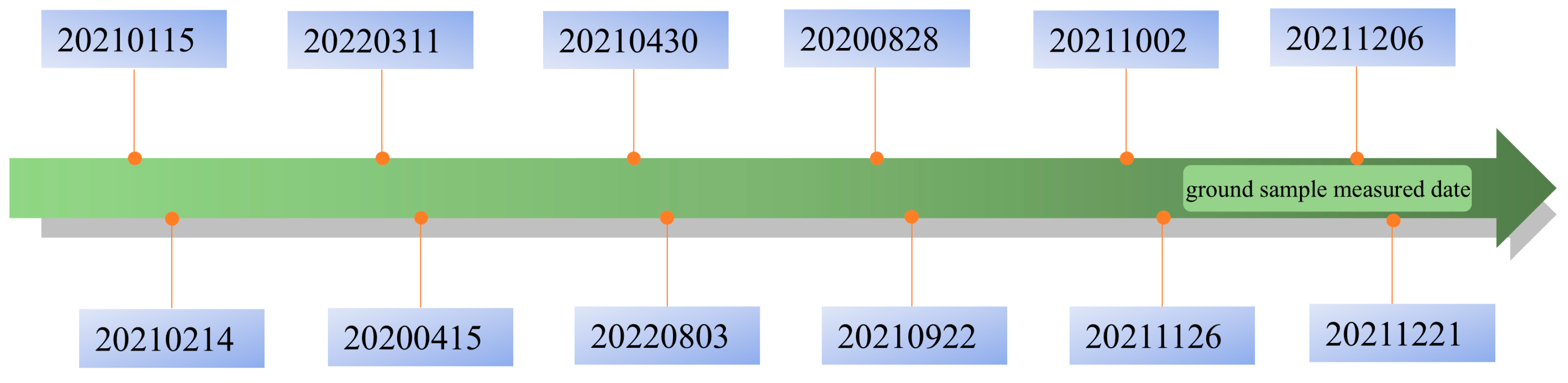
2.3. Remote Sensing Data and Pre-Processing
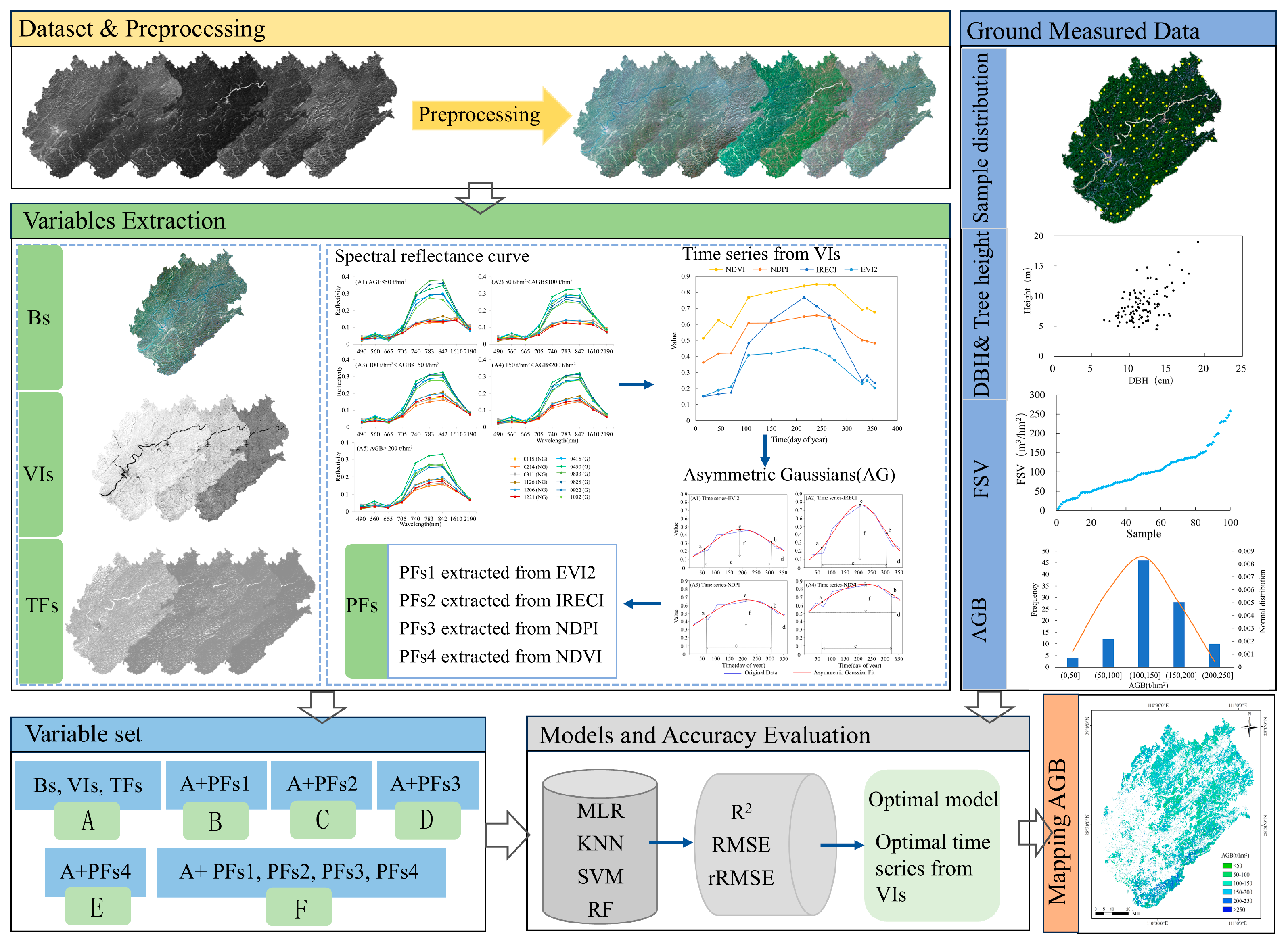
This study utilized Sentinel-2 time series data (Figure 2) from the Copernicus Data Space (https://dataspace.copernicus.eu/ accessed on 10 February 2025). To mitigate data gaps caused by cloud cover and precipitation, images from both 2020 and 2022 were composited. The preprocessing steps for Level-2A MSI data are as follows: (1) Orthorectification and radiometric correction to generate surface reflectance. (2) Relative radiometric normalization across acquisition dates. The September 22, 2021 image was selected as the reference for relative radiometric normalization. Pseudo-invariant features (PIFs) were identified and used to establish radiometric correction models between the reference and each subsequent acquisition. These models were then applied to normalize the complete time series of images. (3) The selection of nine key bands (blue, green, red, red-edge 1, red-edge 2, red-edge 3, near-infrared (NIR), short-wave infrared 1 (SWIR 1), and (SWIR 2); and (4) The resampling of 20 m resolution bands to 10 m. A 3 × 3 pixel window was subsequently applied to align the extracted remote sensing features with the target resolution.

3. Methods

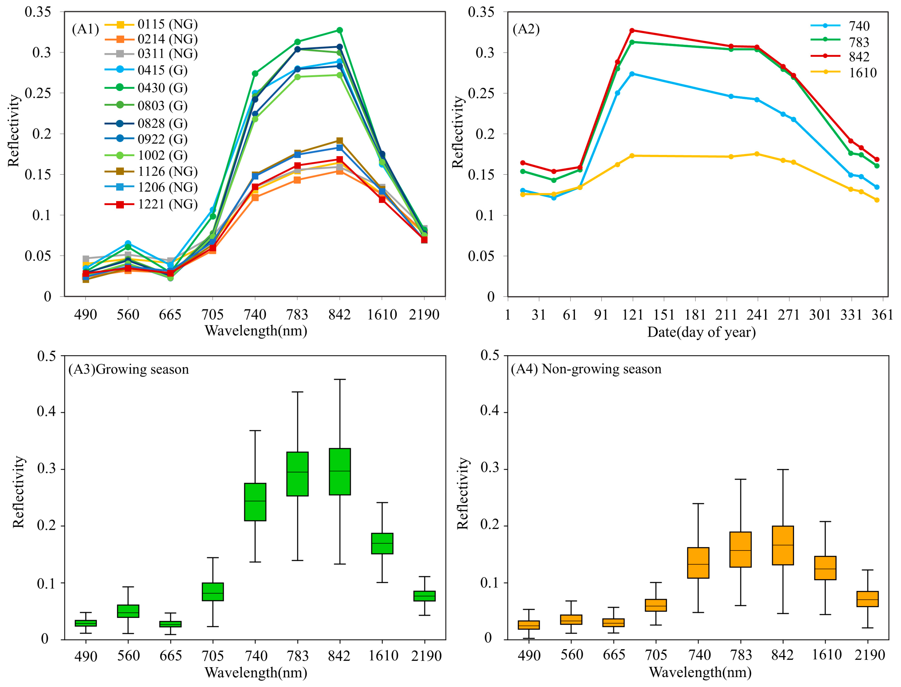
3.1. Spectral and Texture Features

The variables for evergreen broadleaf forest AGB mapping integrate three components: (1) spectral bands (Bs)—nine Sentinel-2 bands as foundational inputs; (2) vegetation indices (VI)—fourteen indices derived from spectral combinations, including the Normalized Difference Vegetation Index (NDVI), Soil-Adjusted Vegetation Index (SAVI), Atmospherically Resistant Vegetation Index (ARVI), Enhanced Vegetation Index 2 (EVI2), Red-Edge Chlorophyll Index (RECI), Green Normalized Difference Vegetation Index (GNDVI), Red-Green Vegetation Index (RGVI), Normalized Difference Phenology Index (NDPI), Optimized Soil-Adjusted Vegetation Index (OSAVI), Visible Atmospherically Resistant Index (VARI), Structure-Insensitive Pigment Index (SIPI), Green Chlorophyll Index (GCI), Normalized Difference Red-Edge Index (NDRE), and Inverted Red-Edge Chlorophyll Index (IRECI) [37,38]; and (3) texture features (TFs)—eight Gray-Level Co-occurrence Matrix (GLCM) texture features (mean, variance, homogeneity, contrast, dissimilarity, entropy, second moment, and correlation). These three components were extracted from the nine Bs using multi-scale moving windows (5 × 5, 7 × 7, 9 × 9, and 11 × 11 pixels).

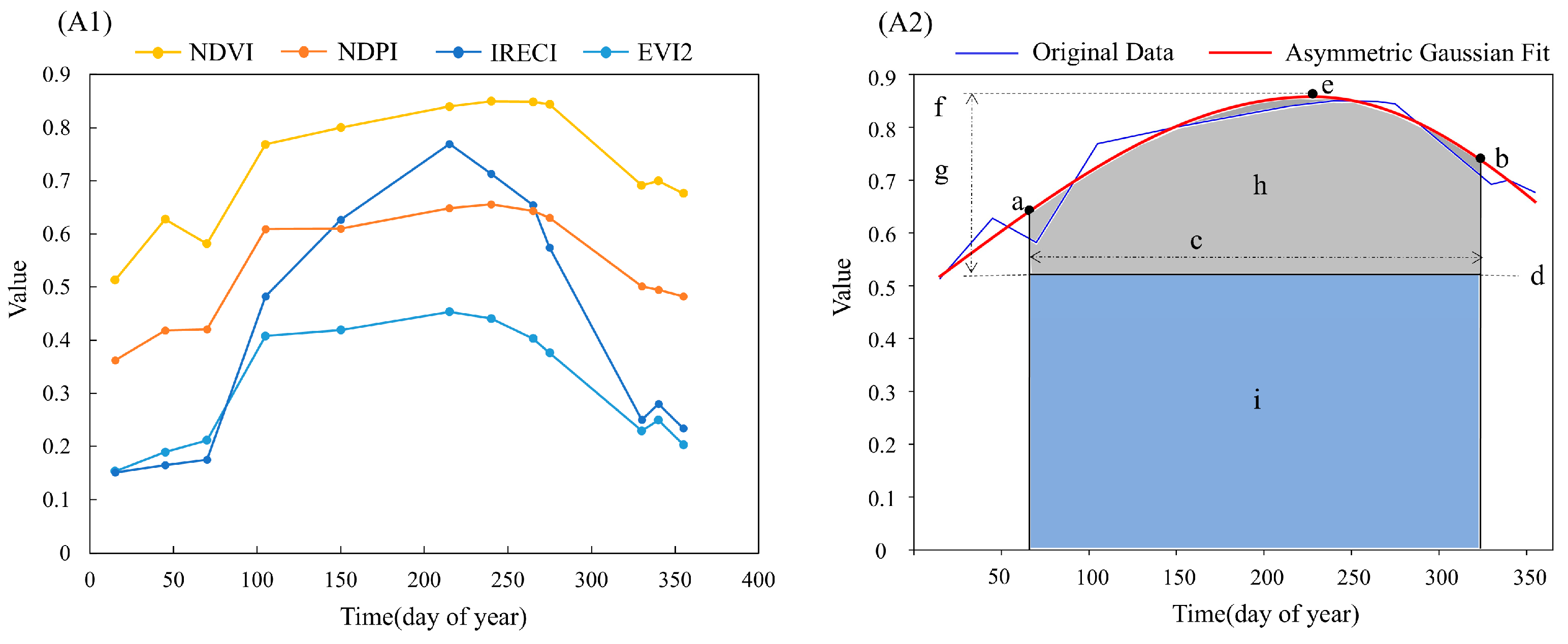
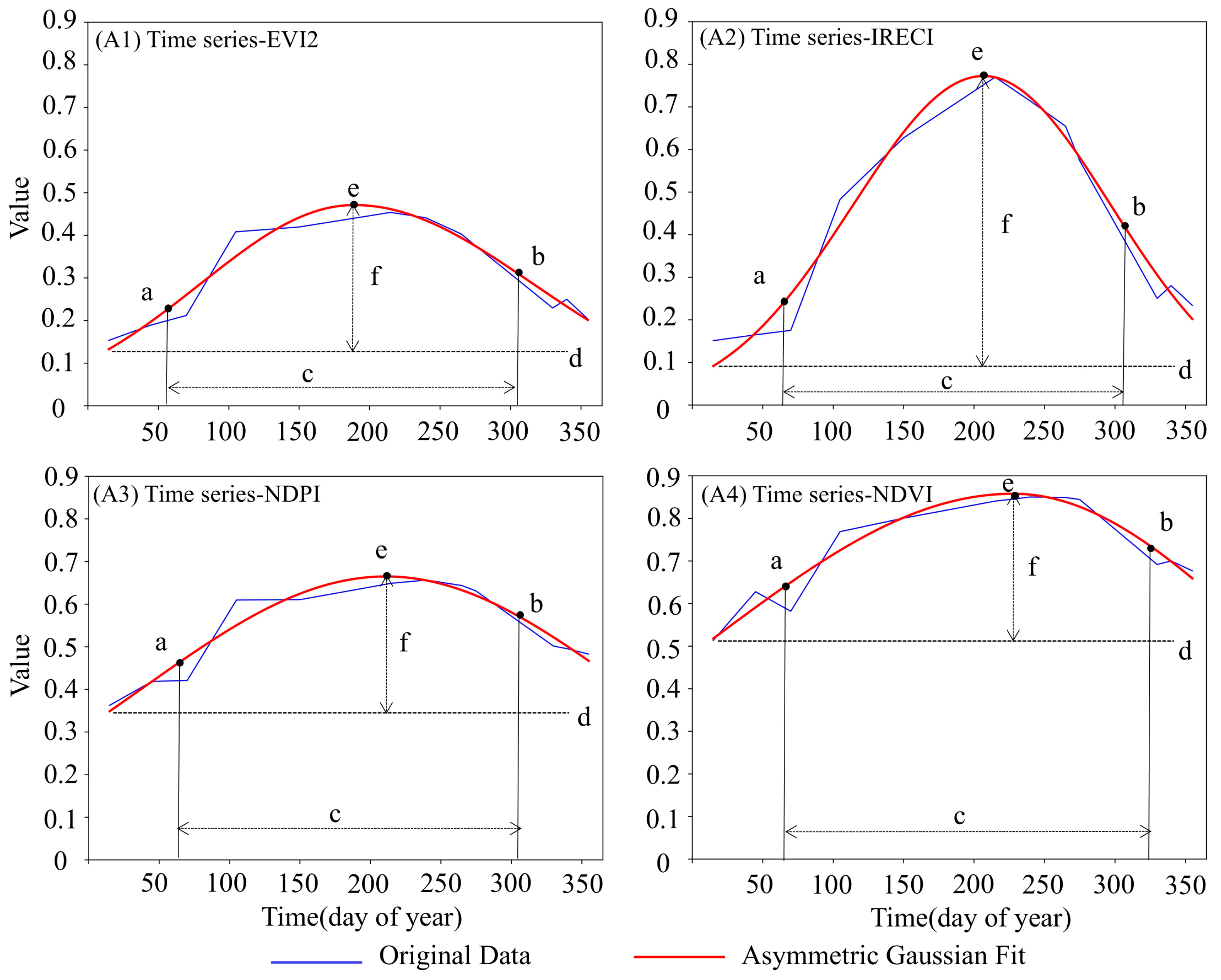
3.2. Phenological Features

Normally, phenological information can be observed via time series data. In this study, based on the sensitivity bands of the observation of phenology information in subtropical evergreen broadleaf forests, four VI, including EVI2, IRECI, NDPI, and NDVI, were employed to obtain the time series data. Both EVI2 and NDVI are calculated based on the red and near-infrared (NIR) bands. IRECI is derived from operations involving the red and red edge 1–3 bands. NDPI is obtained by utilizing data from the red, NIR, and SWIR-1 bands. Four time series VI (Figure 3A1), including EVI2, IRECI, NDPI, and NDVI, were employed to extract the PFs. These four-time series underwent a linear interpolation process to achieve a uniform distribution of time intervals.
Furthermore, the method for PFs extraction involves initially fitting the time series data, followed by determining the start of season (SOS) and end of season (EOS) using the dynamic threshold method [39]. In this study, all four series (Figure 3A1) depict the progression of the vegetation growth period in a manner resembling a Gaussian function. However, due to inherent growth characteristics, this is not necessary for the peak growing season to coincide with the midpoint of this period. As observed from Figure 3A1, these four curves representing vegetation index series exhibit an asymmetric distribution. Previous studies have illustrated that the Asymmetric Gaussian (AG) model developed by Jönsson and Eklundh, could be used for reconstructing time series data in broadleaf forests [40]. To accurately capture such asymmetrical features in this study, the AG model was employed to fit the curves.
f ( t ; c 1 , c 2 , x 1 , , x 5 ) = c 1 + c 2 g ( t ; x 1 , , x 5 )
where c 1 , c 2 are linear parameters and x 1 , , x 5 are non-linear parameters. c 1 , c 2 determine the base level and the amplitude. x 1 , , x 5 determine the shape of the base function that is the Gaussian function as followed:
g ( t ; x 1 , x 2 , , x 5 ) = exp t x 1 x 2 x 3     if     t > x 1 exp x 1 t x 4 x 5     if     t < x 1
where x1 determines the position of the maximum or minimum with respect to the independent time variable t, while x2 and x3 determine the width and flatness of the right function half. Similarly, x4 and x5 determine the width and flatness of the left half. To ensure smooth shapes of the model functions consistent with the observed data, restrictions are imposed on parameters x2 to x5. The application of the AG method necessitated a basic condition for time series analysis, as there are five free parameters in the AG model, implying that at least five valid observations are required [41].
The previous findings have demonstrated the high suitability of TIMESAT for investigations conducted at the local to regional scales [42]. Therefore, in this study, the TIMESAT 3.3 software was employed to extract PFs from a time series index (Figure 3A2). The extracted PFs primarily include the start of season timing (SOS), end of season timing (EOS), duration of the growing season (LOS), baseline value (BV), mid-season timing (MOS), maximum value attained by the fitted function during the growing season (MAXMUN), seasonal amplitude (AP), rate of increase at the onset of the growing season (LD), rate of decrease at the conclusion of the growing season (RD), large seasonal integral (LT), small seasonal integral (ST), SOS value, and EOS value.

3.3. Variables Sets

To evaluate the contribution of PFs in evergreen broadleaf forest AGB mapping, we designed a controlled experiment with six variable datasets (Table 2), structured sequentially as follows: Variable set A (baseline) combining 311 variables from Bs, VI, and TFs extracted from the 21 December 2021 image; Variable sets B–E incorporating PFs derived separately from time-series EVI2, IRECI, NDPI, and NDVI into set A, each generating 324 variables; and Variable set F (full combination) integrating all PFs from the four VI’ time-series data with set A to yield 363 total variables.
Additionally, a robust variable selection method was crucial for accurately estimating forest AGB. In this study, the variables were first evaluated using Euclidean distance correlation(DC) coefficients and ranked in descending order of their DC values. Based on this ranking, a forward feature selection method was then applied to sequentially identify features that provided the greatest improvement in model performance [43]. This approach followed the principle of iteratively selecting the most contributive features until no significant performance enhancement was observed. To evaluate the contribution of each feature in the feature set selected by models to the estimation of AGB, we used the random forest feature importance evaluation method in the Sklearn package of Python 3.10.

3.4. Models and Accuracy Evaluation in Mapping Forest AGB

The regression models for mapping forest AGB are commonly based on machine learning methods. In this study, four machine learning models were employed, including multiple linear regression (MLR), K-nearest neighbor (KNN), support vector machine (SVM), and random forest (RF). All models were implemented in Python 3.10 using the scikit-learn, Pandas, and NumPy libraries. The parameter settings for the models were as follows: MLR with L2 regularization (α = 0.01); KNN with the number of neighbors k restricted to integers between 1 and 50 (k ∈ ℤ ∩ [1, 50]); SVM with an RBF kernel, where the penalty parameter C and kernel coefficient γ were tuned via grid search across the ranges [0.1, 10] and [0.01, 1], respectively; and RF with a maximum tree depth constrained to [1, 15], 50 trees (n_estimators = 50), and depth optimization guided by out-of-bag (OOB) error. Additionally, the performances of these regression models were evaluated using Leave-One-Out Cross-Validation (LOOCV) through metrics such as the root mean square error (RMSE), relative root mean square error (rRMSE), and coefficient of determination (R2) [44]. The research framework is illustrated in Figure 4.

4. Results

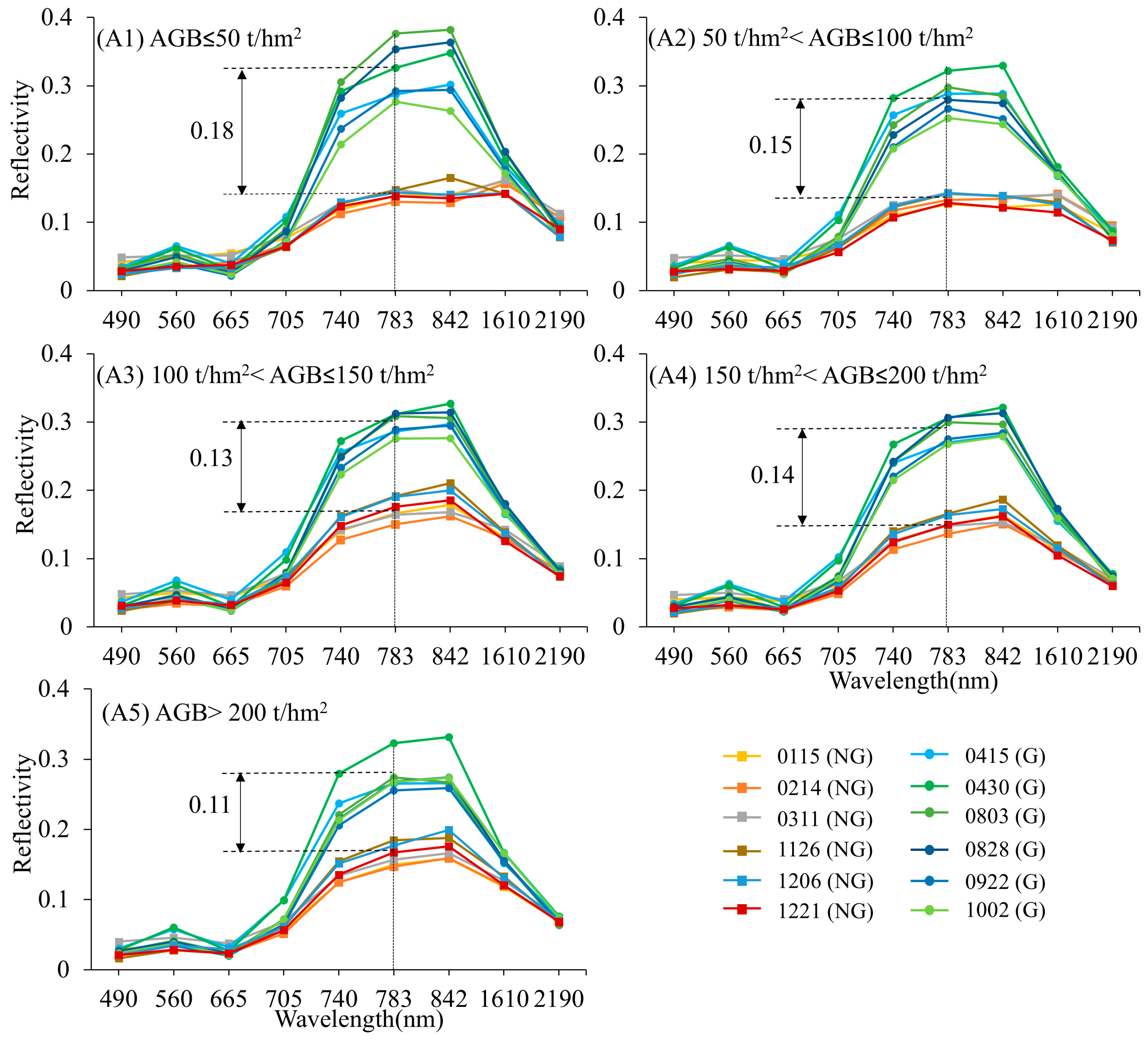
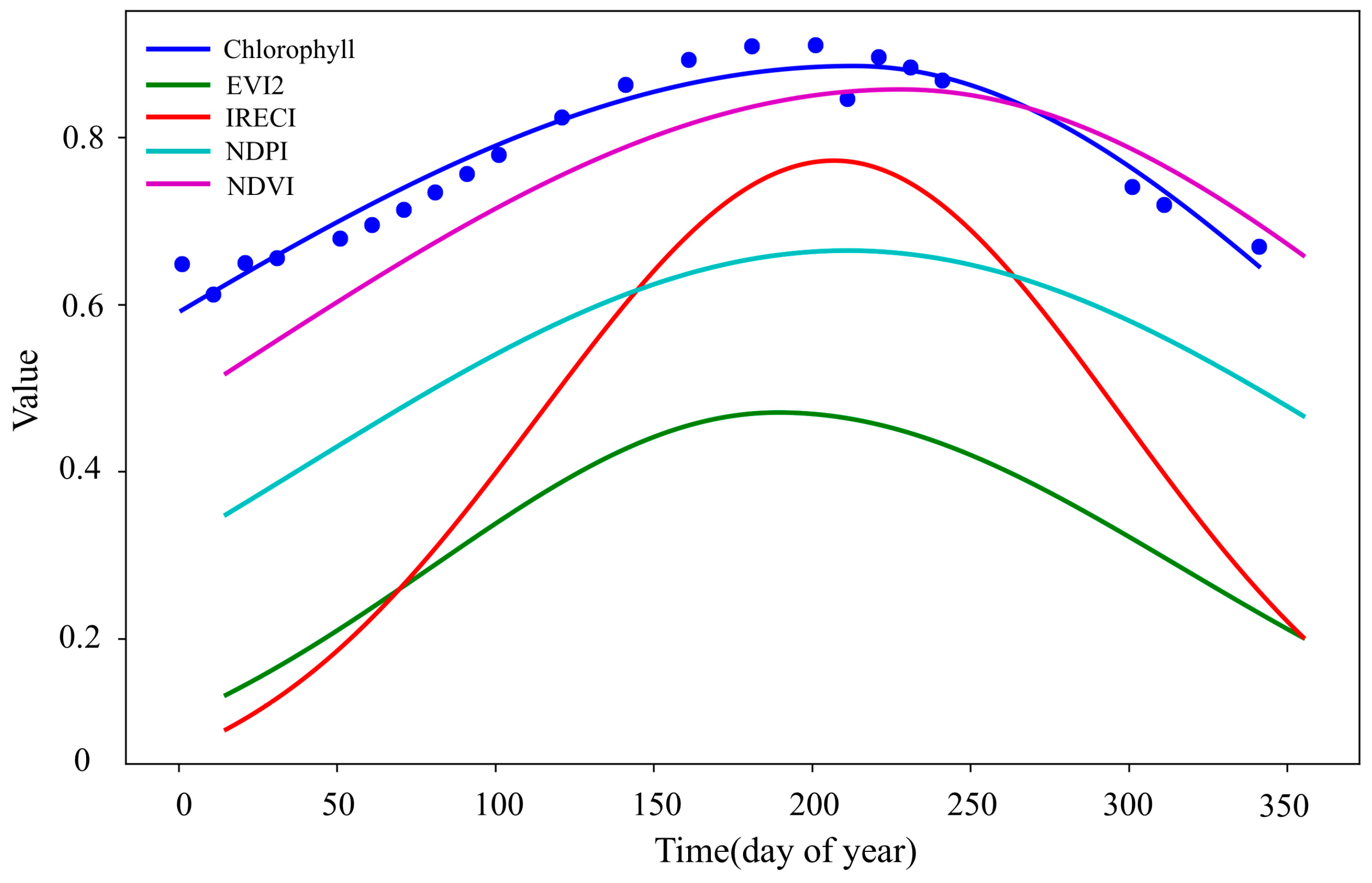
4.1. The Results of Spectral Response in Subtropical Evergreen Broadleaf Forests

A spectral analysis of nine bands showed significant variations between these seasons (Figure 5A1), with marked differences in the 740–1610 nm range. Four spectral sensitivity bands’ temporal profiles further validated these phenological contrasts (Figure 5A2). Quantitative evidence from mean reflectance boxplots (Figure 5A3,A4) consistently demonstrated seasonal spectral divergence. These findings confirm that subtropical evergreen broadleaf forests exhibit detectable phenological signals through spectral variations between the growing and non-growing seasons within 740–1610 nm.
To further investigate spectral reflectance-AGB relationships in subtropical evergreen broadleaf forests, all field survey plots were stratified into five 50 t/hm2 intervals (Table 1). Figure 6 displays the averaged spectral reflectance across all images for each AGB stratum. All five AGB strata showed noticeable reflectance differences within the 740–1610 nm spectral range. Additionally, the gaps between spectral reflectance during growing and non-growing seasons vary with forest AGB levels, showing significantly larger gaps in low AGB samples than in high AGB samples. In Figure 6, the maximum difference between the average reflectance in the growing season and the non-growing season is 0.18 (for AGB: 0–50 t/hm²), while the minimum is 0.11 (for AGB > 200 t/hm²). The reflectance differences for the two AGB ranges of 100–150 t/hm² and 150–200 t/hm² exhibit an inverse trend. However, the overall trend shows that the differences decrease with an increasing AGB.

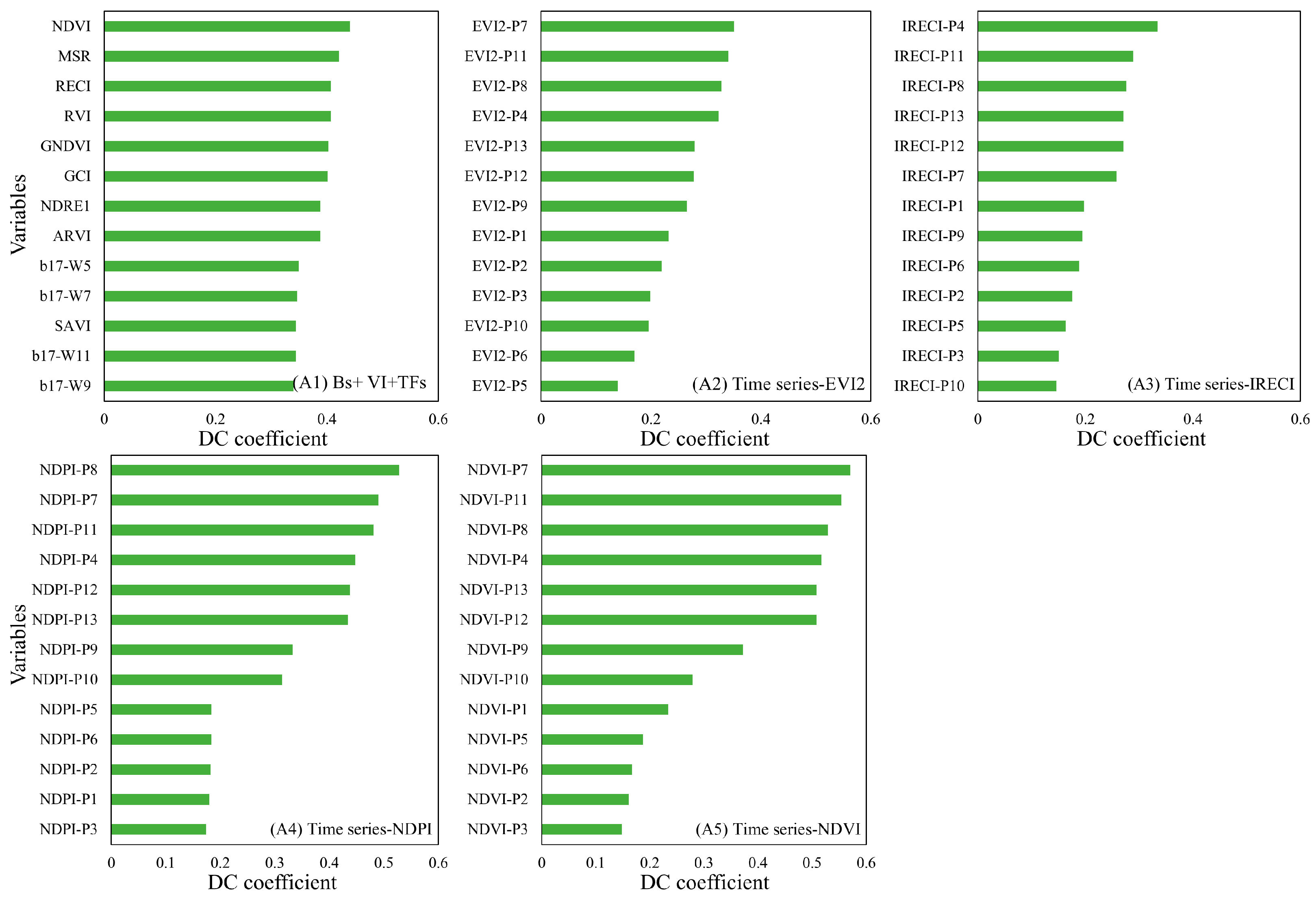
4.2. The Sensitivity Between the Forest AGB and the Extracted Phenological Features

Amongst these four fitting curves (Figure 7), the maximum value for the fitted function during the season (MAXMUN) of the time series NDVI fitting curve is the highest, while the MAXMUN of the time series EVI2 fitting curve is the lowest (Table 3). The time series IRECI exhibits both the highest amplitude (AP) and lowest base value (BV) among all the curves. There were minimal differences in the SOS, EOS, and LOS extracted from these four time-series data. The main differences were observed in the AP, BV and MAXMUN.
In constructing the regression models, the sensitivity between the features and AGB served as a crucial indicator for predicting AGB mapping contribution. In this study, the sensitivity between the forest AGB and various types of features, including spectral reflectance, VI, TFs, and PFs, was evaluated using distance correlation (DC) coefficients (Figure 8). The DC coefficient was separately calculated for each variable set with respect to the AGB and sorted in descending order. Specifically, 13 PFs were extracted from each time series vegetation index; furthermore, based on their DC coefficients, the Bs + VI + TFs variable set also selected the top 13 features.
The results demonstrate that the maximum value of the DC coefficient for the PFs (0.57) was significantly higher than that for the Bs + VI + TFs variable set (0.44). There were 10 PFs whose DC coefficients (ranging from 0.45 to 0.57) exceeded the maximum value of the Bs + VI + TFs variable set, indicating a greater sensitivity of the PFs to AGB estimation. Differences in feature sensitivity were observed among the PFs derived from the four VI. The time series-EVI2 and time series-IRECI exhibited maximum values of DC coefficients ranging from 0.3 to 0.4, while the time series NDVI and time series NDPI showed maximum values distributed within the range of 0.5 to 0.6. These findings demonstrate that PFs exhibit higher sensitivity to AGB compared to the Bs + VI + TFs variable set.

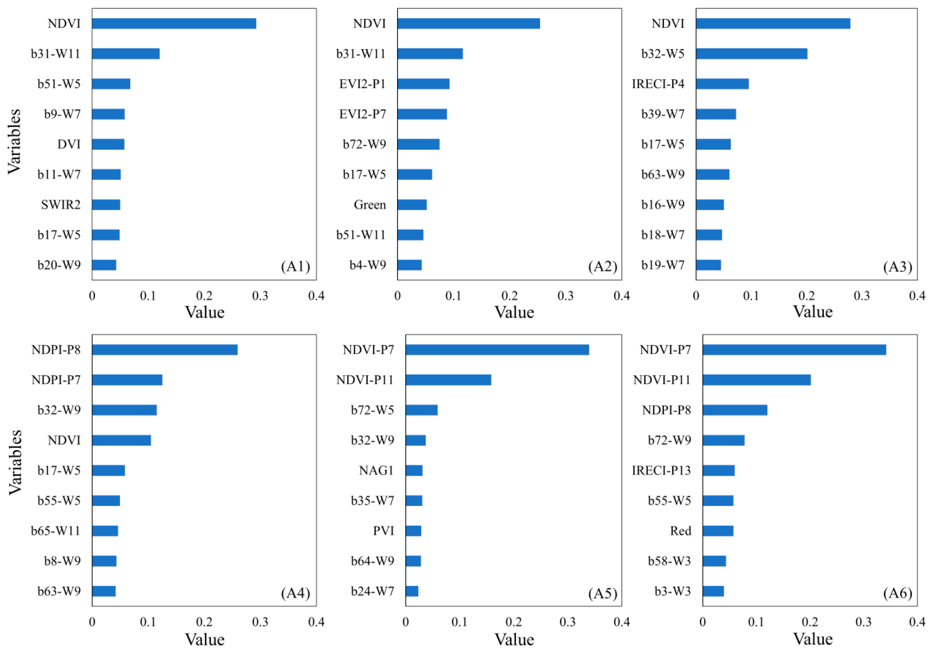
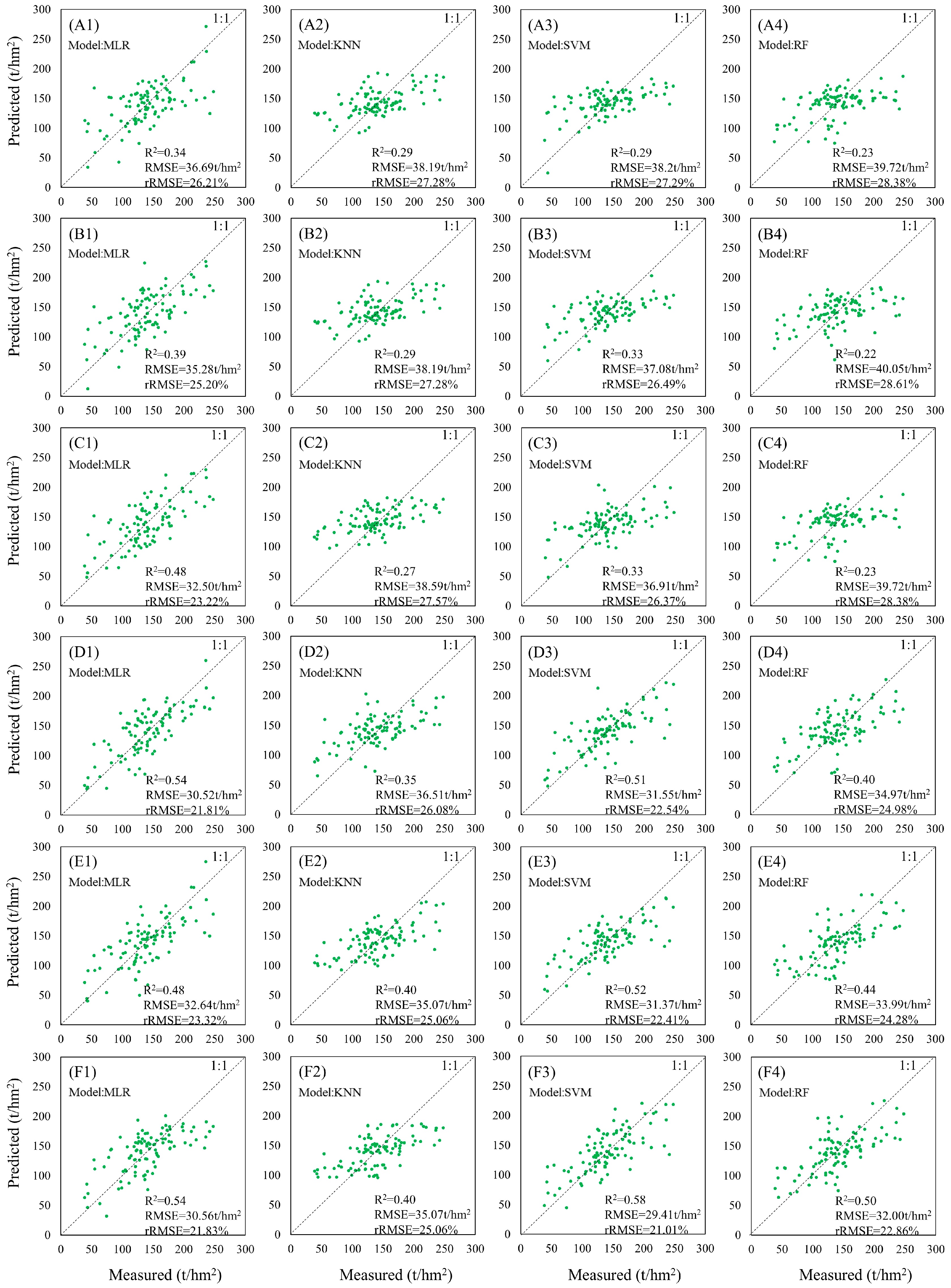
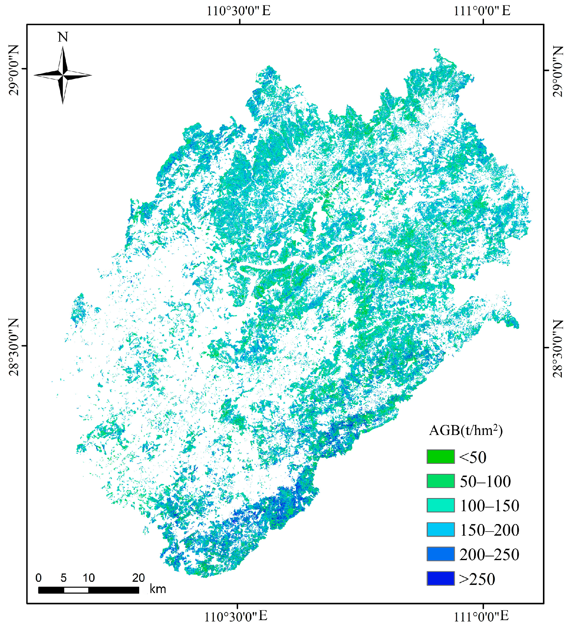
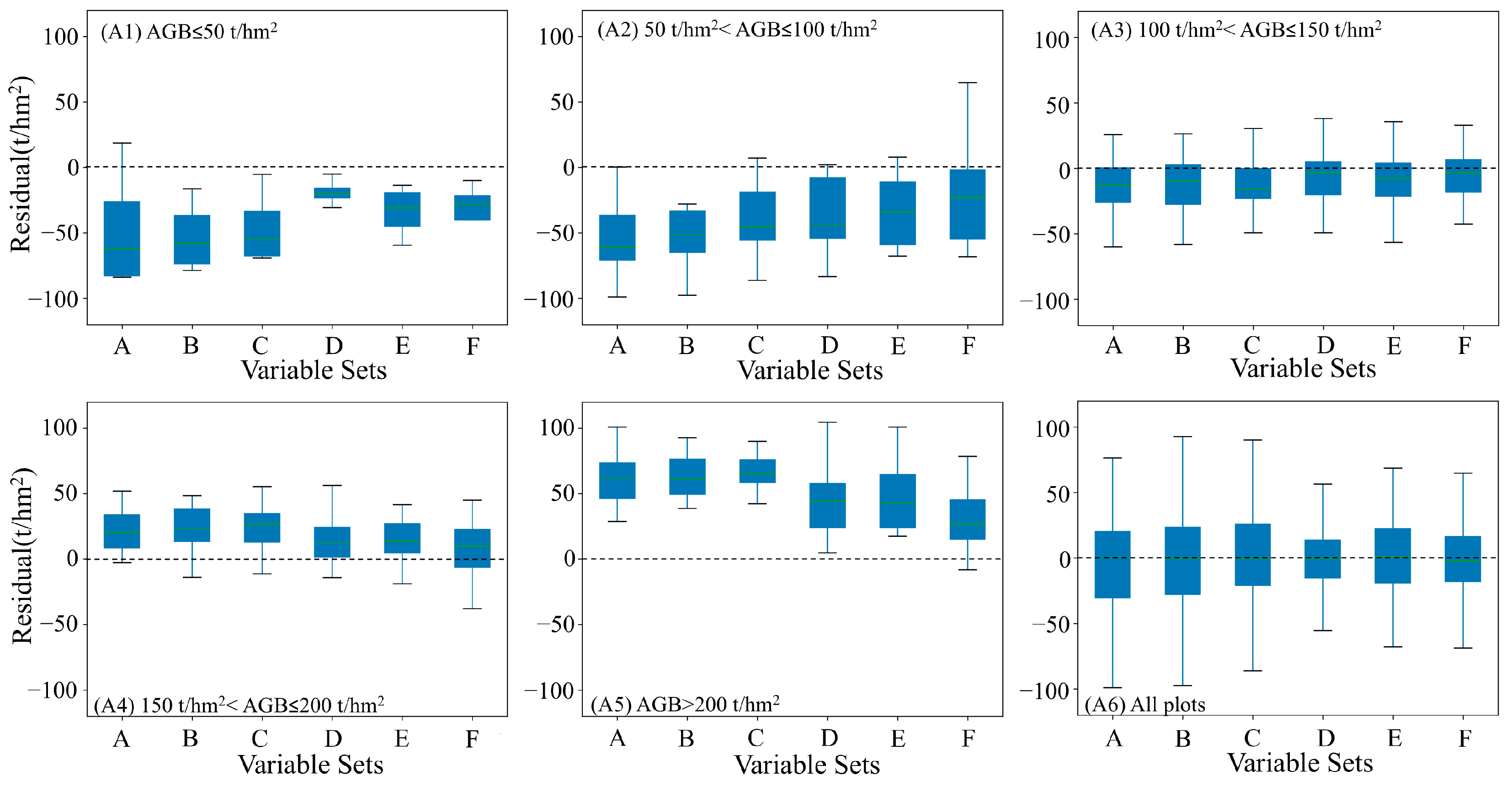
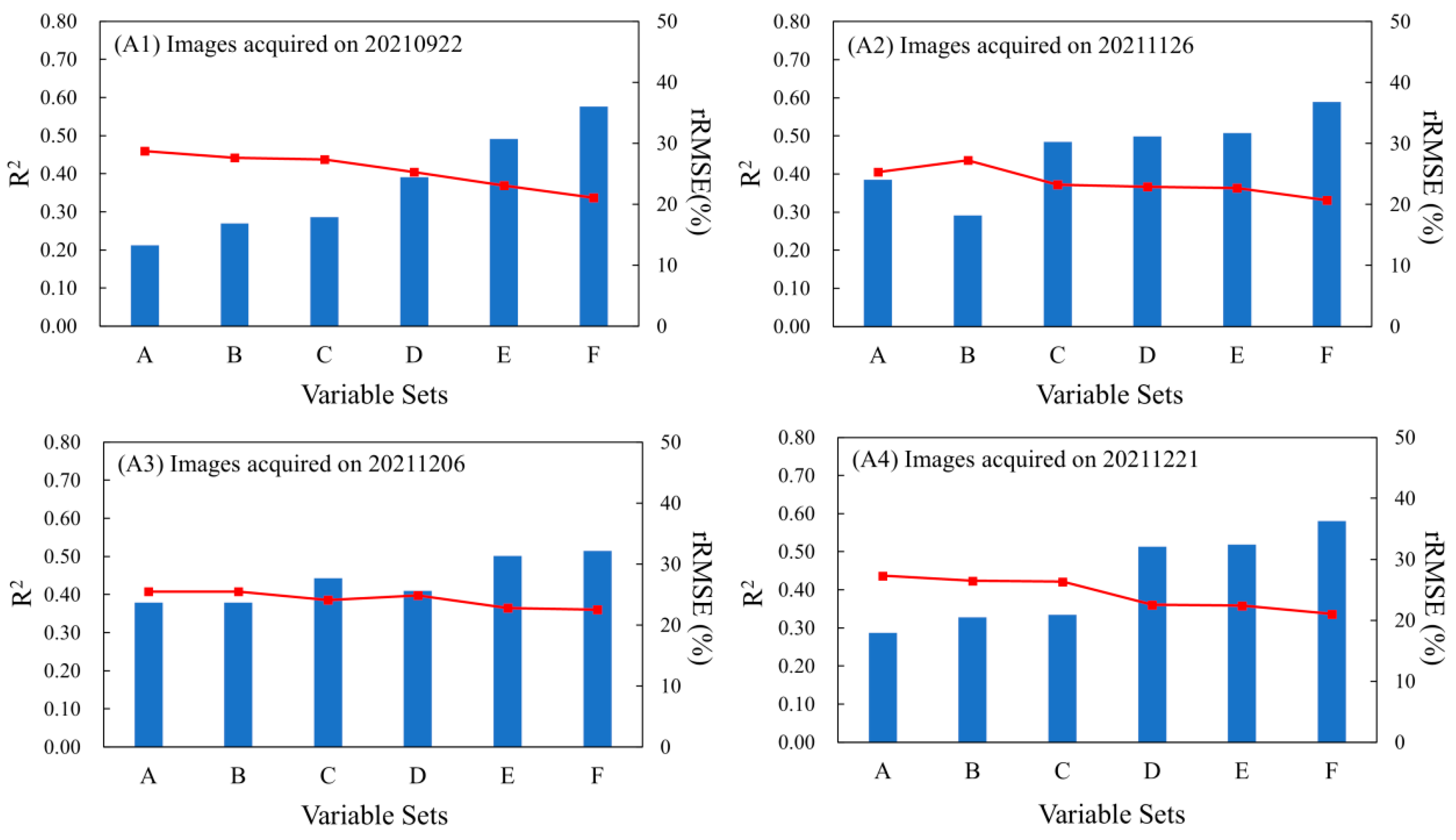
4.3. The Results of Mapping AGB

To evaluate the contribution of PFs within each optimal subset, we calculated feature importance using random forest for the selected feature subsets. The assessment results were then ranked in descending order, with the top nine features from each variable set being selected (Figure 9). The results illustrate that NDVI (0.29) is the most important feature in variable set A (Bs + VI + TFs). Amongst the variables encompassing PFs (A2–A6), all PFs exhibited significant contributions within each optimal subset. Notably, the top three most important features were all related to phenology. Regarding feature importance within the time series of NDVI and NDPI, PFs ranked first, with NDPI-P8 (LD, 0.26) and NDVI-P7 (AP, 0.34) being particularly influential. Furthermore, among combinations of PFs for each vegetation index in combination set A6, the top three most important features were NDVI-P7 (AP, 0.34), NDVI-P11 (ST, 0.20), and NDPI-P8 (LD, 0.12). It can be inferred that PFs play a significant role in optimizing feature subsets and have great potential for accurately mapping AGB in evergreen broadleaf forests.
After obtaining the optimal subset, four regression models, including MLR, SVM, KNN, and RF models, were constructed to accurately map the AGB in evergreen broadleaf forests. Control experiments were conducted using six variable sets (Table 2) to demonstrate the influence of PFs extracted from various time series VI on AGB estimation (Table 4). The results demonstrated that variable set A yielded rRMSE values ranging from 26.21% to 28.38% and R2 values ranging from 0.23 to 0.34. After combing variable set A with PFs extracted from various time series indices, the accuracy of mapping forest AGB improved, and the result of the greatest accuracy improvement was observed in variable set D (R2: ranged from 0.35 to 0.54; rRMSE: ranged from 21.81% to 26.08%) and variable set E (R2: ranged from 0.40 to 0.52; rRMSE: ranged from 22.41% to 24.28%). It is inferred that PFs have great potential in enhancing the accuracy of mapping AGB in subtropical evergreen broadleaf forests. Furthermore, the contribution of PFs derived from the time series NDVI and NDPI surpasses that of features extracted from the time series EVI2 and IRECI.
Furthermore, the integration of diverse PFs derived from all four VI significantly enhanced the accuracy in mapping AGB, with variable set F yielding rRMSE values ranging from 21.01% to 25.06% and R2 values ranging from 0.40 to 0.58. These results suggest that incorporating PFs extracted from various time series data also contributed to improving the precision of AGB mapping. In this study, the KNN model exhibited a relatively lower estimation accuracy compared to the other models. Nevertheless, as the quality of feature sets improved, the influence of model selection on estimation accuracy gradually diminished for AGB mapping purposes. This implies that prioritizing enhanced correlation and reliability within feature sets is more critical than selecting specific regression models for improving AGB accuracy.
To evaluate model performance, scatter plots were generated to demonstrate the relationships between predicted and ground-measured AGB for all samples (Figure 10). The results revealed that variable sets D, E, and F demonstrated improvements in reducing the underestimation of high values and overestimation of low values compared to variable set A. Notably, variable set F, which incorporated various vegetation index PFs, greatly enhanced the accuracy of AGB estimation for evergreen broadleaf forests.
Based on the optimal results from the regression models and variable sets, the forest AGB distribution map across the study area was generated using the SVM model with variable set F (Figure 11). It can be observed that most of the evergreen broadleaf forests in the study area had an AGB ranging from 50 to 250 t/hm2. Approximately 55% of evergreen broadleaf forests exhibit an AGB between 100 and 200 t/hm2. High levels of AGB are concentrated in the mountainous areas located in the southeast and northwest regions, consistent with the field survey sample plots.

5. Discussion

5.1. Interpretation the Phenological Features in Broadleaf Evergreen Forests

In northern deciduous forests, the observable changes in leaf color and leaf litter facilitate phenological monitoring [45]. However, accurately capturing the phenology of subtropical evergreen broadleaf forests becomes challenging due to the absence of significant changes in leaf color [46]. To address this issue, time-series Sentinel-2 remote sensing images were employed to construct spectral reflection curves for evergreen broadleaf forests across different months (Figure 5). The temporal patterns of these reflection spectra exhibited periodic fluctuations in foliage, indicating transitions from leaf emergence to maturity within these vegetation types. Moreover, the nine bands of Sentinel-2 not only observe visible leaf color temporal changes but also capture other variations during phenological periods. The results demonstrated the potential for monitoring phenological phenomena in subtropical broadleaf evergreen forests through the analysis of vegetation surface reflectance, thereby providing a theoretical basis for selecting appropriate VI to extract relevant PFs. Additionally, our results also revealed a distinct seasonal stratification in reflectance between wavelengths ranging from 740 nm to 1610 nm within evergreen broadleaf forest ecosystems. Based on this pattern of spectral variation, four VI (EVI2, IRECI, NDPI, and NDVI) were selected to construct time series VI that would effectively capture key PFs.
Previous studies have demonstrated that solar radiation and spectral composition exert significant influences on forest phenology. Trees at higher latitudes exhibit greater sensitivity to changes in their red/far-red (R:FR) ratio [47]. In temperate deciduous forests, there is a significant correlation between the greenness and redness indices over the germination and leaf emergence time of individual trees in spring [48]. These indices are greatly influenced by leaf discoloration and senescence. On the contrary, the evergreen broadleaf forest studied here is located in a low latitude area, where it has been found that phenological changes are sensitive to the red edge and near-infrared bands through spectral reflectance analysis [49,50]. Vegetation indices (VIs) serve as convenient proxies for canopy structure and leaf pigment content. Both NDVI and EVI2 demonstrate good capabilities for monitoring phenology [51]. Additionally, NDVI shows a high correlation with autumn phenology and is widely used for extracting phenological information [52,53]. In this study, the disparities observed among the four time series datasets primarily manifest in terms of AP, BV, and MOS, resulting in varying degrees of sensitivity towards AGB. The PFs derived from NDVI and NDPI exhibit heightened sensitivity towards AGB, while those obtained from EVI2 and IRECI demonstrate comparatively lower levels of sensitivity.
Furthermore, the MuSyQ LCC leaf chlorophyll products [54] were also utilized to further investigate the discrepancy between the time series data, enabling an evaluation of phenological changes in the vegetation canopy. Asymmetric Gaussian fitting was applied to four time series and subsequently compared with the fitting curve of MuSyQ LCC (Figure 12). The trends observed in the time series NDVI and NDPI are consistent with those of MuSyQ LCC, indicating that NDVI and NDPI provide a more direct reflection of phenological changes in evergreen broadleaf forests compared to EVI2 and IRECI.

5.2. Potential of Phenological Features on AGB Mapping

Mapping AGB with remote sensing images in evergreen broadleaf forests has challenges [55]. This study introduced PFs to enhance the precision of AGB estimation. The results demonstrated that incorporating PFs significantly improves the accuracy of AGB estimation. To further assess the reliability and validity of the results, a box plot (Figure 13) was constructed to visualize the residual errors between the predicted and ground measured AGB. The results demonstrated that for AGB < 100 t/hm2, the underestimated samples could be clearly observed for six variable sets, with the dataset lacking PFs exhibiting a more pronounced underestimation. Conversely, for AGB > 150 t/hm2, all datasets exhibited spectral signal saturation; however, the variable sets with PFs significantly mitigated this effect. These findings show complete agreement with the patterns demonstrated in the scatter plots (Figure 10). It is inferred that the potential of PFs is not only in alleviating saturation issues in remote sensing signals but also in improving low-value overestimations. Furthermore, comparing the residuals among the six variable sets in Figure 13 reveals that utilizing NDVI and NDPI time series data for extracting PFs greatly enhances the accuracy of AGB estimation compared to EVI2 and IRECI.
Furthermore, the universality of PFs was further verified through the collection of remote sensing data in adjacent months. In this study, the SVM model was employed to estimate AGB for images acquired on 22 September, 26 November, 6 December, and 12 December (Figure 14) The overall consistency of the model’s estimation results across these four images demonstrates the effectiveness of utilizing PFs from vegetation index time series in estimating AGB. Previous studies have shown that seasonal NDVI time series can yield more accurate AGB estimates compared to single NDVI measurements [56]. Constructing composite images and extracting PFs from time series data have also been proven to enhance forest stock estimation accuracy [57]. Moreover, there are studies employing long-term optical time models to improve AGB estimation accuracy and achieve AGB dynamic monitoring specifically for temperate tree species [58]. The results inferred that phenology features can be considered a key factor for alleviating spectral signal saturation problems while effectively improving the accuracy of AGB estimation.

6. Conclusions

To enhance the accuracy of AGB mapping and mitigate the impact of saturation phenomena in evergreen broadleaf forests, a time series dataset was constructed using Sentinel-2 optical remote sensing images to investigate variations in spectral reflectance during both the non-growing and growing seasons. Subsequently, four time series VI (EVI2, IRECI, NDVI, and NDPI) were utilized to extract phenology features for the development of regression models aimed at addressing challenges associated with spectral saturation when accurately estimating AGB. The results demonstrated that phenological information of subtropical evergreen broadleaf forests can be observed through variations between the growing and non-growing seasons within a wavelength range spanning from 740 nm to 1610 nm. Moreover, the maximum value of the DC coefficient for PFs (0.57) was significantly higher than that for the Bs + VI + TFs variable set (0.44). Compared with EVI2 (R2 = 0.33) and IRECI (R2 = 0.33), it is indicated that the PFs extracted from the NDVI (R2 = 0.52) and NDPI (R2 = 0.51) timing data significantly improved the accuracy of estimating AGB in evergreen broadleaf forests. The highest accuracy for AGB estimation was achieved by combining all four vegetation indices’ PFs. In future studies, we will conduct an in-depth analysis of surface reflectance variations across different spectral bands to identify more sensitive phenological indicators from reflectance time-series patterns.

Author Contributions

Conceptualization, P.Y., J.L. and Z.L.; methodology, P.Y.; software, P.Y. and T.Z.; validation, P.Y.; formal analysis, P.Y.; investigation, Z.Y. and T.Z.; resources, P.Y., Z.Y. and T.Z.; data curation, P.Y.; writing—original draft preparation, P.Y.; writing—review and editing, P.Y. and J.L.; visualization, P.Y.; supervision, H.L.; project administration, H.L.; funding acquisition, J.L. All authors have read and agreed to the published version of the manuscript.

Funding

This research was funded by National Natural Science Foundation of China (Project number: 32171784) and postgraduate scientific research Innovative project of Hunan province (Project number: CX20230778). We would also like to thank the anonymous reviewers for their useful comments and constructive suggestions.

Data Availability Statement

The observed AGB data from the sample plots and spatial distribution data of forest resources presented in this study are available on request from the corresponding author. These data are not publicly accessible due to privacy and confidentiality concerns. The Sentinel-2 images are available from the Copernicus Data Space Ecosystem. (https://browser.dataspace.copernicus.eu, accessed on 31 December 2022).

Conflicts of Interest

The authors declare no conflicts of interest.

References

  1. Araujo, E.C.G.; Sanquetta, C.R.; Dalla Corte, A.P.; Pelissari, A.L.; Orso, G.A.; Silva, T.C. Global review and state-of-the-art of biomass and carbon stock in the Amazon. J. Environ. Manag. 2023, 331, 117251. [Google Scholar] [CrossRef] [PubMed]
  2. Lu, D.S.; Chen, Q.; Wang, G.X.; Liu, L.J.; Li, G.Y.; Moran, E. A survey of remote sensing-based aboveground biomass estimation methods in forest ecosystems. Int. J. Digit. Earth 2016, 9, 63–105. [Google Scholar] [CrossRef]
  3. Abbas, S.; Wong, M.S.; Wu, J.; Shahzad, N.; Irteza, S.M. Approaches of Satellite Remote Sensing for the Assessment of Above-Ground Biomass across Tropical Forests: Pan-tropical to National Scales. Remote Sens. 2020, 12, 3351. [Google Scholar] [CrossRef]
  4. Latifi, H.; Fassnacht, F.E.; Hartig, F.; Berger, C.; Hernandez, J.; Corvalan, P.; Koch, B. Stratified aboveground forest biomass estimation by remote sensing data. Int. J. Appl. Earth Obs. Geoinf. 2015, 38, 229–241. [Google Scholar] [CrossRef]
  5. Ploton, P.; Barbier, N.; Couteron, P.; Antin, C.M.; Ayyappan, N.; Balachandran, N.; Barathan, N.; Bastin, J.F.; Chuyong, G.; Dauby, G.; et al. Toward a general tropical forest biomass prediction model from very high resolution optical satellite images. Remote Sens. Environ. 2017, 200, 140–153. [Google Scholar] [CrossRef]
  6. Ahmad, A.; Gilani, H.; Ahmad, S.R. Forest Aboveground Biomass Estimation and Mapping through High-Resolution Optical Satellite Imagery-A Literature Review. Forests 2021, 12, 914. [Google Scholar] [CrossRef]
  7. Dube, T.; Mutanga, O. Evaluating the utility of the medium-spatial resolution Landsat 8 multispectral sensor in quantifying aboveground biomass in uMgeni catchment, South Africa. Isprs J. Photogramm. Remote Sens. 2015, 101, 36–46. [Google Scholar] [CrossRef]
  8. McRoberts, R.E.; Naesset, E.; Gobakken, T. Optimizing the k-Nearest Neighbors technique for estimating forest aboveground biomass using airborne laser scanning data. Remote Sens. Environ. 2015, 163, 13–22. [Google Scholar] [CrossRef]
  9. Wang, J.; Xiao, X.; Bajgain, R.; Starks, P.; Steiner, J.; Doughty, R.B.; Chang, Q. Estimating leaf area index and aboveground biomass of grazing pastures using Sentinel-1, Sentinel-2 and Landsat images. ISPRS J. Photogramm. Remote Sens. 2019, 154, 189–201. [Google Scholar] [CrossRef]
  10. Silveira, E.M.O.; Silva, S.H.G.; Acerbi-Junior, F.W.; Carvalho, M.C.; Carvalho, L.M.T.; Scolforo, J.R.S.; Wulder, M.A. Object-based random forest modelling of aboveground forest biomass outperforms a pixel-based approach in a heterogeneous and mountain tropical environment. Int. J. Appl. Earth Obs. Geoinf. 2019, 78, 175–188. [Google Scholar] [CrossRef]
  11. David, R.M.; Rosser, N.J.; Donoghue, D.N.M. Improving above ground biomass estimates of Southern Africa dryland forests by combining Sentinel-1 SAR and Sentinel-2 multispectral imagery. Remote Sens. Environ. 2022, 282, 19. [Google Scholar] [CrossRef]
  12. Liu, Y.; Gong, W.; Xing, Y.; Hu, X.; Gong, J. Estimation of the forest stand mean height and aboveground biomass in Northeast China using SAR Sentinel-1B, multispectral Sentinel-2A, and DEM imagery. ISPRS J. Photogramm. Remote Sens. 2019, 151, 277–289. [Google Scholar] [CrossRef]
  13. Lin, H.; Zhao, W.G.; Long, J.P.; Liu, Z.H.; Yang, P.S.; Zhang, T.C.; Ye, Z.L.; Wang, Q.Y.; Matinfar, H.R. Mapping Forest Growing Stem Volume Using Novel Feature Evaluation Criteria Based on Spectral Saturation in Planted Chinese Fir Forest. Remote Sens. 2023, 15, 402. [Google Scholar] [CrossRef]
  14. Cao, L.; Coops, N.C.; Innes, J.L.; Sheppard, S.R.J.; Fu, L.; Ruan, H.; She, G. Estimation of forest biomass dynamics in subtropical forests using multi-temporal airborne LiDAR data. Remote Sens. Environ. 2016, 178, 158–171. [Google Scholar] [CrossRef]
  15. Liao, Z.; Liu, X.; van Dijk, A.; Yue, C.; He, B. Continuous woody vegetation biomass estimation based on temporal modeling of Landsat data. Int. J. Appl. Earth Obs. Geoinf. 2022, 110, 102811. [Google Scholar] [CrossRef]
  16. Fu, Y.C.; Li, R.H.; Zhu, Z.; Xue, Y.F.; Ding, H.; Wang, X.Y.; Na, J.M.; Xia, W.J. SCARF: A new algorithm for continuous prediction of biomass dynamics using machine learning and Landsat time series. Remote Sens. Environ. 2024, 314, 17. [Google Scholar] [CrossRef]
  17. Li, Q.Y.; Lin, H.; Long, J.P.; Liu, Z.H.; Ye, Z.L.; Zheng, H.N.; Yang, P.S. Mapping Forest Stock Volume Using Phenological Features Derived from Time-Serial Sentinel-2 Imagery in Planted Larch. Forests 2024, 15, 995. [Google Scholar] [CrossRef]
  18. Arevalo, P.; Baccini, A.; Woodcock, C.E.; Olofsson, P.; Walker, W.S. Continuous mapping of aboveground biomass using Landsat time series. Remote Sens. Environ. 2023, 288, 113483. [Google Scholar] [CrossRef]
  19. Nguyen, T.H.; Jones, S.; Soto-Berelov, M.; Haywood, A.; Hislop, S. Landsat Time-Series for Estimating Forest Aboveground Biomass and Its Dynamics across Space and Time: A Review. Remote Sens. 2020, 12, 98. [Google Scholar] [CrossRef]
  20. Caparros-Santiago, J.A.; Rodriguez-Galiano, V.; Dash, J. Land surface phenology as indicator of global terrestrial ecosystem dynamics: A systematic review. ISPRS J. Photogramm. Remote Sens. 2021, 171, 330–347. [Google Scholar] [CrossRef]
  21. Dronova, I.; Taddeo, S. Remote sensing of phenology: Towards the comprehensive indicators of plant community dynamics from species to regional scales. J. Ecol. 2022, 110, 1460–1484. [Google Scholar] [CrossRef]
  22. Thapa, S.; Garcia Millan, V.E.; Eklundh, L. Assessing Forest Phenology: A Multi-Scale Comparison of Near-Surface (UAV, Spectral Reflectance Sensor, PhenoCam) and Satellite (MODIS, Sentinel-2) Remote Sensing. Remote Sens. 2021, 13, 1597. [Google Scholar] [CrossRef]
  23. Decuyper, M.; Chavez, R.O.; Lohbeck, M.; Lastra, J.A.; Tsendbazar, N.; Hacklander, J.; Herold, M.; Vagen, T.-G. Continuous monitoring of forest change dynamics with satellite time series. Remote Sens. Environ. 2022, 269, 112829. [Google Scholar] [CrossRef]
  24. Li, L.W.; Li, N.; Zang, Z.; Lu, D.S.; Wang, G.X.; Wang, N. Examining phenological variation of on-year and off-year bamboo forests based on the vegetation and environment monitoring on a New Micro-Satellite (VENμS) time-series data. Int. J. Remote Sens. 2021, 42, 2203–2219. [Google Scholar] [CrossRef]
  25. Lara, B.; Gandini, M. Assessing the performance of smoothing functions to estimate land surface phenology on temperate grassland. Int. J. Remote Sens. 2016, 37, 1801–1813. [Google Scholar] [CrossRef]
  26. Tan, B.; Morisette, J.T.; Wolfe, R.E.; Gao, F.; Ederer, G.A.; Nightingale, J.; Pedelty, J.A. An Enhanced TIMESAT Algorithm for Estimating Vegetation Phenology Metrics From MODIS Data. IEEE J. Sel. Top. Appl. Earth Observ. Remote Sens. 2011, 4, 361–371. [Google Scholar] [CrossRef]
  27. Zeng, L.L.; Wardlow, B.D.; Xiang, D.X.; Hu, S.; Li, D.R. A review of vegetation phenological metrics extraction using time-series, multispectral satellite data. Remote Sens. Environ. 2020, 237, 111511. [Google Scholar] [CrossRef]
  28. Cao, R.; Chen, Y.; Shen, M.; Chen, J.; Zhou, J.; Wang, C.; Yang, W. A simple method to improve the quality of NDVI time-series data by integrating spatiotemporal information with the Savitzky-Golay filter. Remote Sens. Environ. 2018, 217, 244–257. [Google Scholar] [CrossRef]
  29. Shao, Y.; Lunetta, R.S.; Wheeler, B.; Iiames, J.S.; Campbell, J.B. An evaluation of time-series smoothing algorithms for land-cover classifications using MODIS-NDVI multi-temporal data. Remote Sens. Environ. 2016, 174, 258–265. [Google Scholar] [CrossRef]
  30. Kross, A.; Fernandes, R.; Seaquist, J.; Beaubien, E. The effect of the temporal resolution of NDVI data on season onset dates and trends across Canadian broadleaf forests. Remote Sens. Environ. 2011, 115, 1564–1575. [Google Scholar] [CrossRef]
  31. Shen, Y.; Zhang, X.; Gao, S.; Zhang, H.K.; Schaaf, C.; Wang, W.; Ye, Y.; Liu, Y.; Tran, K.H. Analyzing GOES-R ABI BRDF-adjusted EVI2 time series by comparing with VIIRS observations over the CONUS. Remote Sens. Environ. 2024, 302, 113972. [Google Scholar] [CrossRef]
  32. Liu, Y.X.; Wu, C.Y.; Peng, D.L.; Xu, S.G.; Gonsamo, A.; Jassal, R.S.; Arain, M.A.; Lu, L.L.; Fang, B.; Chen, J.M. Improved modeling of land surface phenology using MODIS land surface reflectance and temperature at evergreen needleleaf forests of central North America. Remote Sens. Environ. 2016, 176, 152–162. [Google Scholar] [CrossRef]
  33. Wang, J.; Yang, D.; Detto, M.; Nelson, B.W.; Chen, M.; Guan, K.; Wu, S.; Yan, Z.; Wu, J. Multi-scale integration of satellite remote sensing improves characterization of dry-season green-up in an Amazon tropical evergreen forest. Remote Sens. Environ. 2020, 246, 111865. [Google Scholar] [CrossRef]
  34. Zhao, M.M.; Yang, J.L.; Zhao, N.; Liu, Y.; Wang, Y.F.; Wilson, J.P.; Yue, T.X. Estimation of China’s forest stand biomass carbon sequestration based on the continuous biomass expansion factor model and seven forest inventories from 1977 to 2013. For. Ecol. Manage. 2019, 448, 528–534. [Google Scholar] [CrossRef]
  35. Fang, J.; Chen, A.; Peng, C.; Zhao, S.; Ci, L. Changes in forest biomass carbon storage in China between 1949 and 1998. Science 2001, 292, 2320–2322. [Google Scholar] [CrossRef]
  36. Li, H.K.; Lei, Y.C. Assessment of Forest Vegetation Biomass and Carbon Storage in China; China Forestry Publishing House: Beijing, China, 2010. [Google Scholar]
  37. Xu, D.; Wang, C.; Chen, J.; Shen, M.; Shen, B.; Yan, R.; Li, Z.; Karnieli, A.; Chen, J.; Yan, Y.; et al. The superiority of the normalized difference phenology index (NDPI) for estimating grassland aboveground fresh biomass. Remote Sens. Environ. 2021, 264, 112578. [Google Scholar] [CrossRef]
  38. Tian, J.Q.; Zhu, X.L.; Shen, Z.Y.; Wu, J.; Xu, S.; Liang, Z.C.; Wang, J.T. Investigating the urban-induced microclimate effects on winter wheat spring phenology using Sentinel-2 time series. Agric. For. Meteorol. 2020, 294, 108153. [Google Scholar] [CrossRef]
  39. Shang, R.; Liu, R.; Xu, M.; Liu, Y.; Zuo, L.; Ge, Q. The relationship between threshold-based and inflexion-based approaches for extraction of land surface phenology. Remote Sens. Environ. 2017, 199, 167–170. [Google Scholar] [CrossRef]
  40. Jönsson, P.; Eklundh, L. TIMESAT—A program for analyzing time-series of satellite sensor data. Comput. Geosci. 2004, 30, 833–845. [Google Scholar] [CrossRef]
  41. Zhou, J.; Jia, L.; Menenti, M.; Gorte, B. On the performance of remote sensing time series reconstruction methods—A spatial comparison. Remote Sens. Environ. 2016, 187, 367–384. [Google Scholar] [CrossRef]
  42. Villa, P.; Pinardi, M.; Bolpagni, R.; Gillier, J.M.; Zinke, P.; Nedelcut, F.; Bresciani, M. Assessing macrophyte seasonal dynamics using dense time series of medium resolution satellite data. Remote Sens. Environ. 2018, 216, 230–244. [Google Scholar] [CrossRef]
  43. Xu, X.D.; Lin, H.; Liu, Z.H.; Ye, Z.L.; Li, X.Y.; Long, J.P. A Combined Strategy of Improved Variable Selection and Ensemble Algorithm to Map the Growing Stem Volume of Planted Coniferous Forest. Remote Sens. 2021, 13, 4631. [Google Scholar] [CrossRef]
  44. Li, X.Y.; Lin, H.; Long, J.P.; Xu, X.D. Mapping the Growing Stem Volume of the Coniferous Plantations in North China Using Multispectral Data from Integrated GF-2 and Sentinel-2 Images and an Optimized Feature Variable Selection Method. Remote Sens. 2021, 13, 2740. [Google Scholar] [CrossRef]
  45. Melaas, E.K.; Sulla-Menashe, D.; Gray, J.M.; Black, T.A.; Morin, T.H.; Richardson, A.D.; Friedl, M.A. Multisite analysis of land surface phenology in North American temperate and boreal deciduous forests from Landsat. Remote Sens. Environ. 2016, 186, 452–464. [Google Scholar] [CrossRef]
  46. Song, G.; Wu, S.; Lee, C.K.F.; Serbin, S.P.; Wolfe, B.T.; Ng, M.K.; Ely, K.S.; Bogonovich, M.; Wang, J.; Lin, Z.; et al. Monitoring leaf phenology in moist tropical forests by applying a superpixel-based deep learning method to time-series images of tree canopies. Isprs J. Photogramm. Remote Sens. 2022, 183, 19–33. [Google Scholar] [CrossRef]
  47. Brelsford, C.C.; Nybakken, L.; Kotilainen, T.K.; Robson, T.M. The influence of spectral composition on spring and autumn phenology in trees. Tree Physiol. 2019, 39, 925–950. [Google Scholar] [CrossRef]
  48. Klosterman, S.; Richardson, A.D. Observing Spring and Fall Phenology in a Deciduous Forest with Aerial Drone Imagery. Sensors 2017, 17, 2852. [Google Scholar] [CrossRef]
  49. Wang, Q.; Moreno-Martínez, Á.; Muñoz-Marí, J.; Campos-Taberner, M.; Camps-Valls, G. Estimation of vegetation traits with kernel NDVI. ISPRS J. Photogramm. Remote Sens. 2023, 195, 408–417. [Google Scholar] [CrossRef]
  50. Wu, C.Y.; Gonsamo, A.; Gough, C.M.; Chen, J.M.; Xu, S.G. Modeling growing season phenology in North American forests using seasonal mean vegetation indices from MODIS. Remote Sens. Environ. 2014, 147, 79–88. [Google Scholar] [CrossRef]
  51. Zhao, Y.; Wang, M.; Zhao, T.; Luo, Y.; Li, Y.; Yan, K.; Lu, L.; Tran, N.N.; Wu, X.; Ma, X. Evaluating the potential of H8/AHI geostationary observations for monitoring vegetation phenology over different ecosystem types in northern China. Int. J. Appl. Earth Obs. Geoinf. 2022, 112, 102933. [Google Scholar] [CrossRef]
  52. Liu, L.; Liang, L.; Schwartz, M.D.; Donnelly, A.; Wang, Z.; Schaaf, C.B.; Liu, L. Evaluating the potential of MODIS satellite data to track temporal dynamics of autumn phenology in a temperate mixed forest. Remote Sens. Environ. 2015, 160, 156–165. [Google Scholar] [CrossRef]
  53. Detsch, F.; Otte, I.; Appelhans, T.; Hemp, A.; Nauss, T. Seasonal and long-term vegetation dynamics from 1-km GIMMS-based NDVI time series at Mt. Kilimanjaro, Tanzania. Remote Sens. Environ. 2016, 178, 70–83. [Google Scholar] [CrossRef]
  54. Zhang, H.; Li, J.; Liu, Q.H.; Lin, S.R.; Huete, A.; Liu, L.Y.; Croft, H.; Clevers, J.; Zeng, Y.L.; Wang, X.H.; et al. A novel red-edge spectral index for retrieving the leaf chlorophyll content. Methods Ecol. Evol. 2022, 13, 2771–2787. [Google Scholar] [CrossRef]
  55. Tompalski, P.; Wulder, M.A.; White, J.C.; Hermosilla, T.; Riofrio, J.; Kurz, W.A. Developing aboveground biomass yield curves for dominant boreal tree species from time series remote sensing data. For. Ecol. Manage. 2024, 561, 121894. [Google Scholar] [CrossRef]
  56. Zhu, X.L.; Liu, D.S. Improving forest aboveground biomass estimation using seasonal Landsat NDVI time-series. Isprs J. Photogramm. Remote Sens. 2015, 102, 222–231. [Google Scholar] [CrossRef]
  57. Zheng, H.N.; Long, J.P.; Zang, Z.; Lin, H.; Liu, Z.H.; Zhang, T.C.; Yang, P.S. Interpreting the Response of Forest Stock Volume with Dual Polarization SAR Images in Boreal Coniferous Planted Forest in the Non-Growing Season. Forests 2023, 14, 1700. [Google Scholar] [CrossRef]
  58. Cooper, S.; Okujeni, A.; Pflugmacher, D.; van der Linden, S.; Hostert, P. Combining simulated hyperspectral EnMAP and Landsat time series for forest aboveground biomass mapping. Int. J. Appl. Earth Obs. Geoinf. 2021, 98, 102307. [Google Scholar] [CrossRef]
Figure 1. The map of study area (A1,A2), (A3) represents the map of ground sample plots in evergreen broadleaf forests.
Remotesensing 17 01599 g001
Figure 2. Acquisition dates of time-series Sentinel-2 images and ground sample measurements. Cloud cover conditions: (1) no cloud cover for images acquired on 20210115, 20210214, 20200415, 20210430, 20210922, 20211126, 20211206, or 20211221; (2) cloud cover <5% for images including 20220311, 20220803, 20200828, and 20211002.
Remotesensing 17 01599 g002
Figure 3. (A1) The time series curves of four VI. (A2) PFs generated on Asymmetric Gaussian function fitting curves; (a) SOS, (b) EOS, (c) LOS, (d) BV, (e) MOS, (f) MAXMUN, (g) AP, (h) ST, (h + i) LT.
Remotesensing 17 01599 g003
Figure 4. The framework for mapping AGB in evergreen broadleaf forests via PFs.
Remotesensing 17 01599 g004
Figure 5. (A1) Spectral curve representing average surface reflectance of all plots. NG indicates non-growing season and G indicates growing season. (A2) Annual surface reflectance changes in four sensitive bands; surface reflectance is the average of all plots. (A3) Boxplot of surface reflectance of spectral bands during growing season (A4) Boxplot of surface reflectance of spectral bands during non-growing season.
Remotesensing 17 01599 g005
Figure 6. The monthly variations in reflection spectra characteristics in evergreen broadleaf forests. NG indicates non-growing season, and G indicates growing season. The double-headed arrows marked with numbers indicate the difference between the mean reflectance values in the growing season and the non-growing season at the 783nm band.
Remotesensing 17 01599 g006
Figure 7. The plots of the time series fitting curves and PFs extracted from the four Vi. (a) SOS, (b) EOS, (c) LOS, (d) BV, (e) MAXMUN, and (f) AP.
Remotesensing 17 01599 g007
Figure 8. Plots of DC values between variables and forest AGB. Bs + VI + TFs include spectral bands, VI, and TFs. In (A1), b17-W5, b17-W7, b17-W9, and b17-W11 represent the TFs of the spectral band. These features correspond to windows with dimensions of 5 × 5, 7 × 7, 9 × 9, and 11 × 11, respectively. In (A2A5), P1–P13 represent 13 PFs: SOS, EOS, LOS, BV, MOS, MAXMUN, AP, LD, RD, LT, ST, SOSV, and EOSV.
Remotesensing 17 01599 g008
Figure 9. The plots of the feature importance evaluation. (A1A6) represent the first nine features in each variable set (A–F).
Remotesensing 17 01599 g009
Figure 10. Scatter plots between ground measured and predicted of AGB for the four models. The variable sets corresponding to (A1A4), (B1B4), (C1C4), (D1D4), (E1E4), and (F1F4) are respectively the variable sets A, B, C, D, E, and F in Table 2.
Remotesensing 17 01599 g010
Figure 11. The map of AGB in evergreen broadleaf forests (21 December 2021).
Remotesensing 17 01599 g011
Figure 12. Comparison of four VI time series curves and chlorophyll time series curves. chlorophyll time series come from MuSyQ LCC products (https://engine-aiearth.aliyun.com, accessed on 7 December 2023).
Remotesensing 17 01599 g012
Figure 13. Boxplots of stratified statistical residuals between predicted and ground measured AGB obtained from six variable sets in evergreen broadleaf forests. (A1A5) are stratified statistics residuals. (A6) is the residual distribution of all plots. The letters A–F on the horizontal axis refer to the variable sets in Table 2.
Remotesensing 17 01599 g013
Figure 14. Estimation accuracy of AGB of four images.
Remotesensing 17 01599 g014
Table 1. Statistics information of AGB of ground sample plots in evergreen broadleaf forests.
SampleNumberMean (t/hm2)SDCV (%)
0 t/hm2 < AGB ≤ 50 t/hm2442.022.525.99
50 t/hm2 < AGB ≤ 100 t/hm21278.6616.0420.39
100 t/hm2 < AGB ≤ 150 t/hm246127.9312.139.48
150 t/hm2 < AGB ≤ 200 t/hm228169.5114.1114.11
AGB > 200 t/hm210225.4715.2915.29
Total100139.9745.4632.48
Table 2. Six variable sets extracted from time series Sentinel-2 images.
NumberVariable SetDescription
ABs, VI, TFsImages acquired on 21 December 2021
BA + PFs1EVI2 time series
CA + PFs2IRECI time series
DA + PFs3NDPI time series
EA + PFs4NDVI time series
FA + All PFsComposite time series
Note: PFs1: 13 features extracted from EVI2 time series; PFs2: 13 features from IRECI time series; PFs3: 13 features from NDPI time series; PFs4: 13 features from NDVI time series; All PFs: combination of 52 features from PFs1–PFs4.
Table 3. The phenological feature results of four VI time series.
Phenological FeaturesEVI2
Time Series
IRECI
Time Series
NDPI
Time Series
NDVI
Time Series
SOS (day of year)56626368
EOS (day of year)312317318323
LOS (day)256255255255
BV0.180.170.400.58
MAXMUN0.470.770.660.86
AP0.260.550.250.28
Table 4. Accuracy of mapping AGB with various sets in evergreen broadleaf forests.
ABCDEF
MLRR20.340.390.480.540.480.54
RMSE (t/hm2)36.6935.2832.530.5232.6430.56
rRMSE (%)26.2125.2023.2221.8123.3221.83
SVMR20.290.330.330.510.520.58
RMSE (t/hm2)38.2037.0836.9131.5531.3729.41
rRMSE(%)27.2926.4926.3722.5422.4121.01
KNNR20.290.290.270.350.400.40
RMSE (t/hm2)38.1938.1938.5936.5135.0735.07
rRMSE (%)27.2827.2827.5726.0825.0625.06
RFR20.230.220.230.400.440.50
RMSE (t/hm2)39.7240.0539.7234.9733.9932.00
rRMSE (%)28.3828.6128.3824.9824.2822.86
Disclaimer/Publisher’s Note: The statements, opinions and data contained in all publications are solely those of the individual author(s) and contributor(s) and not of MDPI and/or the editor(s). MDPI and/or the editor(s) disclaim responsibility for any injury to people or property resulting from any ideas, methods, instructions or products referred to in the content.

