Article

A Stereo Disparity Map Refinement Method Without Training Based on Monocular Segmentation and Surface Normal

School of Remote Sensing and Information Engineering, Wuhan University, Wuhan 430079, China
*
Author to whom correspondence should be addressed.
These authors contributed equally to this work.
Remote Sens. 2025, 17(9), 1587; https://doi.org/10.3390/rs17091587
Submission received: 20 February 2025 / Revised: 15 April 2025 / Accepted: 15 April 2025 / Published: 30 April 2025

Abstract

:
Stereo disparity estimation is an essential component in computer vision and photogrammetry with many applications. However, there is a lack of real-world large datasets and large-scale models in the domain. Inspired by recent advances in the foundation model for image segmentation, we explore the RANSAC disparity refinement based on zero-shot monocular surface normal prediction and SAM segmentation masks, which combine stereo matching models and advanced monocular large-scale vision models. The disparity refinement problem is formulated as follows: extracting geometric structures based on SAM masks and surface normal prediction, building disparity map hypotheses of the geometric structures, and selecting the hypotheses-based weighted RANSAC method. We believe that after obtaining geometry structures, even if there is only a part of the correct disparity in the geometry structure, the entire correct geometry structure can be reconstructed based on the prior geometry structure. Our method can best optimize the results of traditional models such as SGM or deep learning models such as MC-CNN. The model obtains 15.48% D1-error without training on the US3D dataset and obtains 6.09% bad 2.0 error and 3.65% bad 4.0 error on the Middlebury dataset. The research helps to promote the development of scene and geometric structure understanding in stereo disparity estimation and the application of combining advanced large-scale monocular vision models with stereo matching methods.

1. Introduction

Stereo matching is a fundamental step in computer vision and photogrammetry with many applications like 3D reconstruction [1,2], navigation [3], view synthesis [4], etc. In the past decades, deep learning models have made significant progress in computer vision and remote sensing [5,6,7,8]. For 3D information acquisition based on stereo matching, traditional matching [9,10], mixed methods [11,12] and the end-to-end deep learning method [12,13,14,15,16], has made great progress. However, for traditional stereo methods or end-to-end stereo matching neural networks alike, the monocular vision large-scale models that have made significant progress in recent years are not utilized enough. The viewpoint of combining these multitasking models widely appears in monocular depth estimation [17,18] but is ignored in stereo matching tasks.
Recently, refining the coarse disparity map has received significant attention. These methods aim to fill the missing areas and remove noise from the other methods’ results [19], optimize the winner-take-all disparity map [20], and incorporate disparity refinement modules into end-to-end stereo matching neural networks [21,22]. Our viewpoint is that disparity refinement is a monocular vision problem as the last step of stereo pipelines, and stereo matching models can be complemented by monocular vision neural network outputs. Recent advances in large-scale foundation models for image segmentation have shown impressive progress in object-level zero-shot generation applications, like video tracking [23], inpainting [24], and image editing [25]. Inspired by these advances, our motivation is to use the object-level segmentation of Segment Anything (SAM) [26] and geometric structures obtained from monocular surface normal prediction to recover a noisy disparity map, and the entire algorithm process does not involve neural network training. In this paper, our main idea is to reconstruct the correct disparity of the entire geometry structure based on the high-quality disparity in the geometry structure. Reconstructing the correct disparity in some regions is almost impossible for algorithms that do not understand the geometric relation. Specifically, we aim to find a disparity map that can balance disparity fitting and a geometry structure similarity to the prior geometry structure. First, we transfer the surface normal prediction to the disparity space and obtain a disparity normal constraint. Second, we build different disparity map hypotheses for every SAM mask. The hypotheses consist of three types of results: (1) results from former segment-based RANSAC refinement methods; (2) results after we merged some little superpixels in the same SAM mask; and (3) results reconstructed based on the maximum cliques of the SAM mask and disparity normal constraint. We calculate the inlier ratio and prior geometry structure similarity weight for every hypothesis and obtain the best disparity hypotheses while maximizing the weighted inlier ratio. Finally, we optimize the disparity bias for each SAM mask to accurately fit the interior points.
The proposed method can be easily embedded into the RANSAC-based disparity refinement method like segment-based disparity refinement (SDR) [20]. Experiments on the US3D dataset and Middlebury dataset demonstrate that our method is accurate and robust. In summary, the contributions in this paper are as follows:
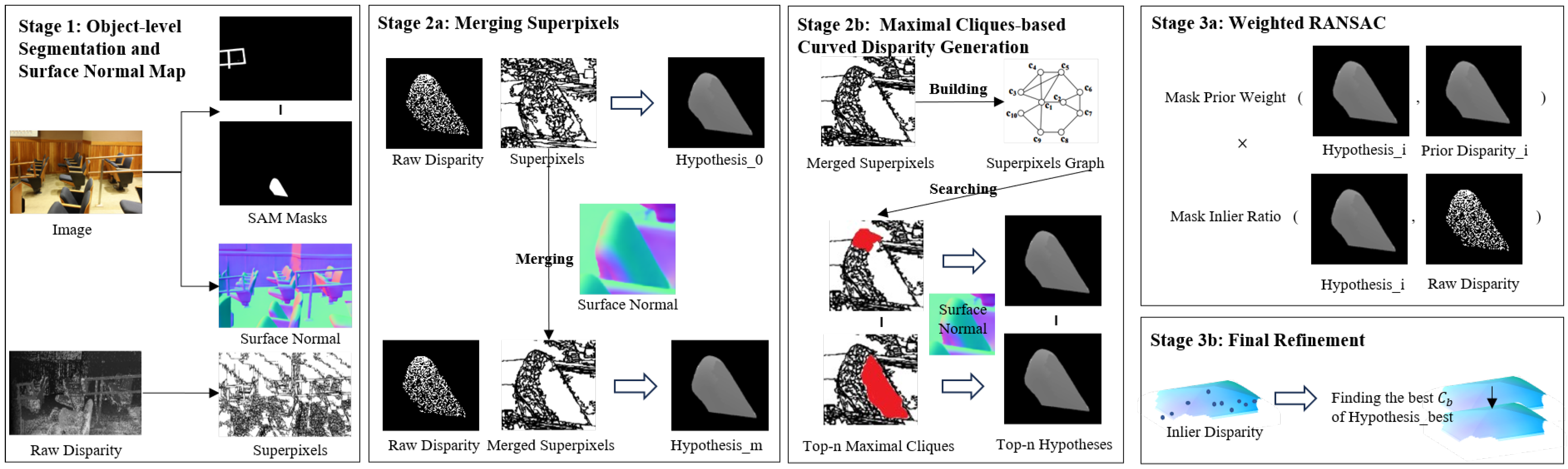
  • We refine a stereo matching pipeline with monocular vision models (zero-shot monocular surface normal prediction and SAM). The method can directly enhance the traditional disparity refinement methods and achieve state-of-the-art performance.
  • We build a new object-level weighted RANSAC framework based on SAM segmentation masks, which can balance disparity fitting and geometry structure similarity to prior geometry structure (monocular surface normal prediction).
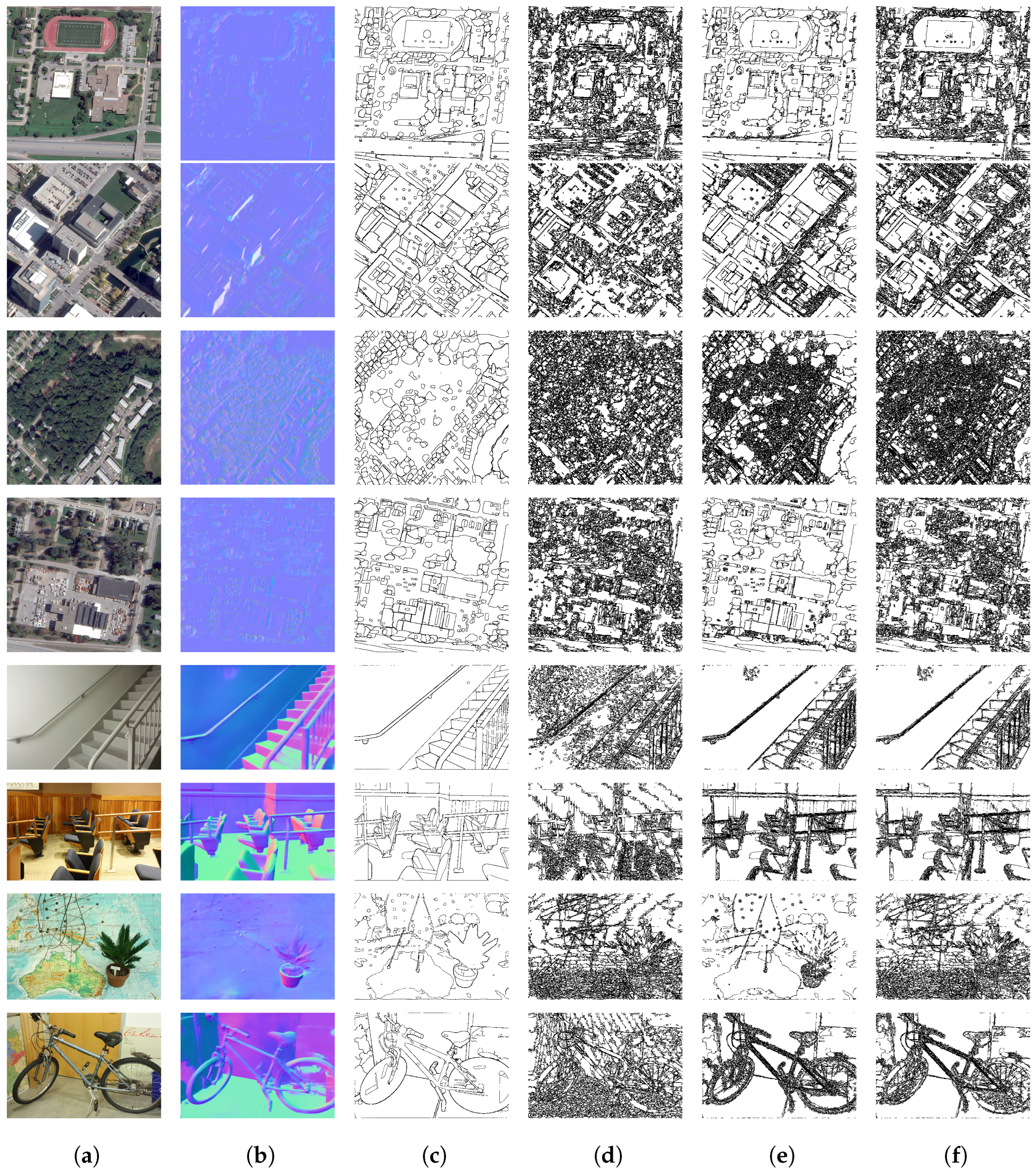
  • We utilize the SAM segmentations and surface normal prediction to obtain a better superpixel segmentation with large planes.
  • We use maximum cliques search to obtain superpixels with the correct disparity in SAM masks and build possible curved disparity hypotheses.

2. Related Works

2.1. Disparity Refinement in Traditional Stereo Pipelines

Refining the estimated disparity is usually considered the last step of traditional stereo pipelines [27], like local-means filtering [28] and some recent deep learning-based methods [27]. The algorithm similar to our method is another type of disparity refinement algorithms [29,30], which are directly based on deep learning cost volume or disparity map like SDR [20]. For remote sensing images, some works propose to refine the disparity in urban scenes based on open-source GIS data [31]. For these methods, the geometric structures’ information in 3D scenes is rarely considered in stereo matching or disparity refinement. Piece-wise smoothness is still a commonly used assumption. In this paper, we notice the curved surface and the bigger plane structure in scenes and introduce a SAM and prior normal-based new framework.

2.2. Disparity Refinement in End-to-End Neural Networks

In recent years, disparity refinement modules have appeared in a large number of dense matching neural networks [21,22]. These studies rely on image pairs with ground-truth disparity and conduct disparity estimation through end-to-end neural networks. They mainly use the disparity refinement modules to optimize small detail errors [22,32,33]. HITNet [21] does not explicitly build a volume and instead relies on a fast multiresolution disparity initialization step, differentiable 2D geometric propagation, and warping mechanisms to infer disparity hypotheses. Our viewpoint is that disparity refinement is a monocular vision problem as the last step of stereo pipelines. Disparity refinement modules in these end-to-end neural networks only utilize disparity without other annotation data. Pretrained monocular vision models are also rarely utilized to stereo matching neural networks. Many monocular vision models are trained with large datasets different from common stereo datasets [34] and have powerful performance.
We think stereo matching models can be complemented by monocular vision models. In this paper, the pre-trained SAM model and pre-trained monocular surface normal prediction neural network are used to refine a noisy disparity map on the condition of the zero-shot cross-dataset. The experimental results show that our framework can achieve competitive performance even based on the traditional RANSAC disparity refinement framework.

2.3. Normal Assisted Depth (Disparity) Estimation

Numerous methods have been proposed to estimate single view depth or stereo depth by the joint learning of normal and depth [19,35,36]. Although these methods have made some progress, it is still a key problem in the interactive utilization of normal and depth (disparity).
In work [37], normal information is used to guide the aggregation of the SGM algorithm, but their purpose is to make the SGM algorithm adapt to the slanted plane. The closest to our method is the CNN prediction normal-based algorithm [29]. However, they directly model the problem as a linear system of the whole disparity map and surface normal map, lacking the understanding of object patterns in normal maps. The understanding of scene geometry in their method all depends on the edge map. In this paper, we build a linear system of disparity and surface normal values at the object level assisted by SAM segmentations. We consider different disparity hypotheses, and the hypotheses are selected based on our weighted RANSAC method. The experimental results show that these geometric structures extracted based on normal can effectively help disparity refinement.

3. Rethinking Ransac-Based Disparity Refinement

Given an image I R H × W , we are interested in recovering the corresponding disparity map D when only a noisy and possibly incomplete estimate D ¯ is available.

3.1. Former Methods

Former RANSAC-based methods assume the scene structure to be piece-wise planar. Based on image superpixels segmentation g k , k = 1 , 2 , , M g , the disparity map is:
D = k = 1 M g π k ,
π k = a k u + b k v + c k , if ( u , v ) g k 0 , otherwise ,
where M g is the number of planes, ( a k , b k , c k ) is the parameter of plane π k , and ( u , v ) is the coordination of image I. The estimation of the disparity map can transform into the following RANSAC disparity map model fitting problem:
D = argmax D H ( u , v ) I f ( D ( u , v ) D ¯ ( u , v ) ) ,
f ( x ) = 1 , if | x | 1 0 , otherwise ,
where H is the whole disparity map hypothesis set. Since the disparity plane only relies on local disparity values, fitting the whole disparity map D is equal to fitting disparity plane π k independently. Disparity plane π k , k = 1 , 2 , , M g is fitted for each superpixel in superpixels g k .
However, refining the disparity map relying on the former method can be difficult. Under piece-wise planar assumption, the segmentations of the image must be small, or there will be errors in approximating the curved disparity surface with a plane. But  D ¯ can be noisy and possibly incomplete, as there are always not enough reliable disparity values of D ¯ within a small superpixel. Because we only maximize the inliers ratio of superpixels, these disparity planes will be fitted erroneously. The fitting error comes from segmentations, the disparity map model, and optimization function, especially in a real scene with a curved disparity map.
Therefore, ( u , v ) is the coordination of image I. To better recover the disparity map, three rules should be considered: (1) segmentations are appropriate such that every segmentation contains correct disparity values; (2) the algorithm can reconstruct a disparity surface with complex geometric structures (we possibly obtain non-planar segmentation when ensuring rule 1); and (3) maximizing the optimization problem can give a correct answer. Obviously, these issues cannot be handled by relying on the former methods.

3.2. Proposed Disparity Map Model and Optimization Equation

We assume the scene structure to be piece-wise curved. A real scene with curved disparity map D consists of M s surfaces S k :
D = k = 1 M s S k ,
S k = k = 1 N 1 k π k + l = 1 N 2 k π l m + s = 1 N 3 k ϕ s .
Here, M s is the number of disparity surfaces, π l m is the bigger plane, and ϕ s is the curved surface. For the k-th disparity surface, the best model is one of the three surface models π k , π l m , ϕ s or a combination of them. For example, if only π k are used, the curved disparity surface can be approximated by planes as former methods. Some small planes π k without enough reliable disparity should be components of a bigger plane π l m , or disparity plane fitting can be affected due to incorrect local disparity. In addition, some disparity surfaces need to be approximated by complex surfaces ϕ s if the piece-wise planar assumption does not work.
While estimating the disparity map, we don’t know which model is the best. So the estimation question is transformed into the following weighted RANSAC disparity map model fitting problem:
D = argmax D H ( u , v ) I w ( u , v ; D ) f ( D ( u , v ) D ¯ ( u , v ) ) .
Here, w ( u , v ; D ) is the weight to measure the similarity between proposal D and the true curved disparity surface at ( u , v ) . The final disparity map should balance disparity fitting and shape similarity. The former RANSAC-based methods are the special case of our framework. Firstly, they fit the disparity map only by small planes π k , neglecting bigger planes and curved surfaces. Secondly, the former methods choose w ( u , v ; D ) = 1 .

4. Disparity Fitting Based on SAM and Surface Normal

In our method, the above question is solved based on SAM segmentation and monocular surface normal prediction. Figure 1 is an overview of our method. Firstly, we obtain M s segmentation masks s k , k = 1 , 2 , , M s based on the pre-trained SAM model and predict the surface normal map based on a pre-trained neural network. Secondly, we propose a two-step progressive method based on a basic disparity map to generate the disparity map hypotheses. Then, we calculate the weights of all disparity map proposals and the inlier ratios. The final disparity map is selected based on Equation (8). Finally, we refine the chosen disparity map at the SAM mask level. The method is summarized in Algorithm 1:
S k = argmax S k H k w ( S k ) ˙ ( u , v ) s k f ( S k ( u , v ) D ¯ ( u , v ) ) .
Here, SAM segmentations are the minimum units for our RANSAC optimization. Weights encode the structure similarity between the SAM mask-based disparity hypotheses and true disparity structure. Our weights are the same for all pixels in the same SAM mask for every disparity hypothesis.
Algorithm 1 Weighted RANSAC-based disparity estimation.
Input: 
Image I, noisy disparity map D ¯
   1:
 Predict superpixels g i , i = 1 , 2 , , M g , SAM masks s k , k = 1 , 2 , , M s and surface normal map.
   2:
 Obtain disparity planes hypothesis and its SAM mask-based disparity set → D 0 , S k 0 , k = 1 , 2 , , M s
   3:
 Obtain merged superpixels g i m , i = 1 , 2 , , M m and obtain merged disparity planes hypothesis → D m , S k m , k = 1 , 2 , , M s (Section 4.2.1) k = 1 , 2 , , M s
   4:
 for all k = 1, 2, ⋯, Ms do
   5:
  Surface normal map transformation → disparity constraint map (Section 4.2.2)
   6:
  Build the k-th SAM mask graph, and reconstruct top-n maximal cliques-based disparity hypothesis → S k j , j = 1 , 2 , , n (Section 4.2.3)
   7:
  Calculate hypothesis weights and choose the best hypothesis in S k 0 , S k m S k j , j = 1 , 2 , , n based on Equation (8)
   8:
  Final disparity refinement
   9:
  Update disparity map D
 10:
 end for
Output: 
 Disparity map D

4.1. Object-Level Segmentation and Surface Normal Map

In our assumption, the disparity value is structurally constrained in its object-level segmentation. We obtain M segmentation masks based on the pre-trained SAM model automatically. It works by sampling single-point input prompts in a grid over the image, from each of which SAM can predict multiple masks. Then, the masks are filtered for quality and deduplicated using non-maximal suppression. In addition, we count the area of all masks and choose the mask with the smallest area as the final mask on each pixel position.
Superpixels are segmented by the graph-based segmentation [38]. Meanwhile, we predict the surface normal map based on image I. The surface normal map is used in the merging superpixels step, disparity map hypothesis generation step, and hypothesis weights calculating step.

4.2. Two-Step Hypothesis Generation

We use a two-step progressive method based on a basic disparity map to generate a disparity hypotheses set. A basic disparity map D 0 is generated based on a local segment-based disparity plane fitting. Here, we use the SDR algorithm. The SDR algorithm refines the disparity map based on fitting and optimizing over-segmented superpixels g k . Based on the SAM masks, we obtain the SAM mask disparity set S k 0 , k = 1 , 2 , , M s .
In the first step, we merge small superpixels into bigger segmentations based on SAM masks and the surface normal. The merged superpixel segmentations are used to generate disparity map D m based on the SDR algorithm. Then, we obtain S k m , k = 1 , 2 , , M s too. S k m consists of small disparity planes and merged bigger disparity planes.
In the second step, we search for the maximum cliques of superpixels in each SAM mask. Maximum cliques should be consistent with the predicted surface normal structure. For the j-th SAM mask, we choose the top-n maximum cliques. The n curved disparity map hypothesis S j n is generated to replace the noisy superpixels’ disparity. So S j n consists of small disparity planes, merged bigger disparity planes, and curved surfaces. The final disparity map hypothesis for the j-th SAM mask is S j 0 , S j m S j i , i = 1 , 2 , , n .

4.2.1. Merging Superpixels

We consider merging superpixels g k into superpixels g k m . Firstly, we estimate the mean disparities of superpixels like the SDR algorithm and merge the neighboring superpixels when their mean disparities are the same. Secondly, we estimate the mean disparity normal vectors of superpixels. For superpixels in the same SAM mask, we merge two superpixels based on the cosine distance:
N d = ( r , t ) μ s = μ t , | ν r · ν t | T 2 , ( r , t ) N ,
N n = ( r , t ) | ν r · ν t | T 1 ,
where N represents the set of neighboring superpixels. μ r is the mean disparity of superpixel r, and ν r is the normalized mean disparity normal vector of superpixel r. T 1 and T 2 are the distance threshold. T 2 is used to reject wrong plane merging. T 1 is used to merge non-connected superpixels. Here, T 1 = 0.999 and T 2 = 0.99 . We merge all neighboring superpixels in set N d N d and generate disparity map D m and S k m based on the SDR algorithm.

4.2.2. Surface Normal Transformation

We convert the predicted surface normal map to the disparity space as a prior structure constraint. The prior disparity normal map is used to generate disparity map hypotheses and calculate the weights of hypotheses in the following. Given the surface normal vector ( n x , n y , n z ) at pixel p, the tangent plane equation of the surface is represented as
n x x + n y y + n z z = h ,
where h encodes the plane’s unknown depth. In the pinhole model, 3D point ( x , y , z ) is projected into the camera image plane at pixel ( u , v ) :
u = x z f + u 0 , v = y z f + v 0 ,
where ( u 0 , v 0 ) are the coordinates of the camera principal point, and f are the focal lengths. Giving the baseline b, we obtain the local plane equation of pixel p:
D ( u , v ) = b n x h u + b n y h v + b ( f n z n x u 0 n y v 0 ) h .
For every pixel p, we calculate 3D point ( x , y , z ) and h based on the RANSAC fitted disparity map. So the surface normal vector ( n x , n y , n z ) is transformed to disparity normal vector ( n x d , n y d , n z d ) = ( b n x h , b n y h , b ( f n z n x u 0 n y v 0 ) h ) at every pixel p. The prior disparity normal vector is used to generate the disparity map hypotheses and calculate the weights of the hypotheses.

4.2.3. Maximal Cliques-Based Curved Disparity Generation

For each SAM mask, we aim to find superpixel cliques with correct disparity values and build disparity map hypotheses of the selected clique.
Here, our method is to select superpixel cliques that satisfy the prior disparity normal constraint. For the k-th SAM mask, we model the superpixels in the same mask as a graph. The edge weight between superoxide g r m and g t m is calculated as
d e ( r , t ) = e ( 1 ( d ( r , t ) ) 2 100 ) ,
d ( r , t ) = | S k m ( u t , v t ) S k m ( u r , v r ) L n x d d u + n y d d v | ,
where ( u r , v r ) and ( u t , v t ) are the center coordinate of superpixel g r m and g t m . L is a straight line from ( u r , v r ) to ( u t , v t ) .
We use the i g r a p h m a x i m a l c l i q u e s function in the igraph1 C++ library, which makes use of a modified Bron–Kerbosch algorithm [39]. We obtain the maximal set, sort all maximal cliques based on scores e N c N k · d e ( r , t ) and select the top-n maximal cliques. N c is the pixel number of the maximal clique, and N k is the pixel number of the whole SAM mask. d e ( r , t ) is the sum of the maximal clique’s edge weights. e N c N k is the spatial weight, which is used to screen for balanced areas of the maximal clique. Here, n = 5 .
We build the disparity map hypotheses of the selected clique based on the prior normal constraints and inlier disparity. For each pixel ( u , v ) , we have two prior normal constraint equations:
S k m ( u + 1 , v ) S k m ( u , v ) = n x d ( u , v ) ,
S k m ( u , v + 1 ) S k m ( u , v ) = n y d ( u , v ) .
So for a whole SAM mask’s bounding box with N k b pixels and normal constraints, we can construct a linear system as
A B d = n B d m ,
where A is a 2 N k b × N k b sparse matrix. n is a constraint vector. The normal constraints at the whole bounding box are used because SAM masks may consist of multiple disconnected regions. d m is an inlier disparity vector of S k m and B is the sparse weights matrix. We select pixels if | S k m ( u , v ) D ¯ ( u , v ) | < 0.2 and weight at pixel ( u , v ) are calculated by e | S k m ( u , v ) D ¯ ( u , v ) | . We obtain an estimated disparity vector d by solving the linear system. Considering the error of the prior normal map, we only accept surface reconstruction disparity if the superpixel’s inlier ratio is less than 0.3, and other disparity in the mask area is equal to S k m . The final hypotheses set of the k-th SAM mask is S k i , i = 1 , 2 , , n .

4.3. Weighted RANSAC and Final Refinement

The disparity hypotheses of each SAM mask are selected based on Equation (8). Weights encode the structure similarity between the SAM segment-based disparity hypotheses and prior disparity structure. For the k-th SAM mask, we calculate the weight of the hypothesis as
w ( S k ) = e min ( d r , t 1 ) t 2 ,
where S k is the input disparity hypothesis. d r measures the distance between the input disparity and the prior structure-based disparity. t 1 and t 2 are used to avoid small weights; t 1 = 13 and t 2 = 8 . For the maximal cliques-based disparity hypothesis, we choose a constant distance to measure the error of the prior normal map: d r = 0.25 . For S k 0 , S k m , we calculate the distance as
d r = 1 N k ( u , v ) s k | S k b ( u , v ) S k ( u , v ) | ,
where N k is the pixel number of the whole SAM mask. S k is the input disparity. S k b is the estimated disparity based on the above-mentioned linear system solver when the maximal clique is only the biggest superpixel. We select the best disparity map hypothesis in the hypotheses set S k 0 , S k m S k i , i = 1 , 2 , , 5 .
Finally, the selected SAM mask disparity hypothesis S k should be finally refined based on inlier pixels. We select pixels if | S k ( u , v ) D ¯ ( u , v ) | < 1 and obtain inlier pixels set s k i n l i e r . The final chosen SAM mask disparity is adjusted by bias C b as the following equation:
C b = argmin C b ( u , v ) s k i n l i e r ( S k ( u , v ) + C b D ¯ ( u , v ) ) 2 .

5. Experiments

5.1. Experiment Setup

The SAM model (downloaded from https://github.com/facebookresearch/segment-anything (accessed on 5 April 2023)) with the default model checkpoints are used in this paper. We use the default parameters for all images. The prior surface normal map is obtained based on method [40]. Here, we use the pre-trained model (downloaded from https://github.com/EPFL-VILAB/omnidata/tree/main (accessed on 16 March 2022)). The two networks are all trained on large-scale single-view datasets without using a common stereo dataset.
In terms of the SDR algorithm, we completely follow the setting recommended in their paper [20].

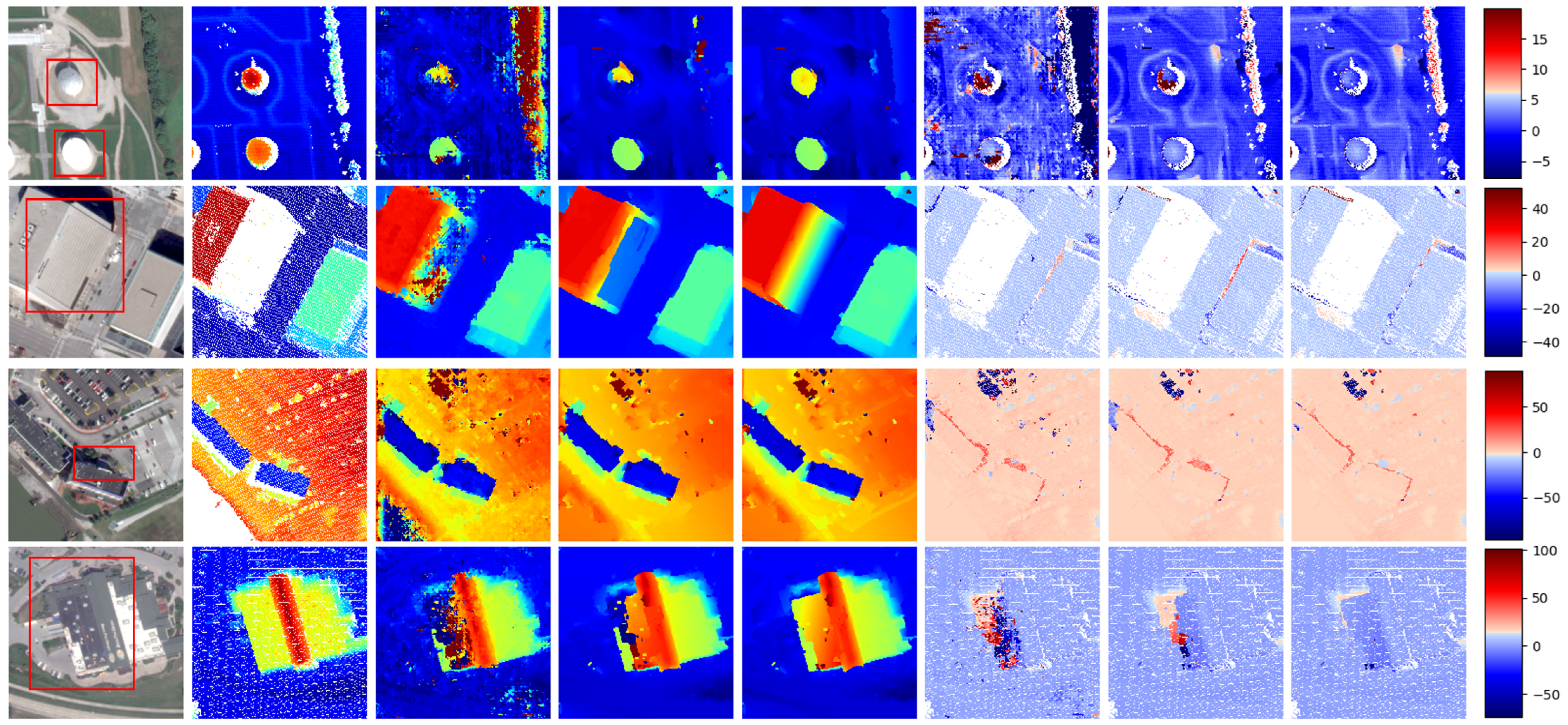
5.2. Experiments on US3D Benchmark

The US3D dataset provides 4292 RGB image pairs with publicly available ground-truth disparity maps. These images are collected from the WorldView-3 satellite, covering the United States cities of Jacksonville and Omaha, between 2014 and 2016. We chose Omaha as the testing set. We make comparisons with methods on the US3D dataset, including a commonly used traditional method SGM [9], disparity refinement model [20], and a deep learning-based method DenseMapNet [41].
We use the metrics from [42] to evaluate the performance of algorithms. To test the practicality of the algorithm, we adopt the proposed framework to optimize the results of the SGM algorithm. As shown in Table 1, the experimental results show that our proposed optimization framework enhances the average endpoint error (EPE) and the fraction of erroneous pixels (D1-error) of disparity maps compared to SGM and the original SDR. It should be noted that neither the selected segmentation model nor the surface normal prediction model are trained on remote sensing data. Compared with DenseMapNet trained on the US3D dataset, our framework still exhibits good performance without the need for training. This indicates that our algorithm provides a direct and effective approach to utilizing large-scale models.
Figure 2 shows the disparity map of SGM, SGM with SDR, SGM with our method, and the GT disparity map. As shown in the red circle, our method successfully reconstructs low-quality areas in the SGM disparity map by capturing SAM-based ground objects in satellite imagery and utilizing the structure provided by surface normal maps, resulting in a significant improvement compared to SDR. Figure 3 shows superpixel segmentations merging cases on the US3D Dataset. From left to right is the image, surface normal map, SAM segmentation edge map, superpixels edge map, our merged superpixels edge map, and the corresponding edge map of our final RANSAC selected hypothesis. Our method successfully merges superpixels into the maximum plane corresponding to the object. Our method can still maintain small segmentation in the curved surface region. For satellite imagery, our method can explore the planar structure of buildings such as roofs, while also avoiding the incorrect segmentation of curved areas such as vegetation.

5.3. Experiments on Middlebury Benchmark

We make comparisons with other state-of-the-art corresponding methods on the Middlebury stereo benchmark [43]. The dataset contains 30 image pairs, where 15 image pairs with the available disparity ground-truth are used for training while the other 15 image pairs are used for online evaluation. SDR uses the half-resolution dataset for evaluation, and we also follow this setting. Like SDR, the initial disparity map is generated by MC-CNN [13] with the winner-take-all method only. Our method can also optimize the results of deep learning models. We use the default error metric of the Middlebury dataset: bad 1.0 (%), bad 2.0 (%), bad 4.0 (%), avgerr (pixel), and rms (pixel).

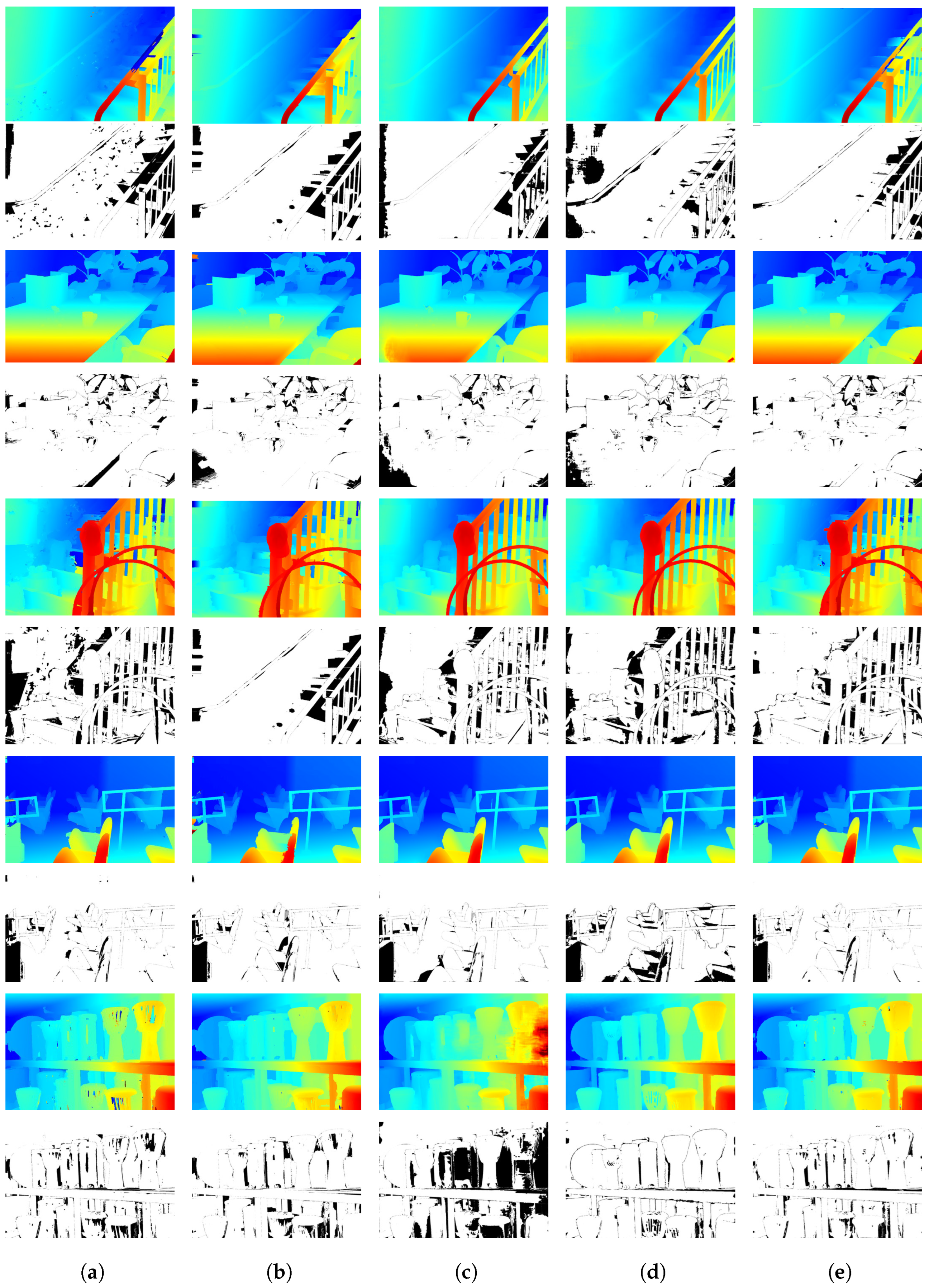
5.3.1. Comparison with Disparity Refinement Methods

Our approach is compared with the state-of-the-art disparity refinement methods SDR [20], MC-CNN+RBS [30], SNP-RSM [29], MC-CNN-acrt [13], SGM [9], MDP [44], and HITNet [21]. Here, SNP-RSM is a surface normal-based method. MDP refines an SGM disparity map. MC-CNN+RBS, MC-CNN-acrt, and SDR refine a disparity map of MC-CNN trained only on the Middlebury training dataset. HITNet is a learning-based state-of-the-art disparity refinement method. The results of five error metrics on the Middlebury dataset are listed in Table 2. Our framework and HITNet achieve competitive performance.
Compared with MC-CNN disparity map refinement methods, our framework outperforms them in all metrics. Especially for SDR, we use SDR as a basic plane fitting method in our framework. Our framework largely enhances the performance of SDR based on the understanding of structure. The reason is that we enhance segmentations for the whole scene. In our method, superpixels or SAM masks are not the right segmentations but a combination of them. Figure 3 shows superpixel segmentations merging cases on the Middlebury Benchmark of Staircase, Classroom2, Australia, and Bicycle2. From left to right is the image, surface normal map, SAM segmentation edge map, superpixels edge map, our merged superpixels edge map and the corresponding edge map of our final RANSAC selected hypothesis. Our method successfully merges superpixels into the maximum plane corresponding to the object. Our method can still maintain small segmentation in the curved surface region. For Australia and Bicycle2, SAM segmentations here are bad for catching details of small objects. Some merged superpixels are wrong, which leads to the error in disparity fitting. Our method compensates for such shortcomings by RANSAC hypotheses selecting.
For SNP-RSM, our framework outperforms SNP-RSM in all metrics. They directly model the problem as a linear system of the whole disparity and surface normal values, lacking the understanding of patterns in normal maps and objects. Especially for HITNet, the network is trained on SceneFlow and then fine-tuned on the Middlebury training images. We only use the MC-CNN initial disparity map which is trained only on the limited Middlebury training set. We do not use any matching algorithms. Our effect comes entirely from utilizing predicted SAM masks and surface normal structures to spread the correct disparity in the existing disparity maps. But we outperform HITNet in ‘bad 2.0’ and ‘bad 4.0’ metrics. This fully verifies the effectiveness of combining monocular models and stereo models. The disparity map and error map are shown in Figure 4. HITNet relies on the slanted plane hypothesis. The method cannot hold the big curved region on the DjembeL image pair in the last line of Figure 4. In high-curvature regions, the error of HITNET will make larger errors. Our method can obtain the structure from the surface normal prediction map to estimate the correct surface disparity. Also, SDR obtains the wrong disparity plane fitting results due to the noisy initial disparity map. Our method can maintain good performance on both planes and curved surfaces.

5.3.2. Comparison with Cost Volume-Based Hand-Crafted Methods

Our approach is also compared with the state-of-the-art cost volume-based hand-crafted methods PMSC [45], LocalExp [11], LESC [46] and HBP-ISP [12]. These methods are global optimization methods based on MC-CNN cost volume. As the result show in Table 2, our framework and HBP-ISP achieve competitive performance.
Some results of our framework and HBP-ISP are shown in Figure 4. Our method outperforms HBP-ISP in all metrics for these images cases. HBP-ISP is an image segmentation pyramid-based belief propagation method. As we can see, there are errors in the image segmentation pyramid or they do not utilize segmentation correctly, which causes some large area errors in the disparity map. Although they have segmentations based at different scales to capture objects of different scales, their segmentation-based method is still not good enough in some regions. For example, they cannot handle the large disparity plane, resulting in bad performance on Staircase, CrusadeP, and Hoops images’ walls or desktops. In addition, serious errors occur on some objects, such as the chair in the Classroom2 image. For our method, the right line of Figure 3 shows the corresponding edge maps of our final RANSAC-selected hypothesis. This shows that our segmentation can adapt to multiple scales objects. And the lower ’avgerr’ error and ’rms’ error also show that we have a lower matching error of the overall scene. Note that HBP-ISP uses the entire cost volume, but our method only optimizes disparity maps to achieve this competitive effect.

5.3.3. Comparison with Cross-Domain Stereo Networks

Our approach is also compared with the state-of-the-art cross-domain stereo networks. MSTR [47] is only trained on the SceneFlow dataset. AdaStereo [14] is trained on the SceneFlow dataset and uses only images on the Middlebury Benchmark. CroCo-Stereo [15] is a recently proposed pre-training-based method. Our method only requires the MC-CNN trained on a small dataset. SAM and surface normal models are not trained on stereo datasets. As the result shown in Table 2, our framework and CroCo-Stereo achieve competitive performance. This indirectly demonstrates the generalization ability of the monocular visual model (SAM and surface normal model).

5.3.4. Hand-Crafted Initial Disparity Maps

Our method is also evaluated on different initial disparity maps. The results of the experiments are presented in Table 3. In addition to the r200 algorithm-based disparity map which is computed by the Intel RealSense R200 stereo model algorithm, our algorithm can handle the OpenCV SGBM disparity map. The two methods are both hand-crafted methods without training. The SDR method can only enhance the performance under a rough evaluation. But we can refine the SGBM disparity map and R200 disparity map and achieve better performance.

5.4. Ablation Experiment

We provide ablation experiments on the Middlebury training set to evaluate the contribution of the proposed modules. We use the R200 disparity map as the baseline. R200+SDR refines the R200 disparity map using the SDR algorithm. R200+SDR(m) refines the R200 disparity map using the SDR algorithm and our merged superpixels. R200+P refines the R200 disparity map using our algorithm (only the two types of plane-based hypotheses) but without the maximal-cliques hypothesis and final refinement. R200+P+M(0.3,3) refines the R200 disparity map using our algorithm (top-3 maximal cliques and accept the disparity region when the inlier ratio is lower than 0.3) without final refinement. R200+P+M(0.3,3)+R is the full steps method. The results of the experiments are shown in Table 4. Compared with SDR and SDR(m), R200+P selects better segmentation (superpixels or merged superpixels) and achieves better performance. The inlier ratio determines the accepted area of the selected maximal-cliques hypotheses. Due to some error details or error structure in the surface normal map, if we accept all selected maximal-cliques hypotheses, the ‘bad 1.0’ error and ’bad 2.0’ error are much higher, although the ‘avgerr’ error and ’rms’ error are lower. In addition, as shown in the result, the maximal-cliques hypothesis numbers have little impact on the performance of the method. We tend to choose fewer computation times. We also test the performance of the model under different weight hyperparameter settings. In Equation (19), we use two hyperparameters t 1 and t 2 to control the rationality of the entire weight distribution. As shown in Table 5, the experimental results show that the hyperparameters are not sensitive. Therefore, the selected hyperparameters can handle different datasets robustly.

5.5. Generalization Test on More Unseen Dataset

We also demonstrate the more cross-domain adaptation capabilities of our method and compare them with other cross-domain trained methods. This simultaneously tests the generalization of the monocular visual model (SAM and surface normal model) and the robustness of our method. The KITTI 2015 test dataset [49] and PlantStereo test dataset [50] are used here. The KITTI 2015 test dataset contains 200 test image pairs of outdoor driving scenes. And the PlantStereo test dataset contains 232 plant image pairs (spinach, tomato, pepper, and pumpkin). As shown in Figure 5, our method is able to effectively generalize to different unseen datasets even using a hand-crafted method initial disparity map or cross-domain neural networks initial disparity map.

5.6. Efficiency

According to the modified Bron–Kerbosch algorithm, our weighted RANSAC method runs in time O ( d n 3 d 3 ) , n is equal to the number of SAM masks, and d is equal to the highest number of superpixels in a SAM mask. Our algorithm can find disparity maps that are better than those fitted based on the piece-wise planar assumption within a limited time.
We implement our framework in C++ and OpenCV on a PC with a 2.3 GHz CPU. The average running time of our method in the Middlebury testing dataset is 160 s, while the average running time of SDR is 15 s. This is due to excessive computation times when we reconstruct the surfaces of some large SAM masks ( large SAM mask size or large image size). Increased computation times are seen in the steps of calculating the RANSAC weights and maximal-cliques disparity hypotheses.

6. Discusion

Although our method has made some progress, there are still some shortcomings. First, our algorithm is not fast enough because it runs on the CPU. Second, our algorithm ensures the effectiveness of the theory, but it is still unable to compare with the most advanced deep learning model. This will limit the application of our algorithm. Nevertheless, the idea of combining monocular and binocular vision tasks can be well extended to end-to-end neural networks. In the next step, we will combine surface normal prediction, segmentation, and stereo matching to form a multi-task deep learning model. We believe that this is one of the effective ways to develop 3D tasks.

7. Conclusions

This paper proposed a framework that combines stereo matching models and advanced monocular vision models. We explore the RANSAC disparity refinement based on zero-shot monocular surface normal prediction and SAM segmentation masks. The disparity refinement problem is formulated as follows: extracting geometric structures, building disparity map hypotheses of the geometric structures, and selecting the hypothesis-based weighted RANSAC method. We believe that after obtaining geometry structures, even if there is only a part of the correct disparity in the geometry structure, the entire correct geometry structure can be reconstructed based on the prior geometry structure. Experiments on the US3D dataset and Middlebury dataset demonstrate the accuracy and robustness. The research helps to promote the development of scene and geometric structure understanding in stereo disparity estimation and the application of combining advanced large-scale monocular vision models with stereo matching methods. We will continue to study stereo matching neural networks based on more monocular vision models later.

Author Contributions

Conceptualization, H.S. and T.W.; methodology, H.S. and T.W.; software, H.S. and T.W.; validation, H.S. and T.W.; formal analysis, H.S. and T.W.; investigation, H.S. and T.W.; resources, H.S. and T.W.; data curation, H.S. and T.W.; writing—original draft preparation, H.S.; writing—review and editing, T.W.; visualization, H.S.; supervision, T.W.; project administration, T.W.; funding acquisition, T.W. All authors have read and agreed to the published version of the manuscript.

Funding

This research received no external funding.

Data Availability Statement

The data utilized in this study were primarily sourced from publicly accessible resources.

Conflicts of Interest

The authors declare no conflicts of interest.

References

  1. Seitz, S.; Curless, B.; Diebel, J.; Scharstein, D.; Szeliski, R. A Comparison and Evaluation of Multi-View Stereo Reconstruction Algorithms. In Proceedings of the 2006 IEEE Computer Society Conference on Computer Vision and Pattern Recognition (CVPR’06), New York, NY, USA, 17–22 June 2006; Volume 1, pp. 519–528. [Google Scholar] [CrossRef]
  2. Zhang, X.; Cao, X.; Yu, A.; Yu, W.; Li, Z.; Quan, Y. UAVStereo: A Multiple Resolution Dataset for Stereo Matching in UAV Scenarios. IEEE J. Sel. Top. Appl. Earth Obs. Remote Sens. 2023, 16, 2942–2953. [Google Scholar] [CrossRef]
  3. Geiger, A.; Lenz, P.; Urtasun, R. Are we ready for autonomous driving? The KITTI vision benchmark suite. In Proceedings of the 2012 IEEE Conference on Computer Vision and Pattern Recognition, Providence, RI, USA, 16–21 June 2012; pp. 3354–3361. [Google Scholar] [CrossRef]
  4. Park, J.H.; Park, H.W. Fast view interpolation of stereo images using image gradient and disparity triangulation. Signal Process. Image Commun. 2003, 18, 401–416. [Google Scholar] [CrossRef]
  5. Zhang, T.; Zhuang, Y.; Chen, H.; Wang, G.; Ge, L.; Chen, L.; Dong, H.; Li, L. Posterior Instance Injection Detector for Arbitrary-Oriented Object Detection from Optical Remote Sensing Imagery. IEEE Trans. Geosci. Remote. Sens. 2023, 61, 5623918. [Google Scholar] [CrossRef]
  6. Zhuang, Y.; Liu, Y.; Zhang, T.; Chen, L.; Chen, H.; Li, L. Heterogeneous Prototype Distillation with Support-Query Correlative Guidance for Few-Shot Remote Sensing Scene Classification. IEEE Trans. Geosci. Remote. Sens. 2024, 62, 5627918. [Google Scholar] [CrossRef]
  7. Wang, G.; Zhuang, Y.; Chen, H.; Liu, X.; Zhang, T.; Li, L.; Dong, S.; Sang, Q. FSoD-Net: Full-scale object detection from optical remote sensing imagery. IEEE Trans. Geosci. Remote Sens. 2021, 60, 5602918. [Google Scholar] [CrossRef]
  8. Zhuang, Y.; Liu, Y.; Zhang, T.; Chen, H. Contour modeling arbitrary-oriented ship detection from very high-resolution optical remote sensing imagery. IEEE Geosci. Remote Sens. Lett. 2023, 20, 6000805. [Google Scholar] [CrossRef]
  9. Hirschmuller, H. Stereo Processing by Semiglobal Matching and Mutual Information. IEEE Trans. Pattern Anal. Mach. Intell. 2008, 30, 328–341. [Google Scholar] [CrossRef]
  10. Michael Bleyer, C.R.; Rother, C. PatchMatch Stereo—Stereo Matching with Slanted Support Windows. In Proceedings of the British Machine Vision Conference, Dundee, UK, 29 August–2 September 2011; pp. 14.1–14.11. [Google Scholar] [CrossRef]
  11. Taniai, T.; Matsushita, Y.; Sato, Y.; Naemura, T. Continuous 3D Label Stereo Matching Using Local Expansion Moves. IEEE Trans. Pattern Anal. Mach. Intell. 2018, 40, 2725–2739. [Google Scholar] [CrossRef]
  12. Yan, T.; Yang, X.; Yang, G.; Zhao, Q. Hierarchical Belief Propagation on Image Segmentation Pyramid. IEEE Trans. Image Process. 2023, 32, 4432–4442. [Google Scholar] [CrossRef]
  13. Žbontar, J.; Lecun, Y. Stereo matching by training a convolutional neural network to compare image patches. J. Mach. Learn. Res. 2016, 17, 1–32. [Google Scholar]
  14. Song, X.; Yang, G.; Zhu, X.; Zhou, H.; Wang, Z.; Shi, J. AdaStereo: A Simple and Efficient Approach for Adaptive Stereo Matching. In Proceedings of the 2021 IEEE/CVF Conference on Computer Vision and Pattern Recognition (CVPR), Nashville, TN, USA, 19–25 June 2021; pp. 10323–10332. [Google Scholar] [CrossRef]
  15. Weinzaepfel, P.; Lucas, T.; Leroy, V.; Cabon, Y.; Arora, V.; Brégier, R.; Csurka, G.; Antsfeld, L.; Chidlovskii, B.; Revaud, J. CroCo v2: Improved Cross-view Completion Pre-training for Stereo Matching and Optical Flow. In Proceedings of the IEEE/CVF International Conference on Computer Vision (ICCV), Paris, France, 2–3 October 2023; pp. 17969–17980. [Google Scholar]
  16. Jiang, L.; Wang, F.; Zhang, W.; Li, P.; You, H.; Xiang, Y. Rethinking the Key Factors for the Generalization of Remote Sensing Stereo Matching Networks. IEEE J. Sel. Top. Appl. Earth Obs. Remote Sens. 2025, 18, 4936–4948. [Google Scholar] [CrossRef]
  17. Bae, G.; Budvytis, I.; Cipolla, R. IronDepth: Iterative Refinement of Single-View Depth using Surface Normal and its Uncertainty. In Proceedings of the 33rd British Machine Vision Conference 2022, BMVC 2022, London, UK, 21–24 November 2022. [Google Scholar]
  18. Qi, X.; Liao, R.; Liu, Z.; Urtasun, R.; Jia, J. GeoNet: Geometric Neural Network for Joint Depth and Surface Normal Estimation. In Proceedings of the 2018 IEEE/CVF Conference on Computer Vision and Pattern Recognition, Salt Lake City, UT, USA, 18–23 June 2018; pp. 283–291. [Google Scholar] [CrossRef]
  19. Rossi, M.; Gheche, M.E.; Kuhn, A.; Frossard, P. Joint Graph-Based Depth Refinement and Normal Estimation. In Proceedings of the IEEE/CVF Conference on Computer Vision and Pattern Recognition (CVPR), Seattle, WA, USA, 13–19 June 2020. [Google Scholar]
  20. Yan, T.; Gan, Y.; Xia, Z.; Zhao, Q. Segment-Based Disparity Refinement with Occlusion Handling for Stereo Matching. IEEE Trans. Image Process. 2019, 28, 3885–3897. [Google Scholar] [CrossRef] [PubMed]
  21. Tankovich, V.; Hane, C.; Zhang, Y.; Kowdle, A.; Fanello, S.; Bouaziz, S. HITNet: Hierarchical Iterative Tile Refinement Network for Real-time Stereo Matching. In Proceedings of the IEEE/CVF Conference on Computer Vision and Pattern Recognition (CVPR), Nashville, TN, USA, 20–25 June 2021; pp. 14362–14372. [Google Scholar]
  22. Lipson, L.; Teed, Z.; Deng, J. RAFT-Stereo: Multilevel Recurrent Field Transforms for Stereo Matching. In Proceedings of the 2021 International Conference on 3D Vision (3DV), Virtual, 1–3 December 2021; pp. 218–227. [Google Scholar] [CrossRef]
  23. Cheng, H.K.; Oh, S.W.; Price, B.; Schwing, A.; Lee, J.Y. Tracking Anything with Decoupled Video Segmentation. In Proceedings of the ICCV, Paris, France, 2–3 October 2023. [Google Scholar]
  24. Yu, T.; Feng, R.; Feng, R.; Liu, J.; Jin, X.; Zeng, W.; Chen, Z. Inpaint Anything: Segment Anything Meets Image Inpainting. arXiv 2023, arXiv:2304.06790. [Google Scholar]
  25. Gao, S.; Lin, Z.; Xie, X.; Zhou, P.; Cheng, M.M.; Yan, S. EditAnything: Empowering Unparalleled Flexibility in Image Editing and Generation. In Proceedings of the 31st ACM International Conference on Multimedia, Demo Track, Ottawa, ON, Canada, 29 October–3 November 2023. [Google Scholar]
  26. Kirillov, A.; Mintun, E.; Ravi, N.; Mao, H.; Rolland, C.; Gustafson, L.; Xiao, T.; Whitehead, S.; Berg, A.C.; Lo, W.Y.; et al. Segment Anything. arXiv 2023, arXiv:2304.02643. [Google Scholar]
  27. Aleotti, F.; Tosi, F.; Zama Ramirez, P.; Poggi, M.; Salti, S.; Di Stefano, L.; Mattoccia, S. Neural Disparity Refinement for Arbitrary Resolution Stereo. In Proceedings of the International Conference on 3D Vision, Virtual, 1–3 December 2021. [Google Scholar]
  28. Favaro, P. Recovering thin structures via nonlocal-means regularization with application to depth from defocus. In Proceedings of the 2010 IEEE Computer Society Conference on Computer Vision and Pattern Recognition, San Francisco, CA, USA, 13–18 June 2010; pp. 1133–1140. [Google Scholar] [CrossRef]
  29. Zhang, S.; Xie, W.; Zhang, G.; Bao, H.; Kaess, M. Robust stereo matching with surface normal prediction. In Proceedings of the 2017 IEEE International Conference on Robotics and Automation (ICRA), Singapore, 29 May–3 June 2017; pp. 2540–2547. [Google Scholar] [CrossRef]
  30. Barron, J.T.; Poole, B. The Fast Bilateral Solver. In Proceedings of the Computer Vision—ECCV 2016, Amsterdam, The Netherlands, 1–14 October 2016; pp. 617–632. [Google Scholar]
  31. Wang, X.; Jiang, L.; Wang, F.; You, H.; Xiang, Y. Disparity Refinement for Stereo Matching of High-Resolution Remote Sensing Images Based on GIS Data. Remote Sens. 2024, 16, 487. [Google Scholar] [CrossRef]
  32. Xu, G.; Wang, X.; Ding, X.; Yang, X. Iterative Geometry Encoding Volume for Stereo Matching. In Proceedings of the IEEE/CVF Conference on Computer Vision and Pattern Recognition, Vancouver, BC, Canada, 17–24 June 2023; pp. 21919–21928. [Google Scholar]
  33. Shen, Z.; Dai, Y.; Song, X.; Rao, Z.; Zhou, D.; Zhang, L. PCW-Net: Pyramid Combination and Warping Cost Volume for Stereo Matching. In Proceedings of the European Conference on Computer Vision, Tel Aviv, Israel, 23–27 October 2022; pp. 280–297. [Google Scholar]
  34. Dai, A.; Chang, A.X.; Savva, M.; Halber, M.; Funkhouser, T.; Nießner, M. ScanNet: Richly-annotated 3D Reconstructions of Indoor Scenes. In Proceedings of the Computer Vision and Pattern Recognition (CVPR), Honolulu, HI, USA, 21–26 July 2017. [Google Scholar]
  35. Dharmasiri, T.; Spek, A.; Drummond, T. Joint prediction of depths, normals and surface curvature from RGB images using CNNs. In Proceedings of the 2017 IEEE/RSJ International Conference on Intelligent Robots and Systems (IROS), Vancouver, BC, Canada, 24–28 September 2017; pp. 1505–1512. [Google Scholar]
  36. Yin, W.; Liu, Y.; Shen, C. Virtual Normal: Enforcing Geometric Constraints for Accurate and Robust Depth Prediction. IEEE Trans. Pattern Anal. Mach. Intell. 2022, 44, 7282–7295. [Google Scholar] [CrossRef]
  37. Scharstein, D.; Taniai, T.; Sinha, S.N. Semi-global Stereo Matching with Surface Orientation Priors. In Proceedings of the 2017 International Conference on 3D Vision (3DV), Qingdao, China, 10–12 October 2017; pp. 215–224. [Google Scholar] [CrossRef]
  38. Felzenszwalb, P.F.; Huttenlocher, D.P. Efficient graph-based image segmentation. Int. J. Comput. Vis. 2004, 59, 167–181. [Google Scholar] [CrossRef]
  39. Eppstein, D.; Löffler, M.; Strash, D. Listing All Maximal Cliques in Sparse Graphs in Near-Optimal Time. In Algorithms and Computation; Cheong, O., Chwa, K.Y., Park, K., Eds.; Springer: Berlin/Heidelberg, Germany, 2010; pp. 403–414. [Google Scholar]
  40. Eftekhar, A.; Sax, A.; Malik, J.; Zamir, A. Omnidata: A Scalable Pipeline for Making Multi-Task Mid-Level Vision Datasets From 3D Scans. In Proceedings of the IEEE/CVF International Conference on Computer Vision, Montreal, QC, Canada, 10–17 October 2021; pp. 10786–10796. [Google Scholar]
  41. Atienza, R. Fast disparity estimation using dense networks. In Proceedings of the 2018 IEEE International Conference on Robotics and Automation (ICRA), Brisbane, Australia, 12–25 May 2018; pp. 3207–3212. [Google Scholar]
  42. He, S.; Li, S.; Jiang, S.; Jiang, W. HMSM-Net: Hierarchical multi-scale matching network for disparity estimation of high-resolution satellite stereo images. ISPRS J. Photogramm. Remote Sens. 2022, 188, 314–330. [Google Scholar] [CrossRef]
  43. Scharstein, D.; Hirschmüller, H.; Kitajima, Y.; Krathwohl, G.; Nešić, N.; Wang, X.; Westling, P. High-Resolution Stereo Datasets with Subpixel-Accurate Ground Truth. In Pattern Recognition; Jiang, X., Hornegger, J., Koch, R., Eds.; Springer: Cham, Switzerland, 2014; pp. 31–42. [Google Scholar]
  44. Li, A.; Chen, D.; Liu, Y.; Yuan, Z. Coordinating Multiple Disparity Proposals for Stereo Computation. In Proceedings of the 2016 IEEE Conference on Computer Vision and Pattern Recognition (CVPR), Las Vegas, NV, USA, 27–30 June 2016; pp. 4022–4030. [Google Scholar] [CrossRef]
  45. Li, L.; Zhang, S.; Yu, X.; Zhang, L. PMSC: PatchMatch-Based Superpixel Cut for Accurate Stereo Matching. IEEE Trans. Circuits Syst. Video Technol. 2018, 28, 679–692. [Google Scholar] [CrossRef]
  46. Cheng, X.; Zhao, Y.; Yang, W.; Hu, Z.; Yu, X.; Sang, H.; Zhang, G. LESC: Superpixel cut-based local expansion for accurate stereo matching. IET Image Process. 2022, 16, 470–484. [Google Scholar] [CrossRef]
  47. Guo, W.; Li, Z.; Yang, Y.; Wang, Z.; Taylor, R.H.; Unberath, M.; Yuille, A.; Li, Y. Context-Enhanced Stereo Transformer. In Proceedings of the Computer Vision—ECCV 2022, Tel Aviv, Israel, 23–27 October 2022; Avidan, S., Brostow, G., Cissé, M., Farinella, G.M., Hassner, T., Eds.; Springer: Cham, Switzerland, 2022; pp. 263–279. [Google Scholar]
  48. Keselman, L.; Iselin Woodfill, J.; Grunnet-Jepsen, A.; Bhowmik, A. Intel RealSense Stereoscopic Depth Cameras. In Proceedings of the IEEE Conference on Computer Vision and Pattern Recognition (CVPR) Workshops, Honolulu, HI, USA, 21–26 July 2017. [Google Scholar]
  49. Menze, M.; Geiger, A. Object Scene Flow for Autonomous Vehicles. In Proceedings of the Conference on Computer Vision and Pattern Recognition (CVPR), Boston, MA, USA, 7–12 June 2015. [Google Scholar]
  50. Wang, Q.; Wu, D.; Liu, W.; Lou, M.; Jiang, H.; Ying, Y.; Zhou, M. PlantStereo: A High Quality Stereo Matching Dataset for Plant Reconstruction. Agriculture 2023, 13, 330. [Google Scholar] [CrossRef]
Figure 1. An overview of our method. In the first stage, we obtain SAM masks, superpixels, and surface normal maps. In the second stage, we use a two-step progressive method based on a basic disparity map to generate a disparity hypothesis set. In the final stage, we select the best hypothesis for each SAM mask based on weighted RANSAC and refine them.
Remotesensing 17 01587 g001
Figure 2. Visualization examples of US3D. Left to right: left views, GT disparity map, SGM, SGM with SDR, SGM with our method, error map of SGM, error map of SDR, and error map of our method. As shown in the red box, our method successfully reconstructs low-quality areas in the SGM disparity map by capturing SAM-based ground objects in satellite imagery and utilizing the structure provided by surface normal maps, resulting in a significant improvement compared to SDR.
Remotesensing 17 01587 g002
Figure 3. Superpixel segmentation merging cases on the US3D Dataset and Middlebury Benchmark of Staircase, Classroom2, Australia and Bicycle2. (af) Reference image, surface normal map, SAM segmentation edge map, superpixels edge map, our merged superpixels edge map and the corresponding edge map of our final RANSAC selected hypothesis. Our method successfully merges superpixels into the maximum plane corresponding to the object. Our method can still maintain small segmentation in the curved surface region. For satellite imagery, our method can explore the planar structure of buildings such as roofs, while also avoiding incorrect segmentation of curved areas such as vegetation. For Australia and Bicycle2, SAM segmentations here are bad for catching the details of small objects. Some merged superpixels are wrong, which leads to the error in disparity fitting. Our method compensates for such shortcomings by RANSAC hypothesis selecting.
Remotesensing 17 01587 g003
Figure 4. Qualitative comparison on the Middlebury Benchmark testing images. From top to bottom is the disparity map and bad 4.0 error map of Staircase, CrusadeP, Hoops, and Classroom2. (ae) The different methods: SDR, HBP-ISP, HITNet, AdaStereo and our method. Our method has good performance in the curved surface region and the big plane region.
Remotesensing 17 01587 g004
Figure 5. Generalization cases on the unseen PlantStereo testing dataset and KITTI 2015 testing dataset. (af) Reference image, surface normal map, the corresponding edge map of our final RANSAC selected hypothesis, disparity of PSMNet, initial disparity, and our refinement results.
Remotesensing 17 01587 g005
Table 1. The US3D testing set. Quantitative comparison to our framework with different methods.
MethodEPE (Pixel)D1-Error (%)
SGM [9] 4.044 22.79
DenseMapNet [41]2.030 17.37
SGM + SDR [20] 2.257 16.44
SGM + ours 2.189 15.48
Table 2. The Middlebury Benchmark testing set. Quantitative comparison to state-of-the-art methods.
TypesMethodsBad 1.0Bad 2.0Bad 4.0AvgerrRms
NocAllNocAllNocAllNocAllNocAll
Surface Normal-
based Methods
SNP-RSM [29] 18.0 26.3 8.08 16.6 4.95 11.4 2.73 7.63 15.6 30.4
MC-CNN+ours 15.3 21.3 6.09 11.7 3.65 8.37 2.00 4.99 11.3 20.5
Refinement-based
Methods
SGM [9] 28.2 34.8 17.6 24.0 12.1 17.6 4.83 7.62 15.9 21.2
SGM+MDP [44] 18.1 27.5 8.42 18.1 5.08 13.9 2.67 8.19 15.0 29.9
MC-CNN-acrt [13] 17.1 27.3 8.75 19.1 4.91 15.8 3.82 17.9 21.3 55.0
MC-CNN+RBS [30] 18.1 27.5 8.42 18.1 5.08 13.9 2.67 8.19 15.0 29.9
MC-CNN+SDR [20] 18.8 25.1 7.69 13.8 4.90 10.0 2.94 6.16 15.4 24.2
HITNet [21] 13.3 20.7 6.46 12.8 3.81 8.66 1.71 3.29 9.97 14.5
MC-CNN+ours 15.3 21.3 6.09 11.7 3.65 8.37 2.00 4.99 11.3 20.5
Hand-crafted
SOTA Methods
PMSC [45] 14.8 22.8 6.71 13.6 4.44 9.71 2.26 5.65 12.9 23.9
LocalExp [11] 13.9 21.0 5.43 11.7 3.69 8.83 2.24 5.13 13.4 21.1
LESC [46] 16.7 23.1 6.78 12.8 4.48 9.38 2.58 5.33 14.5 21.7
HBP-ISP [12] 15.0 21.5 5.20 11.3 3.31 8.52 2.24 5.57 13.3 22.5
MC-CNN+ours 15.3 21.3 6.09 11.7 3.65 8.37 2.00 4.99 11.3 20.5
Cross-domain
Stereo Networks
MSTR [47] 21.6 32.0 8.72 20.7 3.99 16.4 2.19 21.6 13.8 61.8
AdaStereo [14] 29.5 35.5 13.7 19.8 6.35 10.9 2.22 3.39 10.2 12.9
CroCo-Stereo [15] 16.9 21.6 7.29 11.1 4.18 6.75 1.76 2.36 8.91 10.6
MC-CNN+ours 15.3 21.3 6.09 11.7 3.65 8.37 2.00 4.99 11.3 20.5
Table 3. The Middlebury training set. Quantitative comparison to our framework with different initial disparity maps.
MethodsBad 1.0Bad 2.0Bad 4.0AvgerrRms
NocAllNocAllNocAllNocAllNocAll
SGBM 34.3 41.4 23.3 30.9 17.7 25.3 8.37 16.2 25.3 42.0
SGBM+SDR 51.2 55.4 25.5 31.6 16.0 22.0 8.17 14.0 24.5 38.4
SGBM+ours 41.4 43.3 21.8 27.4 14.1 18.9 6.31 9.86 19.0 28.5
R200 [48] 42.0 49.4 34.3 42.5 30.4 38.9 23.1 31.9 53.8 64.5
R200+SDR 57.4 61.1 24.4 30.8 15.8 22.5 13.0 19.6 35.4 48.3
R200+ours [48] 39.7 45.1 20.8 27.0 15.0 20.8 8.67 14.0 24.9 36.9
Table 4. The Middlebury training set. Quantitative comparison to our framework with different setup.
MethodsBad 1.0Bad 2.0Bad 4.0AvgerrRms
NocAllNocAllNocAllNocAllNocAll
R200 42.0 49.4 34.3 42.5 30.4 38.9 23.1 31.9 53.8 64.5
R200+SDR 57.4 61.1 24.4 30.8 15.8 22.5 13.0 19.6 23.4 48.3
R200+SDR (m) 61.2 64.2 28.5 33.9 19.2 24.4 8.32 12.1 21.6 29.8
R200+P 57.5 61.1 23.2 29.2 14.8 20.7 8.62 14.1 24.0 36.6
R200+P+M (0.3,5) 57.3 60.7 22.9 28.8 14.4 20.0 8.23 13.5 23.5 35.8
R200+P+M (1.0,5)+R 52.1 56.2 22.1 28.2 14.7 20.5 8.49 13.8 23.9 36.4
R200+P+M (0.3,10)+R 40.0 45.2 20.2 26.2 14.2 19.9 7.99 13.3 23.5 35.8
R200+P+M (0.3,5)+R 39.7 45.1 20.8 27.0 15.0 20.8 8.67 14.0 24.9 36.9
Table 5. The Middlebury training set. Quantitative comparison to different weights setup.
MethodsBad 1.0Bad 2.0Bad 4.0AvgerrRms
NocAllNocAllNocAllNocAllNocAll
R200 42.0 49.4 34.3 42.5 30.4 38.9 23.1 31.9 53.8 64.5
R200+SDR 57.4 61.1 24.4 30.8 15.8 22.5 13.0 19.6 23.4 48.3
t 1 = 10 , t 2 = 8 40.1 45.2 20.3 26.3 14.5 20.0 8.17 13.9 25.1 36.7
t 1 = 16 , t 2 = 8 40.1 45.6 20.7 26.7 15.0 20.1 8.05 13.6 24.6 36.3
t 1 = 13 , t 2 = 4 41.2 46.0 21.2 27.6 15.2 21.1 8.15 13.4 24.1 36.1
t 1 = 13 , t 2 = 12 41.2 46.1 21.2 27.6 15.3 21.2 8.15 13.4 24.1 36.1
t 1 = 13 , t 2 = 8 40.0 45.2 20.2 26.2 14.2 19.9 7.99 13.3 23.5 35.8
Disclaimer/Publisher’s Note: The statements, opinions and data contained in all publications are solely those of the individual author(s) and contributor(s) and not of MDPI and/or the editor(s). MDPI and/or the editor(s) disclaim responsibility for any injury to people or property resulting from any ideas, methods, instructions or products referred to in the content.

