Article

SCF-CIL: A Multi-Stage Regularization-Based SAR Class-Incremental Learning Method Fused with Electromagnetic Scattering Features

1
The School of Electronic Engineering, Xidian University, Xi’an 710071, China
2
The Dipartimento di Ingegneria, University of Naples Parthenope, 80143 Naples, Italy
3
The National Laboratory of Radar Signal Processing, Xidian University, Xi’an 710071, China
4
The Academy of Advanced Interdisciplinary Research, Xidian University, Xi’an 710071, China
5
The National Inter-University Consortium for Telecommunications, 43124 Parma, Italy
*
Author to whom correspondence should be addressed.
Remote Sens. 2025, 17(9), 1586; https://doi.org/10.3390/rs17091586
Submission received: 15 January 2025 / Revised: 14 April 2025 / Accepted: 17 April 2025 / Published: 30 April 2025
(This article belongs to the Special Issue Recent Advances in SAR: Signal Processing and Target Recognition)

Abstract

:
Synthetic aperture radar (SAR) recognition systems often need to collect new data and update the network accordingly. However, the network faces the challenge of catastrophic forgetting, where previously learned knowledge might be lost during the incremental learning of new data. To improve the applicability and sustainability of SAR target classification methods, we propose a multi-stage regularization-based class-incremental learning (CIL) method for SAR targets, called SCF-CIL, which addresses catastrophic forgetting. This method offers three main contributions. First, for the feature extractor, we fuse the convolutional neural network features with the scattering center features using a cross-attention feature fusion structure, ensuring both the plasticity and stability of the extracted features. Next, an overfitting training strategy is applied to provide clustering space for unseen classes with an acceptable trade-off in the accuracy of the current classes. Finally, we analyze the influence of training with imbalanced data on the last fully connected layer and introduce a multi-stage regularization method by dividing the calculation of the fully connected layer into three parts and applying regularization to each. Our experiments on SAR datasets demonstrate the effectiveness of these improvements.

Graphical Abstract

1. Introduction

With the advantages of synthetic aperture radar (SAR), including all-day, all-weather, and long operation range [1], it is widely used to identify and monitor targets of concern [2,3,4]. In this domain, SAR target recognition methods aim to automatically identify the target within the image patch. To date, deep learning has demonstrated its remarkable capabilities in image processing applications [4], owing to its exceptional learning performance. With the development of deep learning, the application of deep neural networks (DNNs) in remote sensing target recognition is becoming increasingly popular [5,6,7,8,9,10,11]. These recognition methods realize outstanding performance in SAR target recognition on some pre-constructed fixed dataset.
However, in some certain application scenarios for SAR target classification, the radar system needs to continuously update the network’s functionality with newly collected data. The traditional network-based target recognition methods are fixed after training. When the network is adjusted using only newly collected data, it may suffer from catastrophic forgetting [12,13,14]; in other words, the network might forget the previously learned knowledge while training on the new data. To maintain recognition performance on the old classes, the entire network needs to be retrained with all the data whenever new data are acquired. However, storing all the data and retraining the network is storage-consuming, time-consuming, and computationally expensive. Therefore, standard conventional classification methods struggle to meet the demands of applications requiring continuous learning of new categories. In contrast, class-incremental learning (CIL) methods enable the model to progressively obtain new recognition abilities by processing new data arriving in batches, while retaining previously learned knowledge. This approach is well-suited for addressing the problem mentioned above [15,16,17,18]. Therefore, to improve the applicability and sustainability of SAR target classification methods, this paper focuses on applying CIL methods to SAR targets.
Figure 1 illustrates the main process of CIL. At stage i , the network is able to distinguish the instances of classes 1~ n 1 , where n = s i + 1 . Then, at stage i + 1 , the training data in stage i + 1 with s i + 1 classes are collected for network updating. The CIL method requires the network to recognize the new classes while retaining the ability to recognize the former n 1 classes. One thing to note is that the network usually does not have access to all the former data, for which there is a serious sample imbalance problem when training the network. Facing this problem, directly expanding the dimension of the classifier to increase the number of network classifier categories causes the network to tend to recognize the instances of the former classes as those of the current classes after training—in other words, forgetting the knowledge of the former classes, a phenomenon known as catastrophic forgetting [12,13]. This problem was first described by McCloskey and Cohen [14], who systematically analyzed the catastrophic interference in sequential learning scenarios.
To solve the problem of catastrophic forgetting in CIL, many researchers have made numerous efforts. iCaRL [19] calculated the average feature vectors for new and former classes using all instances of the new classes and a subset of instances from the former classes. It performed classification using the Nearest-Mean-of-Exemplars method, which minimized the parameters updated during the CIL process. Combining classification loss and distillation loss, iCaRL can release the influence caused by catastrophic forgetting. However, iCaRL tends to be overfitting to the former classes. To solve this problem, GEM [20] realized incremental learning by modifying the updating gradient direction of the current model. PackNet [21] iterated the process of training, pruning, and retraining to incrementally learning tasks. However, PackNet needs to manually adjust the pruning rate for different tasks, and due to limited network parameters, its task capacity is also limited. HAT [22] utilized a hard attention mask to keep part of the parameters unchanged and used the rest to learn new tasks. HAT is robust to different hyperparameter choices and has no limit on the number of total tasks.
Typical CIL networks can generally be divided into a feature extractor and a classifier, as shown in Figure 1. In the CIL process, the two structures collaborate to learn new knowledge while maintaining old knowledge. Specifically, the extractor should be able to extract the feature with enough completeness to distinguish classes beyond the known classes. Meanwhile, the classifier needs to maintain the ability to classify the former classes when trained with the data from current classes. When the CIL method tries to preserve the previous knowledge (i.e., stability), it often does so at the expense of reducing the method’s ability to learn new knowledge (i.e., plasticity) [23]. Based on the distinct roles of these two structures in the classification algorithm, this paper explores achieving a balance between plasticity and stability in the feature extractor and classifier, respectively.
In the above methods, most of them focus on optical image datasets [24]. However, SAR datasets exhibit substantial disparities compared to optical datasets, which causes a performance decrease when directly applying commonly used CIL methods to SAR datasets. The SAR image of the same target is significantly different as the depression angle changes, placing higher requirements on data feature extraction in the CIL process. In addition, SAR data have narrower frequency bandwidths, whereas optical imagery spans multiple spectral bands, rendering optical images rich in information, unlike SAR images which are comparatively less informative. Last but not least, complex SAR echo data contain lots of target information, such as target component information. Directly converting SAR echo data to visualized SAR images will result in the loss of a large amount of target information, which also makes it difficult for the CIL performance to reach the expected level.
Li et al. [25] mentioned that a robust and well-generalized representation of the training sample could increase the performance of the CIL algorithm, while SAR data contains rich target information that can be utilized. Many efforts have been made to extract and fuse SAR target features for classification. Park et al. [26] proposed a new size-related feature that is helpful for classifying tactical ground targets in a high-resolution SAR image. Clemente et al. [27] utilized the discrete-defined Krawtchouk moments to represent the military targets, which can realize robust classification with few features. Kang et al. [28] proposed a stacked autoencoder (SAE) to fuse 23 baseline features and a three-patch local binary pattern feature, which made the fused features more distinguishable and realizes better classification performance. Ding et al. [29] fused the global and local features for SAR automatic target recognition under extended operation conditions. Inspired by the above methods, this paper aims to explore a feature fusion method to effectively utilize the electromagnetic information, improving the CIL performance on SAR targets.
Based on the above discussion, our SCF-CIL method is proposed as shown in Figure 2. There are three main tasks for our method, two for the extractor and one for the classifier. One task of our feature extractor is to utilize the unique electromagnetic information contained in SAR data to improve the performance of our CIL method on SAR targets, while balancing the stability of SAR electromagnetic information with the plasticity of CNN features. The second task of the feature extractor is to provide clustering space for unseen classes. The classifier is required to achieve fair classification when training without the former class data.
In summary, this work makes three main contributions:
(1)
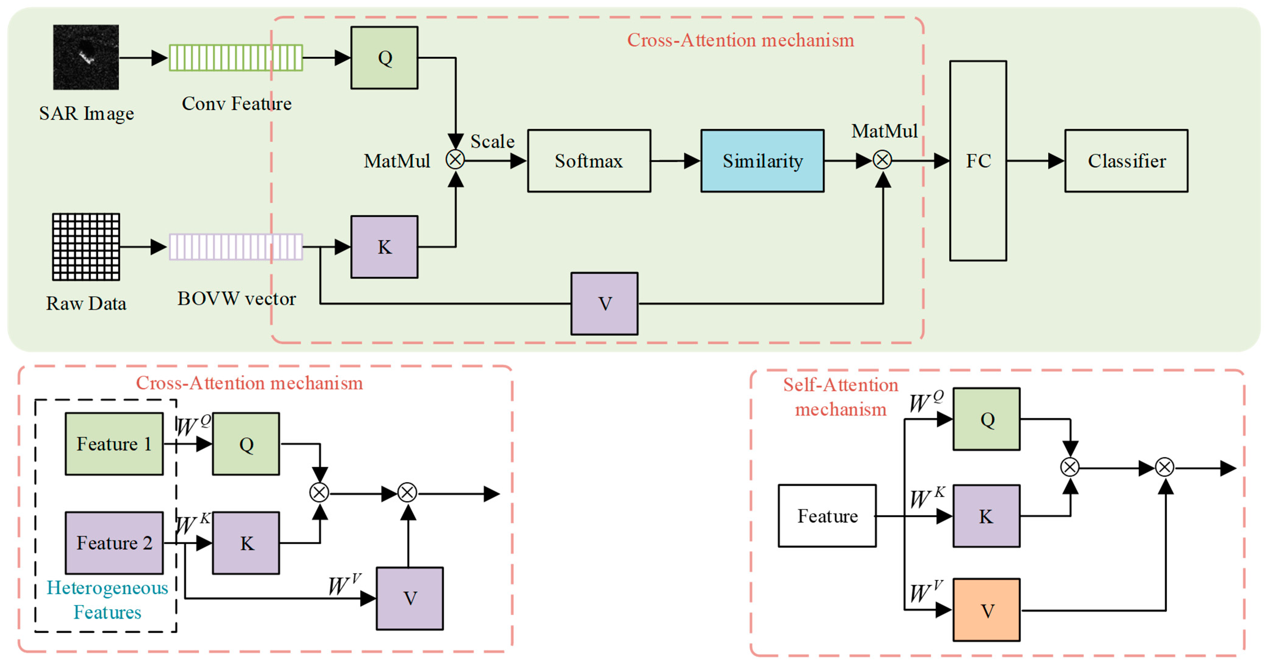
To make full use of the information contained in SAR echo data and to generalize a more balanced feature representation in terms of stability and plasticity, a feature fusion network, called SCF-Net, is proposed. First of all, the VGG16 [30] network is modified as a CNN feature extractor to extract the image feature. Meanwhile, we apply the bag of visual words (BOVW) model—originally proposed in [31,32] and recently applied to scattering feature transformation in [33]—to convert the electromagnetic attributed scattering center feature (SC feature) into a feature vector. Inspired by the effects of the attention mechanism on information processing, we utilize the cross-attention architecture to fuse the SC feature and CNN feature, and by integrating the stable inherent electromagnetic characteristics with plastic CNN feature, a more balanced representation in terms of stability and plasticity is generated.
(2)
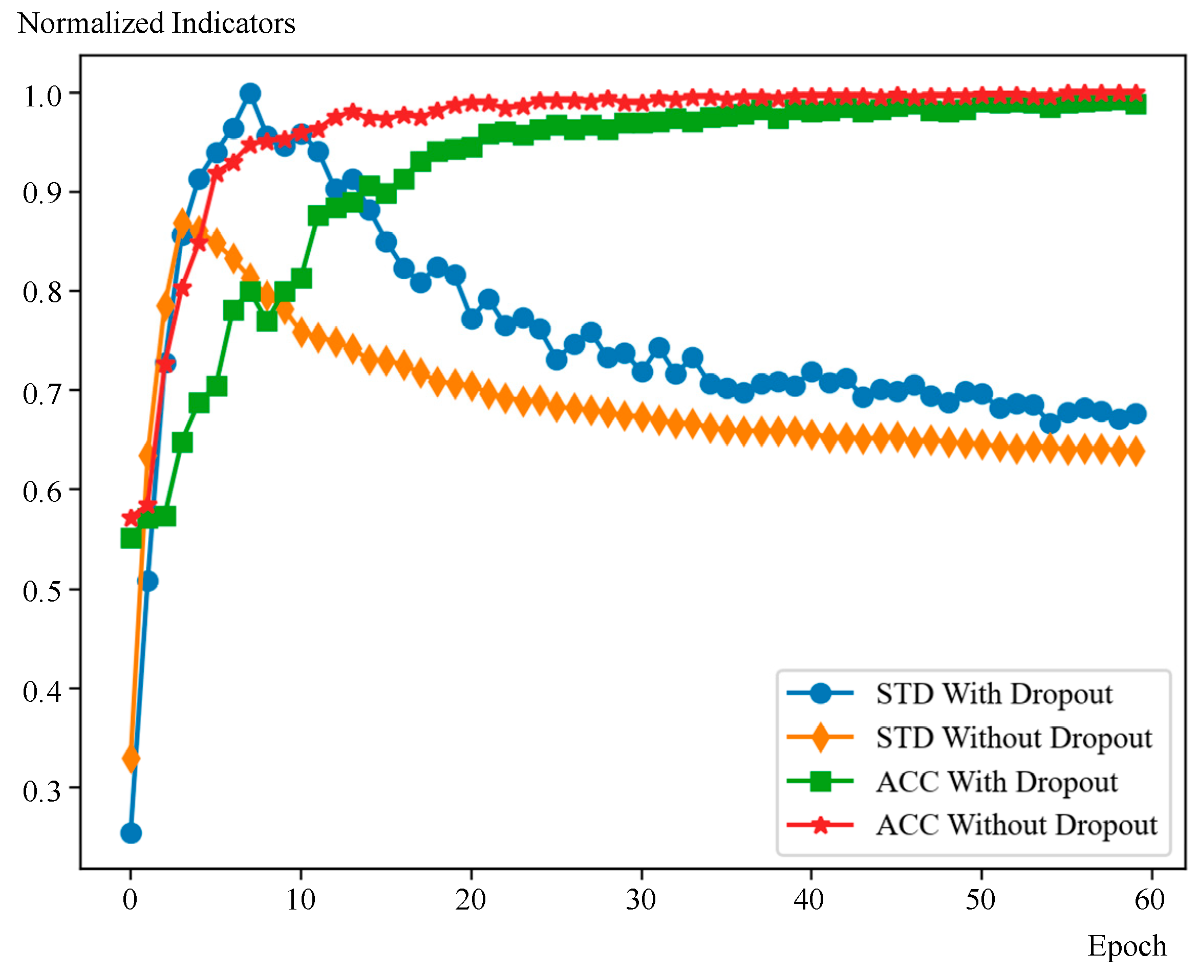
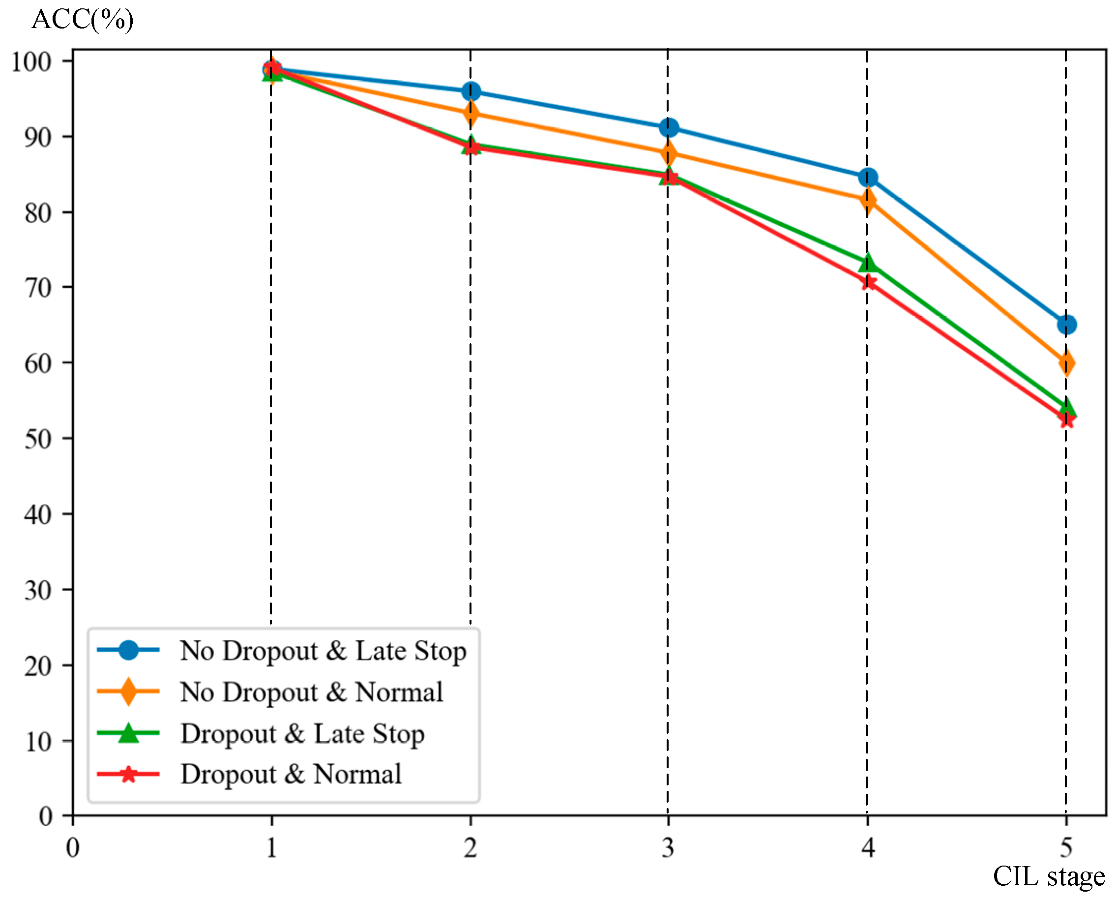
Analyzing the feature clustering in feature space, this paper concludes that an appropriate degree of overfitting could improve the performance of CIL in our specific model setting. Researchers always try to avoid overfitting in network training to improve the performance. However, for our feature that is fused with the stable SC feature, slight overfitting can make the features of the current classes to cluster more tightly in feature space, thereby improving classification performance when new classes are added, albeit at the cost of a slight decrease in recognition accuracy. According to this conclusion, two measures are applied, including removing the dropout structure and applying the “late-stop” strategy. By improving the feature clustering degree, our training strategy can reduce the probability that features of former classes fall into the new class subspace when trained with newly arrived data. This is another improvement in our optimization of the balance between plasticity and stability.
(3)
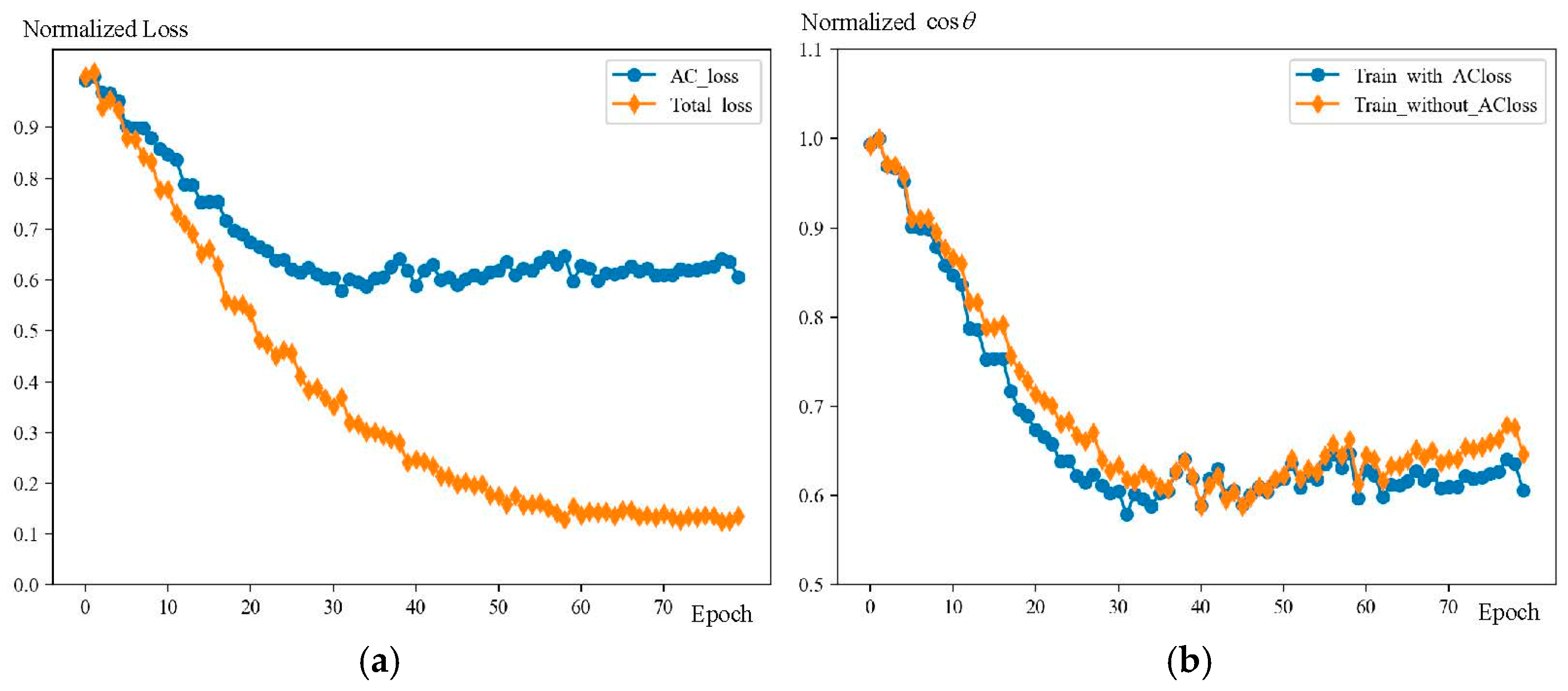
For the classifier in the network, a multi-stage regularization method is proposed to correct the recognition bias caused by catastrophic forgetting. Through analyzing the operation of the classifier, the regularization is applied to three parts involved in the classifying calculation, including the magnitude of the feature vector, the magnitude of the classifier weight vector, and the angle between them. By a staged regularization operation, the impact of catastrophic forgetting is transferred to the vector magnitude that is easier to correct. In this part, an angle constraining loss (AC loss) is introduced to constrain the angle change between new instances and old class classifier weights.
The rest of this article is organized as follows. Section 2 introduces the related work about CIL and SAR data feature fusion. The proposed SCF-CIL method is described in Section 3. Section 3 first introduces our SCF-Net, including the CNN feature extractor, SC feature extractor, and the cross-attention structure. Then, the impact of overfitting on feature space distribution is analyzed. Finally, through the derivation of the classifier operation, we proposed a multi-stage regularization method. The experimental results on the MSTAR data are analyzed in Section 4. The discussion is provided in Section 5, and the conclusions are drawn in Section 6.

2. Related Works

2.1. Class-Incremental Learning Methods

The CIL methods can be mainly divided into three parts, including replay-based methods, regularization-based methods and parameter expansion-based methods [34]. Parameter expansion-based incremental learning methods usually add extra structures to help the network to learn new knowledge, which results in a significant increase in network parameters. For the replay-based methods, they transfer the learned knowledge into instances to help the current stage of training. DGR [35] utilized the generator to offer the old data which can be input with the current data into the network for training. Iscen et al. [36] stored the feature descriptor instead of image itself to reduce the cost of memory. MER (Meta-Experience Replay) [37] combined experience replaying with meta-learning to balance between transfer and interference based on future gradients. BI-R [38] replayed with the hidden feature that is acquired by the network itself. In general, the aforementioned two methods impose higher demands on storage.
As for the regularization-based methods [39,40,41,42,43], EWC [13] used fisher information to measure the importance of the parameters and then adjusted the learning rate of the parameters accordingly. SI [44] applied intelligent synapses to the neural network to realize biological complexity, which also focused on estimating the importance of parameters. LWF [45] proposed distillation loss to balance the adjustment on the parameters of new and former classes classifiers, which focused on training data. DMC [46] first trained a model only using new instances. Then, it combined the new model and the old model with a double distillation training objective. In this way, DMC can overcome the difficulties caused by the invisible old training data.
In general, replay-based methods tend to outperform regularization-based methods because they utilize additional storage to replay or store knowledge. However, even with replay-based methods, forgetting during the CIL process is inevitable. This prompts us to consider how to more effectively minimize, rather than completely eliminate, the impact of catastrophic forgetting, for which our solution is multi-stage regularization. Initially, we guide the optimization process to allocate more of the impact caused by catastrophic forgetting onto a subset of the network parameters. Subsequently, after training, we conduct an adjustment on this subset of parameters. Through this multi-stage regularization method, we effectively mitigate the impact of catastrophic forgetting.

2.2. Electromagnetic Scattering Center Feature for SAR Target Classification

Different from the feature extracted by deep network that focuses on the image itself, the scattering center feature of radar targets contains abundant physically relevant descriptions of targets. Zhang et al. [33] proposed a feature fusion framework called FEC. It achieved effective and robust performance in SAR target classification tasks by utilizing the attributed scattering centers feature of SAR target echo data. The author transferred the scattering centers feature into a feature vector and improved the fusion effects. We are inspired that the stability and completeness of the scattering center feature could improve the performance of CIL for SAR targets. MGSFA-Net [47] obtained the multiscale global scattering features from the scattering centers of ship targets and then fused them with the deep features by weighted integration for ship target classification. EMI-Net [48] proposed an end-to-end classification network that can realize scattering centers extraction. Nowadays, the attention mechanism becomes popular in target detection and classification because of its less parameters, low module complexity, and global information processing capabilities. PAN [49] proposed a part attention network for fusing electromagnetic characteristics to classify SAR targets, which proved the effectiveness of the attention mechanism in feature fusion.
Electromagnetic scattering characteristics play a crucial role in the aforementioned methods to enhance recognition performance, demonstrating their completeness and effectiveness. This inspires us to explore how electromagnetic scattering characteristics embedded in raw radar echoes can further improve our CIL performance. Accordingly, in this paper, we employ cross-attention to integrate CNN features with scattering center features, resulting in a significant improvement in the performance of our CIL method for SAR targets.

3. Materials and Methods

In our work, the SCF-CIL is proposed for SAR targets as shown in Figure 2, which introduces three improvements on the feature extractor and the classifier aimed at overcoming catastrophic forgetting. To achieve a balance between the stability and plasticity of the extracted features, we propose a cross-attention-based feature fusion network called SCF-Net. Then, an overfitting strategy for our model is applied to reserve clustering space for future classes. To realize fair classification between the former classes and the current classes, a multi-stage regularization method is designed for the classifier. This section will provide a detailed description of our proposed improvements.

3.1. Feature Fusing Based on Cross Attention Mechanism (SCF-Net)

To utilize the inherent characteristics of SAR target data in the process of CIL, a feature fusion method based on the cross-attention mechanism is proposed, and by integrating these inherent characteristics, which are more stable compared to CNN features, a more balanced representation in terms of stability and plasticity is generated. As shown in Figure 3, for SAR targets, SAR raw data and its corresponding amplitude images are used to extract features, respectively. For the SAR amplitude image, the VGG16 network is modified to extract the CNN feature with less computation. We remove two conv 3-512 layers, one conv 3-256 layer, and all the fully connected layers. In order to apply cross attention mechanism to fusing the extracted CNN feature with electromagnetic attributed scattering center feature. The extracted CNN feature needs to be flattened to a size of 8192 × 1 . Then, through a fully connected layer, the CNN feature is converted into a size of 256 × 1 . For the SAR raw data of target, following the method in [33], we can extract the electromagnetic attributed scattering center feature (SC feature) vector, which is also with the size of 256 × 1 . First of all, N s c attributed scattering centers are estimated to obtain the parameter set. For scattering center i , its parameter set Φ i can be estimated as follows:
Φ ^ i = arg min Φ i S i A i ϕ i 2
where S is the SAR echo raw data that is transformed into a vector; A i is the complex amplitude; and ϕ i can be calculate by Equation (2) and then be transformed into a vector as well.
ϕ i f , φ = sin c 2 π L i c f sin φ φ 0 i × exp j 4 π f c x i cos φ + y i sin φ
where L i is the length of attributed scattering center i , c , f , and φ are the speed of light, frequency, and azimuth angle, respectively.
Through iterative optimization in [50], the parameter set of the scattering center i can be obtained, which contains A ^ i , L ^ i , φ ^ i , x ^ i , y ^ i , where “^” means optimized approximate results, x ^ i and y ^ i are the position coordinates of the scattering center i , respectively.
After estimating the parameters of the scattering centers, for each class that contains n samples, a parameter set with a size of n × N s c × 6 , where A ^ i is divided into A ^ i r e a l and A ^ i i m a g . A ^ i r e a l and A ^ i i m a g are the real part and the imagery part of A ^ i , respectively. With the BOVW method, the parameters set of N s c scattering centers of each target is transferred into the SC feature vector.
The lower part of Figure 3 presents a comparison between our cross-attention structure and the conventional self-attention structure. The main difference between the two attention structures lies in the way Query— Q , Key— K , and Value— V are generated. In the conventional self-attentional structure, a single feature is input and projected through three different matrices W Q , W K , and W V to obtain Q , K , and V , which are then used for feature extraction. In contrast, to achieve better feature fusion, our method takes two heterogeneous representations extracted from the SAR image and SAR echo data as Q , K , and V , respectively. This design emphasizes the interaction between the CNN-derived image features and the SC features. Specifically, the concepts of query, key, and key originate from the “query-match-retrieve” mechanism commonly used in information retrieval systems. The Query vectors are responsible for querying relevant information by matching with the Keys, while the Values provide the actual information that will be integrated into the output representation. Our SC feature is derived from the electromagnetic scattering characteristics of the target, containing rich target information, which directly reflect object-level properties. Therefore, the SC feature is particularly well-suited to serve as V . In detail, as shown in the upper part of Figure 3, CNN features f C N N are set as Q , while scattering center features f s c are set as K . The initial similarity matrix is calculated as follows:
M s = f C N N f s c T
where ( )T is the vector transposition operation. The shape of M s is 256 × 256 . Then, the primeval similarity matrix needs to be normalized.
M ˙ S = s o f t max M s d k
where d k is the dimension of k , which is also equal to the dimension of q . M ˙ s measures the importance of different semantic channel of f s c in the feature fusion process, which can be used as a weight of the feature vector. Finally, the fused feature is outputted as follows:
f = φ f c M ˙ s f s c
where the size of M ˙ s f s c is 256 × 1 . φ f c is a fully connected layer operation that transfers the size of the feature to 128 × 1 and improve the fitting ability of the network. Through this feature fusion method, the target features contained in the radar echoes are fully utilized to enhance the classification performance of our method on SAR targets, while increasing the stability of the network features to suppress the impact of catastrophic forgetting.

3.2. “Overfitting” Training Strategy for SCF-CIL

Nowadays, many mainstream incremental learning methods focus on preserving old knowledge to improve the performance. Among them, the distillation loss used in LWF is one of the most representative approaches. In addition, methods such as iCaRL, DER et al. also aim to preserve the feature representations of previous classes through different mechanisms. Similarly, our feature fusion method proposed in Section 3.1 is designed with the same goal in mind. In this section, we further conduct a theoretical analysis on how the degree of feature clustering affects the performance of incremental learning, under the assumption that the feature representations of previous classes have been sufficiently preserved. Fundamentally, classification is achieved by calculating and comparing the dot product of the feature vector with the weights of the last fully connected layer. This process determines which class the instance belongs to. For a p -class classification network, when an instance is input into the network, the classification result must fall into one of the p classes, even if the instance does not belong to any of these classes. In other words, after the normal training of the classification network, the whole feature space Θ is divided into p part Θ 1 , Θ 2 , , Θ p . After the feature extraction, the feature of the input instance must fall in one of the Θ 1 , Θ 2 , , Θ p . When CIL proceeds to the next phase, the same feature space need to be divided into p + 1 part Θ 1 , Θ 2 , , Θ p , Θ p + 1 . If applying a method that only tries to protect the former knowledge, the new features will share a part of feature space of other classes, which is one of a main reasons the accuracy of the old classes decreases in CIL process. Now that the current classes need to share a part of the feature space with the new classes, one method that could mitigate this effect is to adjust the feature clustering degree. Observing the feature clustering performance in classification network training experiments, we can conclude that a deeper network fitting degree can enhance the clustering of features in feature space. The negative impact of overfitting essentially lies in the model focusing too much on noise, fine-grained details, or spurious patterns present in the training samples. As a result, when the model encounters the samples in the validation set with different depression degrees, it becomes more susceptible to noise and sample-specific features, leading to degraded performance. In this context, the stability of extracted features—meaning their reduced sensitivity to noise and sample-specific variations during the fitting process—plays a key role in enhancing generalization. Our feature fusion method proposed in Section 3.1 improves the stability of the extracted features, thereby effectively suppressing the negative impact of slight overfitting. Therefore, this section will analyze the distribution of features and focus on modifying them to enhence the performance of the method in CIL.
Combining the conclusion about feature clustering with the description of feature space segmentation above, we can derive the schematic diagrams of feature space distribution under different conditions as shown in Figure 4a,b depict the clustering performance of features under different fitting degrees, where the scatters with different colors represent the instances from different classes. The transition from (a) to (b) illustrates the changes in feature clustering in feature space as the network fitting progresses, which can be observed during the network training process. Let us assume that the features of i -th class are distributed in the feature space with distribution g = R f , f Θ , where g is the probability of the feature falling into the position f in the whole feature space Θ . The distanse d f i between feature f and the i -th class clustering center f i , along with its variance σ i , decreases as the network fits the training data. In other words, the probability that the feature of i -th class falls at the position closer to the cluster center f i will increase. Through the above derivation, we infer the schematic diagrams of feature clustering (Figure 4c,d) in the incremental process from the observable phenomena (a) and (b). When CIL proceeds to the next stage, the distribution of the features will resemble (c) and (d). The new class ( i + 1 -th class) feature space Θ i + 1 will occupy parts of feature space of the former classes. However, the features of the former class samples will still fall into feature space Θ i + 1 with approximately the same probability as in the previous CIL stage. Therefore, the network fitting degree affects the accuracy in the incremental learning process to a certain extent. By comparing (c) and (d), the network with a higher fitting degree would achieve a higher accuracy in the next stage of incremental learning. For this reason, two overfitting strategies are applied to improve the fitting degree of the network. The first is the “late-stop” strategy, which is to train for an appropriate number of epochs after the network fitting well.
In order to alleviate the phenomenon of overfitting, it is common practice to incorporate additional structures between layers, such as dropout and batch normalization. In our CIL process, to appropriately increase the degree of network fitting, we directly connect the fully connected layers, allowing the fully connected layers before the classifier to be slightly overfitted after training. Experiments demonstrate that these two measures effectively promote the network overfitting within a safe range and improve the classification accuracy of CIL in subsequent stages without significantly reducing the accuracy in the current stage.

3.3. A Multi-Stage Regularization Method to Realize Fair Classification

In our CIL process, when training the current classes, our network does not have access to the former class instances, for which the network tends to classify former class instances as the current classes. In other words, this extreme sample imbalance leads to a significant decline in the classification performance of the CIL process.
For the last fully connected layer operation, which is also the classifier, its operation is as follows:
y = W f + b
where y is the classification result; W and b are the weight and the bias of the fully connected layer. In this paper, the bias of the classifier is ignored. (6) can also be expressed in a vector form, which makes it easier to understand the operation process of the classifier.
y k = w k f
where w k is the weight vector at k -th row of W . 1 k H represents different class within H classes. For convenience, w k is called the weight of classifier k , and y k is the output of the k-th classifier. (7) can also be written as
y k = w k f cos θ
where θ is the angle between w k and f . Now we can analyze these three elements in CIL process, separately.
In the incremental learning process, as demonstrated by previous studies on CIL, the impact of sample imbalance is almost unavoidable when there is no access to older instances. Neural network performs classification based on the learnt abstract features, with parameters optimized autonomously. In this case, in the last fully connected layer, the network will ultimately achieve preference for the current classes by simultaneously adjusting the three elements on the right side of (8). As for the feature extractor, the scattering center feature which is a manually designed feature plays an important role. It makes the extracted feature less affected by the preference of deep networks for new samples. In this case, rather than saying the old knowledge is forgotten, it is better to say that the old knowledge is “buried” by the new knowledge. Therefore, the focus of this part is how to constrain the optimization process of the classifier during the training process and how to exploit the former knowledge as much as possible after the network training.
This section adopts a strategy of constraining two of the three elements of (8) so that the impact of sample imbalance is exerted on the other one as much as possible. Then, through subsequent adjustments to this element, we can correct the bias of this element to mitigate the impact of sample imbalance after the network training.
In a large number of CIL experiments, there is a common phenomenon [51] about the distributions of w k . We make a schematic diagram to illustrate this phenomenon as shown in Figure 5.
As shown in Figure 5, when training 2 new classes, due to the sample imbalance, the l 2 n o r m of the current class weights are obviously higher than the former classes, for which the outputs of the current classes (8-th and 9-th) classifiers are much higher than others even when the input instance belongs to the old classes.
To solve this problem, feature vector normalization is introduced into the forward pass of the network, as applied to the fused feature vector f in Section 3.1, with the following formulation:
f n o r m = f f 2
to standardize the features fed into the classifier, where 2 represents l 2 n o r m . With this operation, the influence of classes imbalance on f is restrained as much as possible.
For the θ between w k and f , we find that in the classifier of the conventional recognition network, the cosine value of the angle θ between the classifier weight and the feature vector of negative sample typically remains near orthogonality. To correct the angular bias between the former classifier weight vector and the new feature vector, the cosine value is calculated as the loss function to constrain angle θ . It can be calculated as follows:
l a c = w k w k 2 f f 2
Which is our angle constraining loss (AC loss). Adding the cross-entropy loss (CE), the total loss is calculated as follows:
l = 1 λ l a c + λ l c e
where λ is a weight that needs to be assigned based on the actual situation, and l c e is the cross-entropy loss function.
l c e = 1 N k c = 1 M y i c log t i c
where M is the number of the classes. t i c is the probability that sample i is correctly classified.
y i c = 1 , l a b e l i = c 0 , l a b e l i c
where l a b e l i is the label of simple i .
It is worth noting that we do not have access to the features of old samples during training due to the limitations of the training data. As a result, our AC loss design is also constrained—currently, we can only impose angular constraints between the former classifier weights and the new sample features but not between the new classifier weights and the former sample features.
In the aforementioned regularization step, the angle θ and magnitudes of features f in Equation (8) are regularized, thereby shifting the impact of sample imbalance on the network classifier to the magnitudes of the weights w k in the CIL training process. Now we need to normalize the weights of the new classes.
w ¯ o l d = 1 N o l d 1 i N o l d i w i 2
w ¯ n e w = 1 N n e w 1 i N n e w i w i 2
where N o l d and N n e w are the number of old classes and the number of new classes, respectively. w ¯ o l d and w ¯ n e w are the averages of old classes weights and new classes weights, separately. Then, the corrected weights of new classes are calculated as follows:
w ˙ i = w ¯ o l d w ¯ n e w w i , 1 i N n e w
Through this multi-step regularization approach, we transfer and reduce the impact of sample imbalance during the CIL process, thereby enhancing the performance of CIL.

4. Results

In this section, some experiments are applied to verify the effectiveness of our improvements and the performance of our method. First, we introduce the dataset we use in the experiments. Then, a group of comparison experiments are applied to demonstrate the superiority of our method. Finally, a set of ablation experiments is conducted to validate the effectiveness of our improvements.

4.1. Experimental Dataset

The Moving and Stationary Target Acquisition and Recognition (MSTAR) dataset is used to evaluate the effectiveness of our method. In the SOCs (standard operating conditions) of MSTAR dataset, there are 10 targets collected at the depression degrees of 15 and 17 , respectively. Since classification performance on SAR target images are easily influenced by the depression angle, for a more robust validation, the dataset with 17 depression angle is used for the training, while the one with 15 is reserved for the inference phase. The specific information on the dataset we use is shown in Table 1. The SAR images and the corresponding optical images of the ten types of targets in the MSTAR dataset are shown in Figure 6.
For the CIL experiments, these 10 classes are separated into two parts: classes for basic learning and classes for incremental learning. The classes for basic learning are used to train the network to ensure it possesses sufficient feature extraction and classification capabilities. After that, the stages for incremental learning are utilized to assess the methods’ incremental learning capabilities. Considering both aspects, we select 6 classes as basic training classes and the remaining four as incremental learning classes. During each CIL stage, the network is incrementally trained with one new class, resulting in five stages, as shown in Table 1. Based on this CIL process, the comparison experiment and the ablation experiments are conducted to evaluate the effectiveness of our method.

4.2. Experimental Results

As shown in Table 2, we conducted a comparative experiment on various currently popular CIL methods, including iCaRL [19], ER [52], EWC [13], LWF [45], the Joint training method, and the None method. The Joint Training method is equivalent to training a network on all known classes, so it can be seen as the upper target of CIL. In contrast, the None method directly trains the data of the current categories in each CIL stage without taking any measures to solve catastrophic forgetting. In the new CIL stage, the None method only expands the classifier output dimension and trains the network using only the new instances. As a result, the None method at each stage can maintain only the classification ability of the current context, while the classification accuracies of former classes drop to nearly 0.2. The None method can be seen as the lower target of CIL. In addition to the above-mentioned methods, iCaRL and ER are replay methods, while EWC and LWF are regularization-based methods. Following the hyperparameters settings in some open-source implementations, the EWC regularization coefficient λ is set to 10 6 . The sample budget is set to 20 samples per old class in both ER and iCaRL. For the methods used for comparison, they are directly applied to the MSTAR dataset without any modifications. Therefore, the above methods directly extract features from the MSTAR target images for training. The five stages of the CIL experiment are conducted on these methods under the SOCs of the MSTAR dataset as used in our method. In each stage, the average accuracy a c c ¯ of all seen classes (former classes and new classes in the current stage) is reported for each algorithm in Table 2.
Since the basic learning stage does not involve the problem of catastrophic forgetting, the classification performance of these methods is not significantly different. In this stage, our method fuses richer features, leading to a slight increase in classification performance. In stage 2, the LWF method achieves the best performance, second only to joint training. However, the accuracy of LWF drops rapidly in the subsequent incremental learning stages. Its accuracy in stage 5 is only 41.645%, which is only better than the lower target. In contrast, iCaRL and ER achieve relatively stable and high performance during the incremental process. This is mainly due to the fact that these two methods have access to a part of former instances that can be used to train the network. For our method, because it does not have access to former instances, it is inevitable that its classification performance will decrease as CIL progresses. However, through our contribution, our method effectively improves the classification performance in the face of catastrophic forgetting. As shown in Table 2, our method achieves the best performance in the first 4 stages without considering the upper target. Compared with LWF, which also has no access to old instances, our method has a significantly smaller decrease in accuracy at each CIL stage.
To further compare the performance of different algorithms on new and former categories data, we separately output the accuracy of the aforementioned algorithms on both new and former categories data as shown in Figure 7a,b. Figure 7b shows that, except for our method, the new class accuracy of other methods remains at a relatively high level (within the range of 0.9 to 1) during stage 2 and stage 3, while the new class accuracy of our method drops to around 0.8. On the other hand, all other methods, except for the joint method and ours, exhibit significantly lower accuracy in the old classes. Our method trades a slight, acceptable drop in new class accuracy for a greater retention of old knowledge. However, according to Figure 7a, our method shows a significant decline at stage 5, which is caused by the combined influence of multiple factors. The most important of all, because each CIL training begins from the training result at the last CIL step, the impact bring by catastrophic forgetting accumulates over every incremental learning step, which leads to a noticeable decrease in CIL performance at stage 5. For our proposed CIL method, dataset and experiment settings in this paper, according to Table 2 and Figure 7, the proposed CIL method is effective within three incremental steps, beyond which the performance degradation becomes more noticeable.
To explore the cause of the performance decline of our method on old classes at stage 3, the t-SNE visualization results for our method and LWF at stage 3 are shown in Figure 7c,d. Our feature distributions of the former classes (classes 1–7) show more compact intra-class distributions and better inter-class separability compared to those of LWF, particularly for classes 6 and 7. In the output of LWF, class 7 exhibits more overlap with the new class, and the new class features are more tightly clustered. In contrast, our method presents a trade-off in the clustering of the new class features, which provides better preservation of former knowledge. It is worth noting that the features used for t-SNE visualization here are taken from the input to the final classifier layer. Our method further reduces the impact of the overlapping region between the new class and class 7 on the classification accuracy of class 7 by applying regularization in the final classifier, distributing the impact across both class 7 and class 8. This prevents a significant decline in the accuracy of the old classes, though it also contributes to the suboptimal classification performance observed in the newly added class. In other words, our method achieves a better balance between stability and plasticity, leading to overall superior performance in the CIL process.

5. Discussion

To verify the effectiveness of the innovations proposed in this paper, we conducted an ablation experiment, which can be divided into three parts, targeting fusing scattering center feature, our overfitting training strategy, and the proposed AC loss, respectively.

5.1. Experiments on Scattering Center Feature

The first group of experiments aims to evaluate two improvements of our SCF-Net, including fusing scattering center feature and the cross-attention mechanism. In order to compare the impact of fusing the scattering center feature on algorithm performance, we first compare the CIL performance when using only CNN feature, only SC feature, and our fused feature separately on the MSTAR dataset under SOCs. For the baseline using only the CNN feature, we adopt the VGG 16 network. For our proposed fused feature, our SCF-Net is applied. For the evaluation of only using SC feature, we simply replace the cross-attention structure in our SCF-Net with a fully connected layer to process the SC feature, while keeping the rest of the network architecture unchanged. The distillation loss is applied in the training of only using CNN feature and only using SC feature. In addition, because VGG16 is an end-to-end training network, it can be optimized using the distillation loss, which means that it follows the LWF method and can represent the performance of the LWF on our dataset. The comparison is shown in Figure 8.
Figure 8 shows the CIL results of (1) blue: only using the image feature extracted by CNN (CNN feature), (2) green: only using the SC feature, and (3) yellow: fusing the image feature and scattering center feature (SC feature). In the experiment on the CIL with only SC feature, the accuracy on training set can reach 97.28%, which means the SC feature contains enough information for classification task. However, the accuracy on validation dataset (different depression angle) is only 88.07%, which means training with only SC feature under the current network structure leads to limited generalization capability. On the other hand, while the SC feature may not achieve optimal recognition performance at the basic training stage, it exhibits a slower decline in accuracy during subsequent CIL stages compared to using only CNN feature, indicating its robustness in maintaining consistent target representations. Compared with CNN feature, it is significant that our fusing feature not only greatly improves the accuracy in the CIL process but also achieves a better classification result at the basic learning stage. In other words, using the fused features can not only effectively improve the performance of the CIL process but also achieve state-of-the-art performance in conventional classification tasks.
As discussed in Section 4.2, the impact of catastrophic accumulates over every incremental learning step. Based on the accumulated catastrophic forgetting, the method using only CNN features shows an earlier degradation than our method. The most significant disparity between the two methods in the CIL process occurs in stage 4, with our classification accuracy reaching 84.749%, while the method using VGG16 decreases to 47.282%. This is mainly because it lacks the stability and strong generalization ability provided by the SC features. By combining SC features, the fused features become more robust, making the model better able to handle the effects of accumulated forgetting across incremental stages.
The previous experiment validates the effectiveness of fusing the SC feature. Typically, when fusing multiple feature vectors, researchers often employ fully connected layer operations. To demonstrate the superiority of our cross-attention feature fusion method, we conducted comparative experiments, as illustrated in Figure 9. The blue line (Fully Connected) represents the CIL results obtained by applying the fully connected layer method for feature fusion, while the orange line (Attention) represents our cross-attention method.
In Figure 9, the disparity in CIL performance between the two methods is significantly smaller compared to the previous set of comparative experiments, providing further evidence that fused scattering center features can improve CIL performance. However, at the basic learning stage, the “Fully Connected” method achieves a classification accuracy of 95.450%, while the “CNN Feature” method achieves 98.082%. This indicates that relying solely on fully connected layers for feature fusion is not an optimal approach for integrating the two features in our study. Our cross-attention fusion method consistently outperforms the “Fully Connected” method in terms of CIL performance across all stages. In essence, our cross-attention method effectively takes advantage of the stability of the scattering center feature.

5.2. Experiments on Overfitting Mechanism

According to the derivation about late-stop and dropout, this part of the experiment mainly focuses on the impact of overfitting on feature clustering. First of all, we output the distance variance of features. For two features f i and f j both belong to one class C L A S S k , the distance between them is calculated as follows:
d i s i j k = f i f j E u c l i d e a n , i , j C L A S S k , i j
where E u c l i d e a n is the Euclidean distance. Because we pay more attention to the degree of fluctuation of feature clustering in the CIL process, we present the mean standard deviation of this distance at each training epoch as follows:
d i s a v e e = 1 N C L A S S × k N C L A S S 1 N C L A S S k i , j N C L A S S k 1 N C L A S S k N C L A S S k 1 i , j N C L A S S k d i s i , j k
where N C L A S S is the number of classes, and N C L A S S k is the number of the instances belongs to C L A S S k . Then, we obtain Figure 10, which shows the difference between d i s with and without dropout in different training stages.
Firstly, based on the two accuracy change trends (ACC with dropout and ACC without dropout) in Figure 10, the network without dropout fits faster than the network with dropout. Then, from the two standard deviation (std) trends (cluster STD with dropout and cluster STD without dropout), it is observed that the standard deviation without dropout consistently remains lower than that with dropout. This observation validates that removing the dropout structure contributes to enhancing the stability of feature clustering. Furthermore, as the accuracy increases rapidly, the standard deviation also exhibits a rapid increase. Subsequently, std will gradually decrease as training progresses, indicating that that “late-stop” can also help to increase the stability of feature clustering.
We additionally employ the T-SNE method to visualize the difference in feature distributions between the network with and without dropout at the 80th epoch with the same hyperparameters, as shown in Figure 11.
The scatter points in six colors represent features of six classes. Compared to (b), it is evident that in (a) the distance between features belonging to the same classes is smaller. This observation confirms that the features extracted by the network without dropout have a higher clustering level, which is expected to enhance the performance of CIL.
The feature extractor in our paper utilizes the scattering feature, resulting in more stable extracted features. Consequently, the optimization of the network has a greater impact on the fully connected layers after the feature extractor. Since the magnitude of the feature vector and the classifier weights in our paper are all reset to the same value, separately, the calculation of fully connected layers can be considered as the projection of the extracted feature onto the classifier weights. Therefore, we analyze the projection of features onto the classifier weight as depicted in Figure 12.
Taking class c as an example, the black arrow represents the classifier weight vector, while the blue arrows represent the feature vectors of class c. The vectors in other colors are the features of other classes. The scatter points of different colors on the black arrow represent the projections of the endpoints of different feature vectors on the weight vector. Set the direction of the black arrow as the coordinate axis, the starting point of all vectors (black point) as the origin, and the positions of the features’ projection points are the corresponding outputs of the c-th classifier. Because of the projection, the multi-label classification task becomes a binary classification task. For class c, the cluster center of positive ( m e a n c ) is calculated as follows:
m e a n c = 1 N c i = 1 N c w c f i
where N c represents the number of instances that belongs to class c. Then, the mean standard deviation of the features belonging to all different classes is calculated as follows:
s t d ¯ = 1 N C L A S S c C l a s s e s i = 1 N c w c f i m e a n c N c
Since the samples are projected on the same coordinate axis, the standard deviation can represent not only the stability of feature clustering but also the mean distance between the projected features and the clustering center, which can be used to measure the density of features clustering. The training results with and without dropout are shown in Figure 13.
The characteristics of Figure 13 resemble those of Figure 10. However, compared with Figure 10, the impact of removing dropout and “late-stop” in Figure 13 is even more evident, as the STD curves drop more significantly after around 10 epochs, and reach lower values than the STD with Dropout in the later training stages. This experiment result validates the derivation of our two methods from the perspectives of clustering stability and density.
In our specific experimental setting, the removal of dropout and the use of the “late-stop” strategy appear to improve feature clustering. Next, we conduct a CIL experiment to evaluate the effect of the overfitting strategy on CIL performance. Four methods are employed, as illustrated in Table 3, where “✔” represents the corresponding method is applied and “-” means that it is not.
As shown in Figure 14, it can be seen that both “Removing Dropout” and “Late-Stop” lead to improvements in the performance of the CIL stage to varying degrees, among which only applying “Late-Stop” has the smallest improvement. It is worth noting that the highest classification accuracy at the basic stage is achieved at 99.147% when using the initial network model. The blue line with the best performance in subsequent CIL, which applies our two methods, is 98.540% at the basic stage. In other words, our overfitting method sacrifices recognition performance to some extent at the basic stage in exchange for improvement in CIL.
Among the four models, the “Dropout and Late Stop” brings the smallest improvement. Its accuracy in the first and second stages is 88.955% and 84.920%, respectively, while the accuracy in the first and second stages of the initial method is 88.578% and 84.662%, respectively. However, the improvement brought by only removing the dropout is very obvious. In the first and second stages, the accuracy values are 93.099% and 87.827%, respectively. This phenomenon occurs because dropout slows down the network fitting process by probabilistically deactivating neurons, which is more effective than the impact of late-stop. However, comparing the gap between the blue and yellow lines with the gap between the green and red lines, it can be seen that the performance improvement brought by late stopping is different under different conditions. This is due to the randomness introduced by dropout to the training process which largely affects the learning process of the network.

5.3. Experiments on AC Loss Function

For the AC loss proposed in the paper, we conduct experiments to verify the effectiveness of the AC loss function on restricting angle during network training and the improvement of CIL performance. Firstly, Figure 15a shows the trends of the total loss and our AC loss in 80 epochs. For better visual clarity, the values of both losses were normalized. As shown in Figure 15a, both the total loss and AC loss decrease smoothly without obvious fluctuations, showing that our model achieves effective and stable fitting, and adding our AC loss will not disrupt the convergence process or compromise training stability. Then, an ablation comparison about AC loss is applied, including “only backpropagate CE loss” and “backpropagate CE loss and AC loss”. The training process of both methods adopts the same hyperparameters such as the learning rate and the optimizer. Figure 15b shows the cos θ trends of the above two methods, where θ represents the angle between the new feature and the former classifier weight as described in Section 3.3. Lower cosine values correspond to angles that are closer to being orthogonal. From Figure 15b, the model trained with AC loss exhibits a faster decrease in the cosine value ( cos θ ), indicating a quicker progression toward orthogonality between the new class features and the old-class classifier weights. More importantly, as training proceeds, the model without AC loss shows a gradual increase in cos θ , suggesting that the orthogonality is being weakened, and the new samples are increasingly interfering with the classification performance of old classes. In contrast, the model with AC loss maintains a relatively stable cos θ after convergence, demonstrating the effectiveness of the proposed constraint. This phenomenon explains why our method achieves better performance on old-class classification compared to other approaches.
Considering that the value of the loss is difficult to control in the learning process, we compare the cosine values of the angles between new class features and old classifier weights when network training reaches different accuracy rates, which is called sampling accuracies in this paper, including 0.4, 0.5, 0.6, 0.7, 0.8, 0.9, and 0.95. The experimental results are shown in Table 4. It should be noted that since the network training progress is difficult to intervene manually, it is verified in the test phase after each stage of training whether the accuracy exceeds the sampling accuracy for the first time, so as to acquire our experimental results. As shown in Figure 15b, regardless of whether our proposed AC loss is applied or not, the cos θ values exhibit unstable oscillations after 30 epochs. This instability contributes to the deviation observed at the 0.7 sampling point. We have taken measures to obtain experimental data that best meets the requirements. However, for the sampling accuracy of 0.7, the accuracies of the two networks are quite different which are 0.704 and 0.749, respectively. From Table 4, it can be concluded that when the network trained with AC loss reaches a certain accuracy, the angle between the new feature vector and old classifier weight is smaller than the network trained without AC loss, indicating that it is closer to orthogonality. This proves that our AC loss has a certain constraint effect on the angle during the network optimization process.
Since our AC loss applies angular constraints only between the new feature vectors and the former classifier weights, we also conducted an experiment to analyze the effect of our AC loss on the angle between the former classifier weight vector and the former feature vector. The angular changes in training process are output as shown in Figure 16: (a) angular changes between old-class sample features and their corresponding classifier weight vectors during training. (b) Angular changes between old-class sample features and non-corresponding classifier weight vectors (i.e., weights of other classes) during training. The blue line represents training without AC loss; the orange line represents training with AC loss in both (a) and (b). Since the AC loss imposes constraints on both the former classifier weights and the feature of new classes in learning process, it slightly affects the angle between the old class features and old classifier weights. However, as shown in Figure 17, the overall training performance under the CIL setting benefits from the introduction of the AC loss, leading to a slight improvement.
The effect of AC loss on CIL is also compared experimentally, as shown in Figure 17. As can be seen from the figure, the network trained with AC loss is slightly better than the network without AC loss at all stages of the CIL process. The largest difference is in stage 5, where the two accuracies are 57.019% and 65.151%, respectively, with a difference of 8.13%. This part of the experiment proves that AC loss can improve the performance of CIL.

6. Conclusions

In this paper, we propose a class-incremental learning method called SCF-CIL. By incorporating a cross-attention mechanism, our SCF-Net effectively leverages the electromagnetic information contained in SAR data, while combining the stability of SC features with the plasticity of CNN features, improving the performance of CIL methods on SAR data. A comparison experiment shows that fusing the SC feature with cross-attention greatly improves the CIL performance on SAR targets. Afterward, the effect of network overfitting on the feature space is analyzed, and two training strategies, “removing dropout” and “late-stop”, are introduced to improve feature clustering degree, thereby reserving feature space for subsequent incremental learning in our specific model setting. Four groups of experiments are conducted to demonstrate the impact of overfitting on feature clustering and the improvements in CIL performance due to slight overfitting. Since the SC feature is manually extracted, and in order to further correct the former class recognition bias caused by sample imbalance, a multi-stage regularization method is proposed. Through regularization at different stages, it transfers the impact of catastrophic forgetting to vector modules that are easier to process. In this part, this paper proposes an AC loss, which constrains the angle between the new feature vector and the old classifier weight in the CIL training process. Our experiment also proves the effectiveness of the AC loss. In addition to that, we compare our SCF-CIL with six commonly used CIL methods. Our method achieves the optimal CIL performance in the five stages of the CIL process. In summary, the SCF-CIL method has good effectiveness and robustness in SAR targets CIL process and great potential in the application of an SAR recognition system.
Our experiments show the effectiveness of utilizing the information contained in SAR images and demonstrate that there is still room for improvement in the performance of CIL methods on SAR targets. However, the extraction and integration of SAR image information in our current work remain insufficient. In the future, we will focus on an end-to-end incremental learning network and improve our feature fusion method to enhance the intelligence of radar systems.

Author Contributions

The contribution of authors is stated as follows: methodology and formulation, Y.Z. and J.Z.; software realization, Y.Z.; validation and experiments, Y.Z.; writing and review, Y.Z., J.Z. and S.V.; funding acquisition, M.X. and J.Z. All authors have read and agreed to the published version of the manuscript.

Funding

This work was supported in part by the Key Program of the National Natural Science Foundation of China under Grant 62331020, the National Natural Science Foundation of China under Grant 62301403, and China Scholarship Council program (Project ID: 202306960013).

Data Availability Statement

The raw data supporting the conclusions of this article will be made available by the authors on request.

Conflicts of Interest

The authors declare no conflicts of interest.

References

  1. Xu, G.; Zhang, B.; Yu, H.; Chen, J.; Xing, M.; Hong, W. Sparse Synthetic Aperture Radar Imaging from Compressed Sensing and Machine Learning: Theories, applications, and trends. IEEE Geosci. Remote Sens. Mag. 2022, 10, 32–69. [Google Scholar] [CrossRef]
  2. Ni, P.; Xu, G.; Zhong, Z.; Chen, J.; Hong, W. SAR Target Recognition Using Complex Manifold Multiscale Feature Fusion Network. In Proceedings of the IGARSS 2024—2024 IEEE International Geoscience and Remote Sensing Symposium, Athens, Greece, 7–12 July 2024; pp. 3532–3535. [Google Scholar]
  3. Huang, Y.; Wang, D.; Wu, B.; An, D. NST-YOLO11: ViT Merged Model with Neuron Attention for Arbitrary-Oriented Ship Detection in SAR Images. Remote Sens. 2024, 16, 4760. [Google Scholar] [CrossRef]
  4. Li, S.; Yang, X.; Lv, X.; Li, J. SAR-MINF: A Novel SAR Image Descriptor and Matching Method for Large-Scale Multidegree Overlapping Tie Point Automatic Extraction. Remote Sens. 2024, 16, 4696. [Google Scholar] [CrossRef]
  5. Feng, S.; Fu, X.; Feng, Y.; Lv, X. Single-Scene SAR Image Data Augmentation Based on SBR and GAN for Target Recognition. Remote Sens. 2024, 16, 4427. [Google Scholar] [CrossRef]
  6. Li, G.; Liu, W.; Gao, Q.; Wang, Q.; Han, J.; Gao, X. Self-Supervised Edge Perceptual Learning Framework for High-Resolution Remote Sensing Images Classification. IEEE Trans. Circuits Syst. Video Technol. 2024, 34, 6024–6038. [Google Scholar] [CrossRef]
  7. Ai, J.; Mao, Y.; Luo, Q.; Jia, L.; Xing, M. SAR Target Classification Using the Multikernel-Size Feature Fusion-Based Convolutional Neural Network. IEEE Trans. Geosci. Remote Sens. 2022, 60, 1–13. [Google Scholar] [CrossRef]
  8. Oh, J.; Youm, G.Y.; Kim, M. SPAM-Net: A CNN-based SAR target recognition network with pose angle marginalization learning. IEEE Trans. Circuits Syst. Video Technol. 2021, 31, 701–714. [Google Scholar] [CrossRef]
  9. Geng, J.; Ma, W.; Jiang, W. Causal Intervention and Parameter-Free Reasoning for Few-Shot SAR Target Recognition. IEEE Trans. Circuits Syst. Video Technol. 2024, 34, 12702–12714. [Google Scholar] [CrossRef]
  10. Wang, R.; Su, T.; Xu, D.; Chen, J.; Liang, Y. MIGA-Net: Multi-view Image Information Learning Based on Graph Attention Network for SAR Target Recognition. IEEE Trans. Circuits Syst. Video Technol. 2024, 34, 10779–10792. [Google Scholar] [CrossRef]
  11. Wu, J.; Fang, L.; Yue, J. TAKD: Target-Aware Knowledge Distillation for Remote Sensing Scene Classification. IEEE Trans. Circuits Syst. Video Technol. 2024, 34, 8188–8200. [Google Scholar] [CrossRef]
  12. Goodfellow, I.J.; Mirza, M.; Xiao, D.; Courville, A.; Bengio, Y. An empirical investigation of catastrophic forgetting in gradient-based neural networks. arXiv 2014, arXiv:1312.6211. [Google Scholar]
  13. Kirkpatrick, J.; Pascanu, R.; Rabinowitz, N.; Veness, J.; Desjardins, G.; Rusu, A.A.; Milan, K.; Quan, J.; Ramalho, T.; Grabska-Barwinska, A.; et al. Overcoming catastrophic forgetting in neural networks. Proc. Nat. Acad. Sci. USA 2017, 114, 3521–3526. [Google Scholar] [CrossRef] [PubMed]
  14. McCloskey, M.; Cohen, N.J. Catastrophic interference in connectionist networks: The sequential learning problem. Psychol. Learn. Motiv. 1989, 24, 109–165. [Google Scholar]
  15. Thrun, S. Is learning the n-th thing any easier than learning the first? Proc. Adv. Neural Inf. Process. Syst. 1996, 8, 640–646. [Google Scholar]
  16. Li, Z.; Jin, K.; Xu, B.; Zhou, W.; Yang, J. An improved attributed scattering model optimized by incremental sparse Bayesian learning. IEEE Trans. Geosci. Remote Sens. 2016, 54, 2973–2987. [Google Scholar] [CrossRef]
  17. Fan, J.; Wang, X.; Wang, X.; Zhao, J.; Liu, X. Incremental Wishart broad learning system for fast polsar image classification. IEEE Geosci. Remote Sens. Lett. 2019, 16, 1854–1858. [Google Scholar] [CrossRef]
  18. Dang, S.; Cao, Z.; Cui, Z.; Pi, Y.; Liu, N. Open set incremental learning for automatic target recognition. IEEE Trans. Geosci. Remote Sens. 2019, 57, 4445–4456. [Google Scholar] [CrossRef]
  19. Rebuffi, S.-A.; Kolesnikov, A.; Sperl, G.; Lampert, C.H. ICaRL: Incremental classifier and representation learning. In Proceedings of the 2017 IEEE Conference on Computer Vision and Pattern Recognition (CVPR), Honolulu, HI, USA, 21–26 July 2017; pp. 2001–2010. [Google Scholar]
  20. Lopez-Paz, D.; Ranzato, M. Gradient episodic memory for continual learning. Proc. Adv. Neural Inf. Process. Syst. 2017, 30, 6467–6476. [Google Scholar]
  21. Mallya, A.; Lazebnik, S. PackNet: Adding multiple tasks to a single network by iterative pruning. In Proceedings of the 2018 IEEE/CVF Conference on Computer Vision and Pattern Recognition (CVPR), Salt Lake City, UT, USA, 18–23 June 2018; pp. 7765–7773. [Google Scholar]
  22. Serra, J.; Suris, D.; Miron, M.; Karatzoglou, A. Overcoming catastrophic forgetting with hard attention to the task. In Proceedings of the 35th International Conference on Machine Learning, Stockholm, Sweden, 10–15 July 2018; Volume 80, pp. 4548–4557. [Google Scholar]
  23. Tang, J.; Xiang, D.; Zhang, F.; Ma, F.; Zhou, Y.; Li, H. Incremental SAR automatic target recognition with error correction and high plasticity. IEEE J. Sel. Topics Appl. Earth Observ. Remote Sens. 2022, 15, 1327–1339. [Google Scholar] [CrossRef]
  24. Ammour, N.; Bazi, Y.; Alhichri, H.; Alajlan, N. Continual learning approach for remote sensing scene classification. IEEE Geosci. Remote Sens. Lett. 2022, 19, 1–5. [Google Scholar] [CrossRef]
  25. Li, Y.; Wu, W.; Luo, X.; Zheng, M.; Zhang, Y.; Peng, B. A Survey: Navigating the Landscape of Incremental Learning Techniques and Trends. In Proceedings of the 2023 18th International Conference on Intelligent Systems and Knowledge Engineering (ISKE), Fuzhou, China, 17–19 November 2023; pp. 163–169. [Google Scholar]
  26. Park, J.-I.; Park, S.-H.; Kim, K.-T. New discrimination features for SAR automatic target recognition. IEEE Geosci. Remote Sens. Lett. 2013, 10, 476–480. [Google Scholar] [CrossRef]
  27. Clemente, C.; Pallotta, L.; Gaglione, D.; De Maio, A.; Soraghan, J.J. Automatic target recognition of military vehicles with Krawtchouk moments. IEEE Trans. Aerosp. Electron. Syst. 2017, 53, 493–500. [Google Scholar] [CrossRef]
  28. Kang, M.; Ji, K.; Leng, X.; Xing, X.; Zou, H. Synthetic aperture radar target recognition with feature fusion based on a stacked autoencoder. Sensors 2017, 17, 192. [Google Scholar] [CrossRef]
  29. Ding, B.; Wen, G.; Ma, C.; Yang, X. An efficient and robust framework for SAR target recognition by hierarchically fusing global and local features. IEEE Trans. Image Process. 2018, 27, 5983–5995. [Google Scholar] [CrossRef] [PubMed]
  30. Simonyan, K.; Zisserman, A. Very deep convolutional networks for large-scale image recognition. arXiv 2014, arXiv:1409.1556. [Google Scholar]
  31. Filliat, D. A visual bag of words method for interactive qualitative localization and mapping. In Proceedings of the 2007 IEEE International Conference on Robotics and Automation, Rome, Italy, 10–14 April 2007; pp. 3921–3926. [Google Scholar]
  32. Zhang, Y.; Jin, R.; Zhou, Z.-H. Understanding bag-of-words model: A statistical framework. Int. J. Mach. Learn. Cybern. 2010, 1, 43–52. [Google Scholar] [CrossRef]
  33. Zhang, J.; Xing, M.; Xie, Y. FEC: A feature fusion framework for SAR target recognition based on electromagnetic scattering features and deep CNN features. IEEE Trans. Geosci. Remote Sens. 2021, 59, 2174–2187. [Google Scholar] [CrossRef]
  34. Lu, X.; Sun, X.; Diao, W.; Feng, Y.; Wang, P.; Fu, K. LIL: Lightweight incremental learning approach through feature transfer for remote sensing image scene classification. IEEE Trans. Geosci. Remote Sens. 2022, 60, 1–20. [Google Scholar] [CrossRef]
  35. Shin, H.; Lee, J.K.; Kim, J.; Kim, J. Continual learning with deep generative replay. Proc. Adv. Neural Inf. Process. Syst. 2017, 30, 2990–2999. [Google Scholar]
  36. Iscen, A.; Zhang, J.; Lazebnik, S.; Schmid, C. Memory-efficient incremental learning through feature adaptation. arXiv 2020, arXiv:2004.00713. [Google Scholar]
  37. Riemer, M.; Cases, I.; Ajemian, R.; Liu, M.; Rish, I.; Tu, Y.; Tesauro, G. Learning to learn without forgetting by maximizing transfer and minimizing interference. arXiv 2018, arXiv:1810.11910. [Google Scholar]
  38. van de Ven, G.M.; Siegelmann, H.T.; Tolias, A.S. Brain-inspired replay for continual learning with artificial neural networks. Nat. Commun. 2020, 11, 4069. [Google Scholar] [CrossRef] [PubMed]
  39. Hou, S.; Pan, X.; Loy, C.C.; Wang, Z.; Lin, D. Lifelong learning via progressive distillation and retrospection. In Proceedings of the European Conference on Computer Vision (ECCV), Munich, Germany, 8–14 September 2018; pp. 437–452. [Google Scholar]
  40. Castro, F.M.; Marín-Jiménez, M.J.; Guil, N.; Schmid, C.; Alahari, K. End-to-end incremental learning. In Proceedings of the European Conference on Computer Vision (ECCV), Munich, Germany, 8–14 September 2018; pp. 233–248. [Google Scholar]
  41. Dhar, P.; Singh, R.V.; Peng, K.-C.; Wu, Z.; Chellappa, R. Learning without memorizing. In Proceedings of the 2019 IEEE/CVF Conference on Computer Vision and Pattern Recognition (CVPR), Long Beach, CA, USA, 15–20 June 2019; pp. 5138–5146. [Google Scholar]
  42. Liu, X.; Masana, M.; Herranz, L.; Van de Weijer, J.; Lopez, A.M.; Bagdanov, A.D. Rotate your networks: Better weight consolidation and less catastrophic forgetting. In Proceedings of the 2018 24th International Conference on Pattern Recognition (ICPR), Beijing, China, 20–24 August 2018; pp. 2262–2268. [Google Scholar]
  43. Cermelli, F.; Mancini, M.; Bulo, S.R.; Ricci, E.; Caputo, B. Modeling the background for incremental learning in semantic segmentation. In Proceedings of the IEEE/CVF Conference on Computer Vision and Pattern Recognition (CVPR), Seattle, WA, USA, 13–19 June 2020; pp. 9233–9242. [Google Scholar]
  44. Zenke, F.; Poole, B.; Ganguli, S. Continual learning through synaptic intelligence. Proc. Mach. Learn. Res. 2017, 70, 3987. [Google Scholar] [PubMed]
  45. Li, Z.; Hoiem, D. Learning without forgetting. IEEE Trans. Pattern Anal. Mach. Intell. 2018, 40, 2935–2947. [Google Scholar] [CrossRef]
  46. Zhang, J.; Zhang, J.; Ghosh, S.; Li, D.; Tasci, S.; Heck, L.; Zhang, H.; Kuo, C.C.J. Class-incremental learning via deep model consolidation. In Proceedings of the IEEE/CVF Winter Conference on Applications of Computer Vision (WACV), Snowmass Village, CO, USA, 1–5 March 2020; pp. 1120–1129. [Google Scholar]
  47. Zhang, X.; Feng, S.; Zhao, C.; Sun, Z.; Zhang, S.; Ji, K. MGSFA-Net: Multi-scale global scattering feature association network for SAR ship target recognition. IEEE J. Sel. Topics Appl. Earth Observ. Remote Sens. 2024, 17, 4611–4625. [Google Scholar] [CrossRef]
  48. Liao, L.; Du, L.; Chen, J.; Cao, Z.; Zhou, K. EMI-Net: An End-to-End Mechanism-Driven Interpretable Network for SAR Target Recognition Under EOCs. IEEE Trans. Geosci. Remote Sens. 2024, 62, 1–18. [Google Scholar] [CrossRef]
  49. Feng, S.; Ji, K.; Wang, F.; Zhang, L.; Ma, X.; Kuang, G. PAN—Part attention network integrating electromagnetic characteristics for interpretable SAR vehicle target recognition. IEEE Trans. Geosci. Remote Sens. 2023, 61, 1–17. [Google Scholar] [CrossRef]
  50. Duan, J.; Zhang, L.; Xing, M.; Liang, Y. Novel feature extraction method for synthetic aperture radar targets. J. Xidian Univ. (Natural Sci.) 2014, 41, 13–19. [Google Scholar]
  51. Liu, M.; Huang, L. Teamwork is not always good: An empirical study of classifier drift in class-incremental information extraction. arXiv 2023, arXiv:2305.16559. [Google Scholar]
  52. Rolnick, D.; Ahuja, A.; Schwarz, J.; Lillicrap, T.; Wayne, G. Experience replay for continual learning. Proc. Int. Conf. Neural Inf. Process. Syst. 2019, 32, 350–360. [Google Scholar]
Figure 1. The overall illustration of the class-incremental learning (CIL) process, where new classes (red arrow) are introduced stage by stage, and the model incrementally learns to classify all seen classes.
Remotesensing 17 01586 g001
Figure 2. Overview of the SCF-CIL framework, including a cross-attention feature fusion module (SCF-Net), an overfitting training strategy for the feature extractor, and a multi-stage regularization method for the classifier. The feature extractor produces SC features and CNN features, which are fused through a cross-attention mechanism and further refined by multiple fully connected layers, serving as the input to the final classifier.
Remotesensing 17 01586 g002
Figure 3. Structure of our SCF-Net.
Remotesensing 17 01586 g003
Figure 4. Schematic diagram of feature space distribution in CIL process: (a,b) demonstrate the changes in feature clustering observed during the network fitting process, while (c,d) are the schematic diagrams of the changes in feature clustering during CIL process obtained by our derivation.
Remotesensing 17 01586 g004
Figure 5. Histogram of classifier output. (a) Training 7 classes simultaneously. (b) Incrementally training 2 classes after training 6 classes.
Remotesensing 17 01586 g005
Figure 6. Instances of 10 target classes in the MSTAR dataset. (SAR images and their corresponding optical image).
Remotesensing 17 01586 g006
Figure 7. Comparison of algorithms on accuracy for former and new classes. (a) Comparison of algorithms on accuracy for former classes. (b) Comparison of algorithms on accuracy for new classes. (c) T-SNE visualization result of our method. (d) T-SNE visualization result of LWF.
Remotesensing 17 01586 g007
Figure 8. Experiment results for different features.
Remotesensing 17 01586 g008
Figure 9. Comparison of different feature fusing methods.
Remotesensing 17 01586 g009
Figure 10. Mean variance of feature clustering distance in feature space.
Remotesensing 17 01586 g010
Figure 11. Feature distribution of different network structures.
Remotesensing 17 01586 g011
Figure 12. Schematic diagram of the projection of features onto the classifier weight vector. (a) Projection diagram of positive and negative features. (b) Projection diagram of multiple classes features on one certain classifier weight vector.
Remotesensing 17 01586 g012
Figure 13. Mean variance of feature clustering distance in feature projection space.
Remotesensing 17 01586 g013
Figure 14. Ablation experiments on “Removing dropout” and “Late-stop”.
Remotesensing 17 01586 g014
Figure 15. Effectiveness analysis of the proposed AC loss on training performance. (a) Normalized total loss and AC loss during training. (b) Evolution of the normalized cosine distance ( cos θ ) between old class weights and new sample features, with and without the proposed AC loss.
Remotesensing 17 01586 g015
Figure 16. Angular changes in training process. (a) Angular changes between old-class sample features and their corresponding classifier weight vectors during training. (b) Angular changes between old-class sample features and non-corresponding classifier weight vectors (i.e., weights of other classes) during training.
Remotesensing 17 01586 g016
Figure 17. Experiment on our AC loss.
Remotesensing 17 01586 g017
Table 1. Data distribution of MSTAR SOCs.
Class NameSerialTraining Set
( 17 )
Testing Set
( 15 )
CIL
Stages
ZSU_23_4d08299274stage 5
ZIL131E12299274stage 4
T72132232196stage 3
T62A51299273stage 2
D713015299274Basic Learning
(stage 1)
BTR70c71233196
BTR607532256195
BRDM2E-71298274
BMP29563233195
2S1B01299274
Table 2. Comparison of experiment results of different CIL methods on the MSTAR dataset (average accuracy %). Italic font indicates the upper and lower bounds for reference, and bold font highlights the best CIL performance in each CIL stage.
Basic LearningStage 2Stage 3Stage 4Stage 5
None98.08252.89343.46934.42030.861
Joint training98.08296.37795.76197.82996.284
ICaRL [19]97.99579.53663.80165.27260.000
ER [52]98.08276.63471.93277.99763.719
LWF [45]98.08296.25264.93347.28241.645
EWC [13]98.08280.04371.97067.32146.267
Ours98.54095.98490.49584.74967.044
Table 3. Four methods in the ablation experiment.
LineBlueOrange Green Red
Removing dropout--
“Late-stop”--
Table 4. Ablation experiment on our AC loss.
0.40.50.60.70.80.90.95
CEloss0.210.180.160.140.160.130.11
ACloss + CEloss0.160.140.140.150.150.120.09
Disclaimer/Publisher’s Note: The statements, opinions and data contained in all publications are solely those of the individual author(s) and contributor(s) and not of MDPI and/or the editor(s). MDPI and/or the editor(s) disclaim responsibility for any injury to people or property resulting from any ideas, methods, instructions or products referred to in the content.

