A Subimage Autofocus Bistatic Ground Cartesian Back-Projection Algorithm for Passive Bistatic SAR Based on GEO Satellites

Abstract

As an evolutionary advancement to conventional synthetic aperture radar (SAR), passive bistatic SAR (PBSAR) utilizing geostationary orbit (GEO) satellite signals demonstrates significant potential for high-resolution imaging. However, PBSAR faces dual challenges in computational efficiency and phase error compensation. Traditional accelerated back-projection (BP) variants developed from monostatic SAR are incompatible with PBSAR’s geometry, and autofocus BP (AFBP) methods exhibit prohibitive computational costs and inadequate space-variant phase error handling. This study first develops a bistatic ground Cartesian back-projection (BGCBP) algorithm through subimage wavenumber spectrum correction, specifically adapted to GEO-satellite-based PBSAR. Compared to conventional BP, the BGCBP achieves an order-of-magnitude complexity reduction without resolution degradation. Building upon this foundation, we propose a subimage autofocus BGCBP (SIAF-BGCBP) methodology, synergistically integrating autofocus processing with BGCBP’s accelerated framework. SIAF-BGCBP reduces phase estimation’s complexity by 90% through subimage pixel density optimization while maintaining estimation accuracy. Further enhancement of SIAF-BGCBP via geometric inversion would enable the precise compensation of space-variant phase errors while remaining efficient. Simulations and real-environment experiments verify the effectiveness of the proposed methods.

1. Introduction

Passive bistatic synthetic aperture radar (PBSAR) has garnered significant interest from researchers due to its flexibility, high resolution, and concealment capabilities [1,2,3]. However, PBSAR still faces substantial challenges in developing fast imaging and autofocus (AF) algorithms [4]. This paper focuses on accelerating the imaging algorithm and autofocus processing for PBSAR based on geostationary orbit (GEO) satellites.

Given the complex configuration of PBSAR, traditional frequency-domain algorithms, such as the range Doppler algorithm, frequency scaling algorithm, and range migration algorithm, are difficult to apply directly [5,6]. The back-projection (BP) algorithm is a time-domain approach, which performs pixel-by-pixel imaging, and BP is adaptable to any configuration and imaging plane, making it suitable for PBSAR [7,8]. However, its high computational complexity necessitates the exploration of an accelerated BP algorithm [8,9].

Several accelerated BP algorithms have been developed by dividing multiple sub-apertures (SAs), including fast BP (FBP), fast factorized BP (FFBP), accelerated fast BP (AF-BP), Cartesian factorized BP (CFBP), etc. [10]. FBP and FFBP produce local rough imaging results using local polar coordinates (LPCs) and achieve high-resolution images through interpolation [11,12]. Additionally, some FBP variants employ locally mixed LPCs to simplify the interpolation process [13]. AF-BP utilizes global polar coordinates for imaging, eliminating the need for two-dimensional interpolation compared to FFBP [14]. However, due to imaging condition constraints, the wavenumber spectrum of subimages must be unambiguous in AF-BP, increasing the computational demands during the image fusion [15]. Unlike accelerated BP algorithms based on polar coordinates, accelerated BP algorithms using Cartesian coordinate (CC) decomposition have gained increasing attention [16,17,18,19,20]. Compared to LPC-based accelerated BP algorithms, CFBP eliminates the need for interpolation, enhancing imaging quality and efficiency [21]. However, the radar trajectory in CFBP is relatively simple, and CFBP can only image the range-azimuth plane in a small range of the frontal side view, an approach that may not meet the requirements for SAR imaging in complex maneuvering scenarios [22]. Most importantly, the above methods are difficult to apply to PBSAR because of straight-trajectory assumptions and idealized imaging planes (trajectory-normal side configurations).

To address these limitations, ground Cartesian BP (GCBP) is designed for SAR imaging with flexible maneuvering trajectories and imaging planes, offering higher computational efficiency and accuracy without pointwise interpolation operations [20,22]. However, GCBP is derived from monostatic SAR configurations and requires correction of the wavenumber support region based on the phase history before subimage fusion, preventing its direct application to PBSAR [20]. In this paper, we extend GCBP to GEO-satellite-based PBSAR and propose bistatic GCBP (BGCBP). By analyzing the wavenumber spectrum in PBSAR, we compensate for and correct the bistatic phase interference term, enabling fast imaging in PBSAR.

Building upon the computational efficiency advantages of the BGCBP framework in PBSAR implementations, this study further introduces a synergistic integration framework that systematically combines the BGCBP with an AF back-projection (AFBP) algorithm, achieving optimization of phase error compensation accuracy and processing efficiency.

The parametric AF algorithm has been gradually abandoned due to its lack of accuracy, particularly in addressing high-order phase errors [23]. Map drift requires enhanced hardware and still faces challenges with high-order phase errors [24]. Non-parametric autofocus algorithms primarily fall into two categories: phase gradient autofocus (PGA) and image quality metric (IQM)-based AFBP algorithms [25,26,27,28]. Traditional PGA relies on the key assumption that the Fourier transform (FT) relationship exists between the image domain and the range-compressed phase domain [29]; however, this relationship does not hold in BP images. While accelerated BP based on mixed LPCs can approximate the FT relationship, it is only applicable to monostatic SAR with straight trajectories [13].

The IQM-based AFBP is adaptable to the BP algorithm, making it flexible and universal [28]. Key IQMs include image entropy, contrast, and sharpness [30,31,32]. Notably, the sharpness-based AFBP stands out because it offers a closed-form solution for optimal phase estimation through mathematical extrapolation, eliminating the need for iterative optimization required by other IQMs [33,34,35,36].

However, AFBP methodologies suffer from computational complexity that hinders their real-time implementation, as they are performed as a post-processing of BP images [37]. Additionally, traditional AFBP methodologies demonstrate deficiencies in addressing spatial variations in phase error due to their reliance on simplified signal models [33]. This paper proposes the subimage autofocus BGCBP (SIAF-BGCBP) algorithm for GEO-satellite-based PBSAR, integrating the sharpness-based AFBP with the BGCBP algorithm. We introduce two AF strategies tailored to different scenarios.

For cases where the spatial variability in the phase error is negligible, we combine the SIAF with BGCBP to perform AF processing in the subimage (SI) domain. The deep integration of the AF algorithm with BGCBP accelerates the entire signal processing flow and enhances parallelism.

For scenarios where the spatial variability in the phase error is significant, such as in large imaging scenes, we propose a phase retrieval technique based on SI segmentation and geometric inversion (GI). By optimizing multiple local SIs, the true antenna position is determined and applied to image refocusing.

In summary, the main contributions of this paper are as follows:

• For the GEO-satellite-based PBSAR, we analyze the wavenumber spectrum and enhance the traditional GCBP to develop BGCBP, extending its applicability to PBSAR.
• To address the limitations of traditional AF algorithms, we integrate the image-sharpness-based SIAF with the proposed BGCBP, improving efficiency and parallelism.
• We propose distinct AF strategies for different scenarios, enhancing the focusing accuracy while maintaining the processing speed.

The proposed methodology resolves the tradeoff between autofocus precision and computational complexity in PBSAR implementations, as quantitatively validated through simulations and real-environment experiments.

The remainder of this paper is structured as follows: Section 2.1 presents the signal model; Section 2.2 provides the wavenumber spectrum analysis of PBSAR and details the derivation of the BGCBP algorithm; Section 2.3 analyzes the characteristics of the phase error, presents the proposed SIAF-BGCBP algorithm, and outlines the autofocus strategies for two different cases; Section 3 discusses the simulations and real-environment experiments; and Section 4 offers a conclusion and future prospects.

2. Materials and Methods

2.1. Model

The geometric configuration of the GEO-satellite-based PBSAR studied in this paper is shown in Figure 1. The satellite operates in GEO, with the reference antenna stationary and its beam directed at the satellite. Meanwhile, the receiving antenna is mounted on a mobile platform, such as a vehicle or aircraft, creating a synthetic aperture to achieve high azimuth resolution.

2.1.1. Signal Model

Suppose that the signal emitted by the radiation source at the slow time $t_m$ is $p(t,t_m)$, where $t$ represents the fast time. The echo of the scattering center $P_i$ can be expressed as shown in Equation (1):

$$s\left(t,t_m;P_i\right)=p(t-\tau (t_m;P_i),t_m)\exp \left(-j2\pi f_c(t-\tau (t_m;P_i))\right)$$

(1)

where $f_c$ represents the carrier frequency, $P_i=(x_i,y_i,z_i)$ represents the coordinates of the scattering center, and $\tau$ represents the bistatic time delay of the $P_i$ relative to the reference signal. Equation (2) gives the exact expression of $\tau$, where $c$ is the speed of light, $R_{bi}$ is the bistatic distance delay, and $R_{ref}$, $R_t$, and $R_r$ are the reference path, incident path, and reflected path, respectively:

$$\left\{\begin{array}{l}\tau (t_m;P_i)=R_{bi}(t_m;P_i)/c\\ R_{bi}(t_m;P_i)=R_t(t_m;P_i)+R_r(t_m;P_i)-R_{ref}(t_m)\end{array}\right.$$

(2)

The assumption that the reference antenna and the echo antenna in the PBSAR are located on the same platform is adopted in Equation (2), aligning with the typical PBSAR configuration. To maintain unity with the PBSAR involved in this paper, a local coordinate system was established with the stationary reference antenna as the origin, as shown in Figure 1. The detailed coordinates for the reference antenna, the radiation source, and the echo antenna are $P_{ref}=(0,0,0)$, $P_t=(P_{t,x},P_{t,y},P_{t,z})$, and $P_r(t_m)=(P_{r,x}(t_m),P_{r,y}(t_m),P_{r,z}(t_m))$, respectively. Thus, specific expressions of $R_{ref}$, $R_t$, and $R_r$ can be further arranged, as shown in Equation (3):

$$\begin{array}{ccc}{R}_t(P_i)={‖P_t-P_i‖}_2& R_r(t_m;P_i)={‖P_r(t_m)-P_i‖}_2& R_{ref}={‖P_t-P_{ref}‖}_2\end{array}$$

(3)

The echo after the range compression can be written as shown in Equation (4), where $\sigma (P_i)$ and $B$ denote the reflectance of $P_i$ and the signal bandwidth, respectively:

$$s_{rc}\left(t,t_m;P_i\right)=\sigma (P_i)\mathrm{sinc}\left(\left[t-\tau (t_m;P_i)\right]/B\right)\exp \left(-j2\pi f_c\tau (t_m;P_i)\right)$$

(4)

Given the predominance of systemic measurement error effects on echo phase perturbations, we adopted the standard practice of excluding amplitude variations [38]. This phase-centric assumption permits derivation of the range-compressed signal spectrum, as shown in Equation (5):

$$s_{rc}\left(f_r,t_m;P_i\right)=\mathrm{rect}\left({\displaystyle \frac{f_r}{B}}\right)\exp \left(-j2\pi \left(f_r+f_c\right)R_{bi}\left(t_m;P_i\right)/c\right)$$

(5)

Define $\phi \left(t_m;P_i\right)=-2\pi \left(f_r+f_c\right)R_{bi}\left(t_m;P_i\right)/c$ as representing the phase history, which is determined by the bistatic distance delay $R_{bi}\left(t_m;P_i\right)$.

With the satellite and the reference antenna statically positioned, positioning errors can be treated as constant throughout the experiment, making the motion error primarily a result of the echo antenna’s non-ideal movement [32,39]. Suppose that the trajectory deviation $e(t_m)$ of the echo antenna is expressed as shown in Equation (6). Then, $R_r$ can be reformulated as shown in Equation (7):

$$e(t_m)=\left[\begin{array}{c}\Delta x(t_m),\Delta y(t_m),\Delta z(t_m)\end{array}\right]$$

(6)

$$R_r(t_m;P_i)={‖P_r(t_m)+e(t_m)-P_i‖}_2$$

(7)

Then, the expression of bistatic slant distance can also be reformulated as shown in Equation (8), where $R_{bi,id}(t_m;P_i)$ represents the ideal bistatic slant distance, while $\Delta R$ and $\Delta R_{t,ref}$ denote the bistatic slant range error caused by echo antenna trajectory deviations and positioning errors of the radiation source and reference antenna, respectively:

$$\begin{array}{ll}{R}_{bi}(t_m;P_i)& =R_t(P_i)+R_r(t_m;P_i)-R_{ref}\\ & =R_{bi,id}(t_m;P_i)+\Delta R(t_m;P_i)+\Delta R_{t,ref}\end{array}$$

(8)

At this stage, the signal model for GEO-satellite-based PBSAR is fully established, incorporating the effect of motion error. Notably, the motion trajectory of the echo antenna is not predefined during the modeling process, making the model applicable to PBSAR systems with arbitrary trajectories.

2.1.2. Analysis of the Signal Model

Equation (5) highlights that GEO-satellite-based PBSAR differs from conventional monostatic SAR; it employs a separate transceiver configuration, with the reference antenna and echo antenna also separated, forming the unique characteristics of the PBSAR studied in this paper. The phase history of the target echo is influenced by the incident, reflected, and reference paths, necessitating the development of an imaging algorithm that is tailored to these system characteristics. Additionally, Equations (5) and (8) illustrate the effects of phase errors, considering spatial variability.

The PBSAR system loses the azimuth invariance due to platform separation. The acceleration variants of BP are generally derived based on the monostatic and straight-trajectory assumptions, so the adaptability is limited [12]. In contrast, GCBP is based on curvilinear trajectories, making it promising for application to the PBSAR, so we explored BGCBP algorithms suitable for PBSAR based on GCBP.

The BGCBP algorithm is well suited for the PBSAR, and IQM-based AFBP algorithms exhibit inherent synergies with the BGCBP framework.

$$\begin{array}{ll}{R}_{bi}(t_m;P_i)& =R_t(P_i)+R_r(t_m;P_i)-R_{ref}\\ & =R_{bi,id}(t_m;P_i)+\Delta R(t_m)+\Delta R_{t,ref}\end{array}$$

(9)

The bistatic slant range error $\Delta R$ in Equation (8) depends on both the slow time and the scattering center, making it both time- and space-varying. Nevertheless, estimating and compensating for phase errors separately for each scattering center is impractical. Traditional AFBP algorithms simplify this by assuming no spatial variability in phase errors, allowing Equation (8) to be reduced to Equation (9). However, this assumption is only valid for original or small-area imaging. When these conditions are not met, the spatial variability in the phase errors significantly affects the accuracy of phase estimation, leading to the failure of traditional AFBP algorithms.

Therefore, it is essential to develop an AFBP algorithm that accounts for the spatial variation in phase error and that can be integrated with BGCBP to achieve high efficiency and accuracy.

2.2. Bistatic Ground Cartesian Back-Projection Algorithm

To solve the limitation of the application of the traditional accelerated BP algorithms in PBSAR, the traditional GCBP is first introduced in this section, followed by the development of the proposed BGCBP.

2.2.1. The Derivation of the Original GCBP

Partitioning SAs is a consistent practice to accelerate BP, and GCBP follows the same idea. In conventional monostatic SAR, the echo phase and slant range model for a scattering center $P=\left(x_0,y_0,0\right)$ can be expressed as shown in Equation (10). This constitutes the configuration differences and fundamental distinction between monostatic SAR and PBSAR.

$$\begin{array}{l}\phi \left(t_m,x_0,y_0\right)=\exp \left(-j{K}_{r}R\left(t_m,x_0,y_0\right)\right)\\ R\left(t_m,x_0,y_0\right)=2\left(\begin{array}{l}\sqrt{{(P_{r,x}(t_m)-x_0)}^2+{\left(P_{r,y}(t_m)-y_0\right)}^2+H^2}\\ +\Delta r(t_m,x_0,y_0)\end{array}\right)\end{array}$$

(10)

Define $K_r=4\pi (f_c+f_r)/c$, denoting the wavenumber in the range direction. $\overrightarrow{R}$ is the range vector pointing toward the target $P$ from the ideal antenna phase center (APC) of the echo antenna, and ${\overrightarrow{K}}_r$ is the wavenumber vector along the direction of $\overrightarrow{R}$. Equation (11) provides the wavenumber-domain expression of the echo signal:

$$S_{rc}(K_r,t_m)=\exp \left(-j\left(\overrightarrow{R}+\overrightarrow{e}\left(t_m\right)\right)\cdot {\overrightarrow{K}}_r\right)$$

(11)

The subimage $I_n(x,y)$ of the $n\mathrm{th}$ SA is expressed as shown in Equation (12), where $K_{rc}$ represents the range wavenumber corresponding to the center frequency, which is generally the carrier frequency, $f_c$:

$$I_n(x,y)={\displaystyle \underset{t_{m,n}}{\int }{\displaystyle {\int }_{K_{rc}-\frac{2\pi B}{c}}^{K_{rc}+\frac{2\pi B}{c}}{S}_{rc}\left(K_r,t_m\right)\exp \left(j{\overrightarrow{K}}_r\overrightarrow{R}\right)d{K}_{r}d{t}_m}}$$

(12)

The wavenumber domain of $I_n(x,y)$ is given by Equation (13), where $F_x$ and $F_y$ represent the azimuth and range frequencies of the SI, respectively; $t_{m,n}$ denotes the slow-time duration of the $n\mathrm{th}$ SA; and $W_r$ and $W_a$ represent the range and azimuth scope of the partial imaging grid, respectively:

$$I_n(F_x,F_y)={\displaystyle {\int }_{-W_r/2}^{W_r/2}{\displaystyle {\int }_{-W_a/2}^{W_a/2}{I}_i}}(x,y)\exp (-j{F}_{x}x)\times \exp (-j{F}_{y}y)dxdy$$

(13)

Decompose the wavenumber vector ${\overrightarrow{K}}_r$ into ${\overrightarrow{K}}_x$, ${\overrightarrow{K}}_y$, and ${\overrightarrow{K}}_z$, corresponding to the azimuth wavenumber vectors along the x-axis, y-axis, and z-axis in Figure 1, respectively. The spectrum $I\left(K_x,K_y\right)$ of the SI is analyzed from the wavenumber perspective.

During the integration process in Equation (13), the principle of stationary phase (POSP) is applied multiple times, with the constant phase term and the amplitude omitted [20,22]. The final integration result is as presented in Equation (14). The trajectory deviation exists in a phase form in the frequency domain, without affecting the calculation of the frequency spectrum [20].

$$I\left(K_x,K_y\right)=\exp (-j{K}_{x}x-j{K}_{y}y-j\Delta \phi (K_x,K_y))$$

(14)

$\Delta \phi (K_x,K_y)$, in Equation (14), is the phase error of the SI in the wavenumber spectrum domain, resulting from the motion error $\Delta r(t_m,x_0,y_0)$. Referring to Equation (14), the wavenumber spectrum support region of the target is linearly related to the target’s position but is independent of the radar’s position [20]. When trajectory errors are disregarded, the two-dimensional inverse Fourier transform of Equation (14) produces a well-focused image.

In the GCBP, the 2D spectrum of the SI comprises only the linear term related to the position and the phase error term. Additionally, the spectral range of the imaging result matches the wavenumber range produced during imaging; thus, the GCBP algorithm is a wavenumber spectrum recovery algorithm. Since the derivation process does not require a predefined trajectory for the moving platform or a specific aperture length, GCBP is versatile and capable of adapting to more complex SAR configurations.

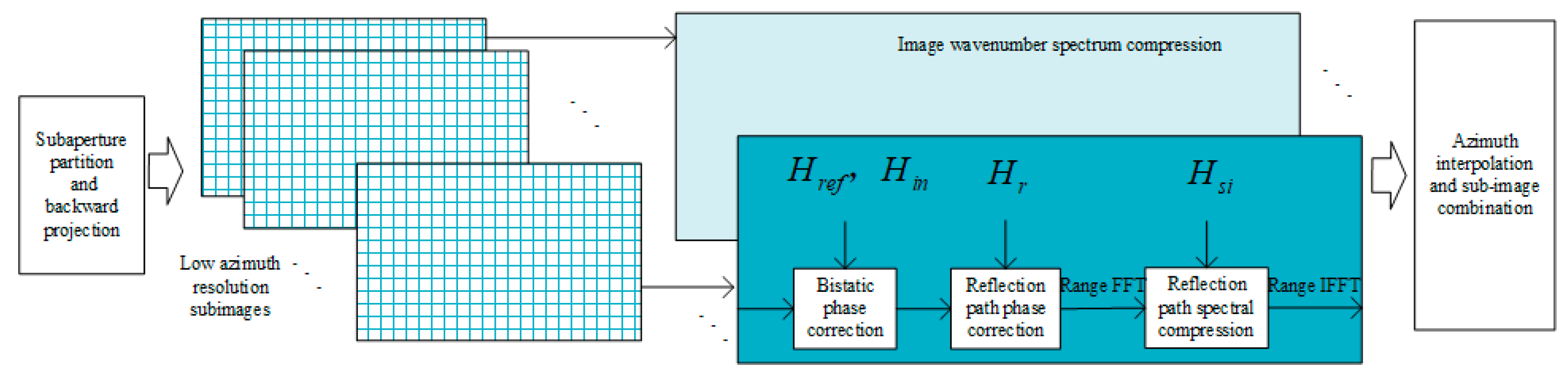
2.2.2. BGCBP for PBSAR Based on the GEO Satellite

While GCBP offers adaptability to complex motion trajectories, its application in PBSAR systems still presents certain challenges. The primary challenge arises from the alteration of the slant range model in the PBSAR, as highlighted by the comparison between Equations (8) and (10). For the convenience of analysis, the effect of trajectory error is not considered for the time being.

The derivation of Equation (13) refers to the POSP, which is difficult to apply due to the relatively complex configuration of PBSAR [15]. When the slant range model aligns with Equation (8), the phase of the integral in Equation (13) for PBSAR is as given in Equation (15). As with the monostatic SAR in the previous section, the height of $P_i$ is ignored in the analysis, which is common practice in SAR analysis [20], as SAR has a high two-dimensional resolution, and BP can be easily combined with a digital elevation map to eliminate the influence of height [33].

$$K_{\mathrm{r}}{R}_{bi}(t_m,P_i)-F_{x}x-F_{y}y$$

(15)

In PBSAR, $K_{\mathrm{r}}$, in Equation (15), is redefined as $K_r=2\pi (f_c+f_r)/c$. The acquisition of Equation (16) is obtained with the derivative of Equation (15) with respect to $x$ equal to zero, according to the POSP; $x_s$ denotes the static phase point:

$$F_x=K_{\mathrm{r}}\left({\displaystyle \frac{P_r(t_m)-x_s}{R_r(t_m;x_s,y)}}+{\displaystyle \frac{P_{t,x}-x_s}{R_t(x_s,y)}}\right)$$

(16)

The influence of the three paths makes the stationary phase difficult to solve.

$$\begin{array}{l}\sqrt{\begin{array}{l}{K_r}^2-{F_x}^2+\\ {\displaystyle \frac{{K_r}^2{(P_{t,x}-x)}^2}{R_t^2}}-{\displaystyle \frac{2F_x{K}_r{(P_{t,x}-x)}^2}{R_t}}\end{array}}\cdot \sqrt{{(P_{r,y}(t_m)-y)}^2+P_{r,z}^2(t_m)}\\ +{\displaystyle \frac{K_r}{R_t}}{(P_{t,y}-y)}^2+{P_{t,z}}^2-{\displaystyle \frac{K_r(P_t-x)(P_{r,x}(t_m)-P_{t,x})}{R_t}}-F_x{P}_{r,x}(t_m)-F_{y}y\end{array}$$

(17)

There are multiple perturbation terms in the wavenumber spectrum of the SI in (17) due to the multiple-square-root form of the phase of the PBSAR [40,41]. The stationary phase is difficult to solve, and the wavenumber spectrum cannot be expressed directly in mathematical form. When $P_t$ equals $P_r$, the PBSAR simplifies to a monostatic SAR, and Equation (17) can be further reduced and expressed as Equation (18):

$$\sqrt{K_{\mathrm{r}}^2-F_x^2}\sqrt{{\left(P_{r,y}\left(t_m\right)-y\right)}^2+P_{r,z}{\left(t_m\right)}^2}-F_x{P}_{r,x}\left(t_m\right)-F_{y}y.$$

(18)

In PBSAR, the bistatic disturbance term causes a shift and distortion in the spectral support region. As a result, significant spectral errors in the bistatic case can lead to severe fusion errors, hindering subsequent processing. The bistatic perturbation term is crucial for ensuring successful combination.

PBSAR based on GEO satellites is characterized by the fact that the GEO satellite and reference antenna remain relatively geostationary while the echo antenna moves. Therefore, the reference path remains constant throughout the imaging process, the incident path is space-varying but time-invariant, and the echo path varies in both space and time with space–time coupling. Therefore, the reference path will cause the overall offset of the wavenumber support region, while the incident path will cause the space-varying misalignment of the wavenumber support region [20].

The reference path, being constant and time-invariant, has a minimal impact on the integral and can be easily compensated. The phase compensation function for the spectral error caused by the reference path can be expressed as shown in Equation (19):

$$H_{ref}=K_{rc}\sqrt{{(P_{t,x}-P_{r,x})}^2+{(P_{t,y}-P_{r,y})}^2+{(P_{t,z}-P_{r,z})}^2}$$

(19)

Comparing different phase histories, the incident path is a key factor in causing bistatic disturbances. To obtain an accurate wavenumber spectrum, proper alignment compensation is necessary. Given its spatial variation with time-invariance, compensating within the SI domain is an effective approach. The phase compensation function for the incident path can be expressed as shown in Equation (20):

$$H_{in}(x,y)=-K_{rc}\sqrt{{(P_{t,x}-x)}^2+{(P_{t,y}-y)}^2+{(P_{t,z}-z)}^2}$$

(20)

Then, Equation (15) can be reformulated as follows:

$$K_{\mathrm{r}}\sqrt{{(P_{r,x}(t_m)-x)}^2+{(P_{r,y}(t_m)-y)}^2+{(P_{r,z}(t_m))}^2}-F_{x}x-F_{y}y$$

(21)

Based on the POSP, the derivative of Equation (21) with respect to $x$ is zero, meaning that the stationary phase point $x_s$ satisfies Equation (22):

$$\begin{array}{l}{F}_x=-K_r{\displaystyle \frac{P_{r,x}-x}{R_r(t_m,x,y)}}\\ F_y=-K_{\mathrm{r}}{\displaystyle \frac{P_{r,y}(t_m)-y}{R_r(t_m;x,y)}}\end{array}$$

(22)

Substituting Equation (22) into Equation (21) yields the result shown in Equation (18). Similarly, applying the POSP to Equation (18), the final expression of the integral is as shown in Equation (23):

$$I_n(F_x,F_y)=\exp (-j{F}_{x}x-j{F}_{y}y)$$

(23)

Including the effect of trajectory bias, Equation (23) will yield the same result as Equation (14). At this stage, the wavenumber-domain analysis of the SI in GEO-satellite-based PBSAR is performed. By correcting the deviation in the wavenumber support region based on the geometric configuration, the accurate wavenumber support region of the SI is obtained which depends solely on the spatial position of the scattering center.

2.2.3. Analysis of Spectral Compression

To effectively enhance the resolution of SA images through coherent synthesis, the image must meet the target spectrum’s sampling requirements; otherwise, an insufficient sampling rate will cause blurring. Traditional FBP and FFBP algorithms exploit the low sampling rate needed for the angular dimension, so the sampling rate can be significantly reduced without causing spectrum aliasing in LPCs.

The yield requirements for both distance and angle dimensions in LPCs are generally described by Equation (24) [10,11]:

$$\begin{array}{cc}\Delta r\le {\displaystyle \frac{c}{2B\cos (\beta /2)}}& \Delta (\cos \theta )\le {\displaystyle \frac{c}{2l{f}_{\min }}}\end{array}$$

(24)

where $f_{\min }$ denotes the minimum frequency corresponding to the minimum wavenumber $K_{r,\min }$ of the spectral support region. The 2D support regions of the wavenumber spectrum are described in Equation (25), where ${\theta }_{\max }$ and ${\theta }_{\min }$ are the maximum and minimum values of the slant angle, respectively [21].

$$\left\{\begin{array}{c}K\sin {\theta }_{\min }\le K_x\le K\sin {\theta }_{\max }\\ K_{\min }\cos \theta \le K_y\le K_{\max }\cos \theta \end{array}\right.$$

(25)

The requirement for imaging grid sampling for SAs based on CC is as shown in Equation (26), according to the Nyquist sampling theorem and the influence of bistatic configuration:

$$\begin{array}{cc}\Delta x\le {\displaystyle \frac{2\pi }{K({\theta }_{\max }-{\theta }_{\min })}}& \Delta y\le {\displaystyle \frac{2\pi }{B\cos (\beta /2)}}\end{array}$$

(26)

In PBSAR, the squint angle is primarily influenced by the angle between the receiving antenna and the scene, as well as the antenna’s beam angle. Consequently, a high sampling rate is essential for image quality. However, the low pixel capacity at low sampling rates is crucial for accelerating BP through SA division. Therefore, before performing coherent accumulation between subimages, the beam spectrum support region of the subimages must be compressed and corrected.

The influence of the reference and incident paths is compensated by $H_{ref}$ and $H_{in}\left(x_i,y_i\right)$. The effect of the reflected path on the wavenumber spectrum will be corrected immediately afterwards. The spectral center of the target is defined by the central moment of the SA because of the short duration. The spatial location of the scattering center and the varying inclination of the wavenumber support region’s centerline influence the expansion of this support region. The wavenumber expression of the target point can be written as shown in Equation (27):

$$\begin{array}{cc}{K}_{xc}{|}_{x_i,y_i}={\displaystyle \frac{P_{r,x}(t_m)-x_i}{R_r(t_m;x_i,y_i)}}{K}_{rc}& K_{yc}{|}_{x_0,y_0}={\displaystyle \frac{P_{r,y}(t_m)-y_i}{R_r(t_m;x_i,y_i)}}{K}_{rc}\end{array}$$

(27)

The effect of the spatial location of scattering centers on the wavenumber support region can be compensated by the phase compensation function $H_r\left(x_i,y_i\right)$ in the SI domain:

$$H_r\left(x_i,y_i\right)=-K_{rc}\sqrt{{(P_{r,x}(t_m)-x_i)}^2+{(P_{r,y}(t_m)-y_i)}^2+P_{r,z}{(t_m)}^2}$$

(28)

After the compensation of Equation (28), the target’s wavenumber spectrum shifts to the center, effectively compressing the spectrum of the scattering centers. However, the PBSAR configuration causes the equivalent phase center and beam direction to change nonlinearly during imaging. Compensating the target’s spectrum from multiple angles is essential to accommodate the space-variant spectrum inclination, as shown in Figure 2.

The range block ignores the variation in the azimuth spectrum’s spread with $y$, so the center $y_c$ of the coordinate range will be used for the compensation. The phase compensation function for spectral inclination is provided by Equation (29) [22]:

$$H_{si}\left(x;K_y^{\prime }\right)=-{\displaystyle \frac{(K_y-K_{yc})}{2}}{\displaystyle \frac{{\left(P_{r,x}(t_m)-x\right)}^2}{P_{r,y}(t_m)-y_c}}$$

(29)

After four steps of spectral correction and compression, the Cartesian coordinate system’s sampling rate meets the requirements, resolving the spectral aliasing issue in subimage coherent fusion, as shown in Figure 2. Subsequent subimage accumulation can then be performed directly through zero expansion for azimuth upsampling. The direct accumulation method is more efficient and accurate, as it avoids the high computational burden and cumulative errors associated with point-by-point interpolation. Figure 3 shows the schematic flow of spectral compression.

At this stage, the complete BGCBP method is derived as an extension of GCBP; it involves four steps of spectrum compression and correction to accurately determine the wavenumber support region.

2.2.4. Analysis and Discussion of BGCBP

BGCBP utilizing SA division strategies fundamentally reduces computational complexity by decreasing the imaging grid density of SIs. Extending beyond the comprehensive mathematical derivation of BGCBP established in prior sections, this section conducts a systematic performance evaluation of the algorithm, rigorously examines its operational constraints under various imaging scenarios, and quantitatively assesses its computational efficiency improvements.

First, unlike approaches employing other coordinate systems (e.g., LPCs or hybrid coordinate systems), the BGCBP framework based on the ground Cartesian coordinate system maintains adaptable imaging plane selection. During coherent integration of multiple SIs, the Cartesian coordinates’ inherent advantages enable upsampling operations to replace the complex interpolation routines required in other coordinate systems. This dual advantage not only reduces computational overheads, but also minimizes cumulative error propagation. Consequently, in terms of imaging performance, BGCBP theoretically both preserves the operational flexibility in imaging plane determination and achieves high precision levels.

Second, this study extends the GCBP framework by leveraging the temporal decoupling between reference and incident paths in GEO-satellite-based PBSAR systems, thereby establishing the complete theoretical foundation of BGCBP. The application of BGCBP to bistatic SAR configurations with general dual-motion patterns will be systematically investigated in subsequent research. Consequently, BGCBP demonstrates enhanced operational adaptability for single stationary-transmitter/receiver bistatic SAR systems.

Finally, BGCBP is well suited for PBSAR and significantly enhances operational efficiency; this section examines its computational complexity. Key parameters for the computational complexity analysis of the algorithms are shown in

Table 1. Parameter information in the computation analysis of BGCBP.

Parameters Symbols	Meaning
$N_r$	The number of grids in the range direction for the final image
$N_a$	The number of grids in the azimuth direction for the final image
$N_{tf}$	The number of sampling points in the fast-time dimension
$N_{ts}$	The number of sampling points in the slow-time dimension
$N_{sub\_a}$	The number of sub-apertures
$N_{tfu}$	Upsampling coefficients in the fast-time dimension

.

Based on the parameters in Table 1, the basic complex multiplication operation complexity $C_{m,b}$, including range compression and upsampling, can be expressed as shown in Equation (30):

$$C_{m,b}=\left(N_{tf}\log (N_{tf})/2+N_{tf}\right)N_{ts}+\left(N_{tf}{N}_{tfu}\log (N_{tf}{N}_{tfu})/2\right)N_{ts}$$

(30)

The computational complexity in the back-projection stage is primarily influenced by the number of grids and SAs, as shown in Equation (31):

$$\left\{\begin{array}{cc}\hfill C_{m,BGCBP}\hfill & =N_r{N}_a/N_{sub\_a}{N}_{ts}+4N_r{N}_a/N_{sub\_a}\hfill \\ & +N_r{N}_{a}2+\left(N_r\log (N_r)/2\right)(N_a/N_{sub\_a}+2N_r)\hfill \\ & +\log (N_a/N_{sub\_a})N_a/N_{sub\_a}/2\hfill \\ \hfill C_{m,BP}\hfill & =N_r{N}_a{N}_{ts}\hfill \end{array}\right.$$

(31)

In summary, this section introduces BGCBP, an accelerated BP algorithm for GEO-satellite-based PBSAR. BGCBP is an extension of the GCBP algorithm for monostatic SAR, modified and enhanced to suit the PBSAR system in this paper, broadening its applicability. Compared to the traditional BP algorithm, BGCBP significantly reduces computational complexity. Significantly, the proposed BGCBP algorithm establishes a theoretical framework for integrating conventional AFBP methodologies, enabling subsequent computational acceleration of autofocus operations.

2.3. Proposed Fast Autofocus Back-Projection Algorithm

The BGCBP algorithm analysis does not account for the impact of motion errors on the imaging results. In practice, however, non-ideal platform motion significantly degrades image quality, particularly for high-frequency and large-bandwidth cases. The AFBP algorithm, as a sophisticated extension of conventional BP methodologies, inherits the inherent flexibility of BP techniques and demonstrates exceptional robustness against random high-order phase errors; however, it shares the high computational burden that is characteristic of traditional BP approaches. This inherent limitation critically impedes its practical deployment in SAR systems requiring real-time processing capabilities.

Building upon BGCBP, we propose a novel SIAF-BGCBP methodology incorporating a subimage autofocus mechanism. Prior to detailing our innovative approach, we first present conventional AFBP algorithms, establishing essential mathematical foundations for the subsequent analysis of two distinct autofocus strategies within the BGCBP method.

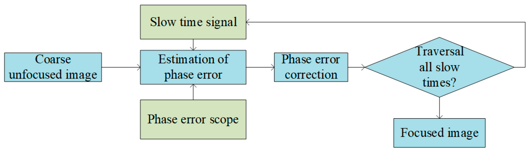
2.3.1. Conventional AFBP Algorithm Based on Sharpness

The processing flow of the traditional AFBP algorithms based on IQMs is shown in Figure 4. The IQM-based AFBP begins with the phase-corrupted, unfocused SAR image and subtracts the $m\mathrm{th}$ back-projected signal. The $m\mathrm{th}$ phase error is estimated by the IQMs. The phase of the $m\mathrm{th}$ slow-time signal is corrected and coherently added to the image. The process iterates over all slow-time signals to estimate phase errors for each, following a coordinate descent approach. If necessary, multiple iterations are performed to correct the dependencies between phase errors until a specified indicator reaches a preset threshold [37].

Based on the IQM, the phase error corresponding to the $m\mathrm{th}$ slow time can be obtained by solving the optimization problem shown in Equation (32), where $Iq$ represents the IQM, ${\varphi }_m$ is the phase compensation coefficient for the $m\mathrm{th}$ slow-time signal, and ${\widehat{\varphi }}_m$ is the optimal estimate:

$${\widehat{\varphi }}_m=\arg {\max }_{{\varphi }_m}Iq({\varphi }_m)$$

(32)

Ash introduced an AFBP method based on image sharpness [33]. Using image sharpness as the IQM, Equation (32) can be further expressed as Equation (33):

$${\widehat{\varphi }}_m=\arg {\max }_{{\varphi }_m}{\displaystyle \sum _{x,y}{I}_{m;x,y}({\varphi }_m)I_{m;x,y}^{*} ({\varphi }_m)}=\arg {\max }_{{\varphi }_m}{\displaystyle \sum _{x,y}{‖I_{m;x,y}‖}^2}$$

(33)

where $I_{m;x,y}$ denotes the complex value of the image at $(x,y,0)$, with the influence of the $m\mathrm{th}$ slow time removed. According to the mathematical deduction and geometric interpretation in [33], the optimal estimation of the phase can be obtained by solving a quartic polynomial.

As a non-parametric method, AFBP has better estimation performance. The integration of AFBP and BGCBP provides a precondition for fast autofocus processing. Thus, a combined AF based on SIs with the BGCBP algorithm is recommended in this paper.

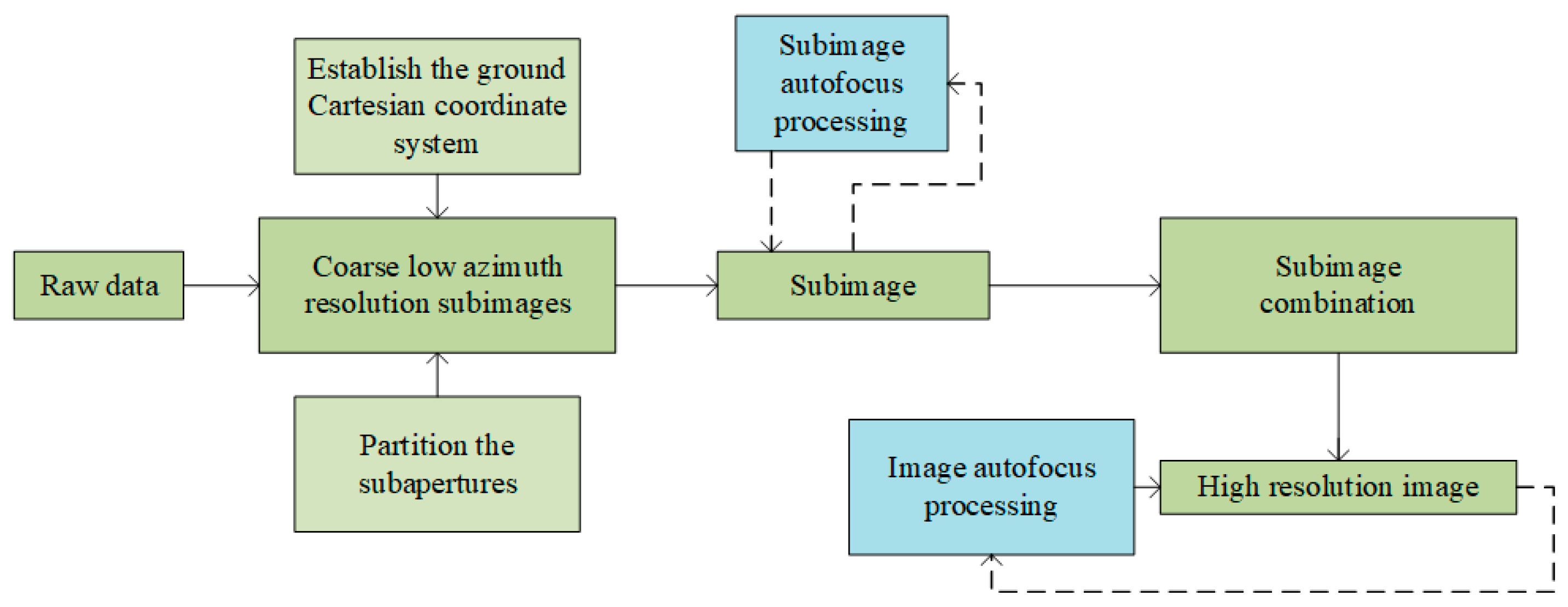
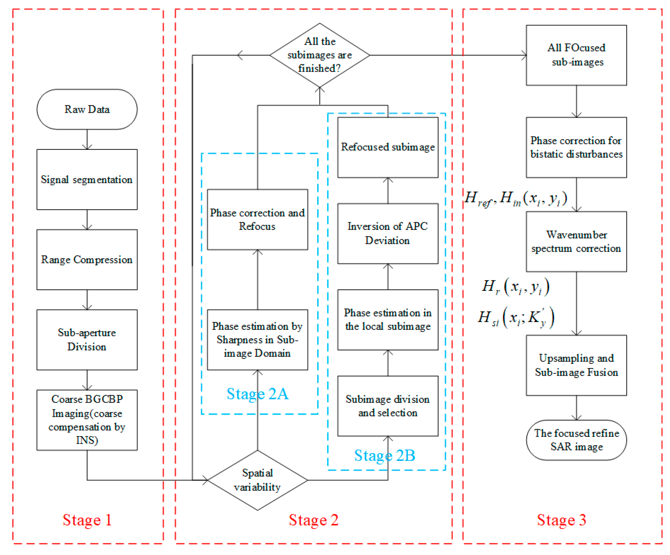
2.3.2. Subimage Autofocus Bistatic Ground Cartesian Back-Projection Algorithm

AFBP based on sharpness offers an effective estimation performance and avoids iterative processing; however, the downside of AFBP’s speed and performance is the need for matrix inversion during its solution process. Matrix inversion can be computationally expensive, especially for large matrices. The size of the matrix in AFBP is dependent on the number of pixels in the rough image. In this case, a smaller pixel capacity means less computational complexity.

In the BGCBP algorithm, SA partitioning generates SIs for coherent fusion. The reduction in the pixel capacity of the SIs significantly lowers the algorithm’s complexity, and this lower pixel count also aids in AF processing. For BGCBP, correcting the wavenumber spectrum before subimage fusion is essential, as phase errors caused by slant range inaccuracies influence the position and shape of the wavenumber spectrum’s support region. Thus, estimating phase errors in the subimage domain is a more logical approach. Therefore, this paper further enhances the algorithm by proposing SIAF-BGCBP, which achieves improved operational efficiency. The schematic diagram of the proposed method is shown in Figure 5. SIAF-BCGBP performs the AF processing in the SI stage, unlike the traditional AFBP, which performs the AF after obtaining the high-resolution image.

Based on this strategy, Equation (33) can be reformulated as Equation (34), where $I_{m,n;x,y}$ denotes the complex amplitude in the $n\mathrm{th}$ SI with the $m\mathrm{th}$ slow-time signal removed:

$${\widehat{\varphi }}_m=\arg {\max }_{{\varphi }_m}{\displaystyle \sum _{x,y}{I}_{m,n;x,y}({\varphi }_m)I_{m;x,y}^{*}({\varphi }_m)}=\arg {\max }_{{\varphi }_m}{\displaystyle \sum _{x,y}{‖I_{m,n;x,y}‖}^2}$$

(34)

AFBP is applied to each SI to determine the optimal phase error based on image sharpness. Although there are $N$ SIs that require autofocusing, the number of processing steps for each SI is reduced by a factor of $N$, keeping the total number of computations constant. The computational burden of the SIAF processing is greatly reduced due to the reduction in pixel capacity. Additionally, because the SIs are relatively independent before fusion, SIAF-BGCBP offers the potential for parallelization.

SIAF-BGCBP addresses the shortcomings in terms of efficiency; however, the AFBP algorithms based on IQMs assume that the phase error is consistent across all pixels, meaning that it does not vary spatially, as shown in Equation (9).

A simulation experiment was conducted to determine the spatial variability in the phase error; the results are shown in Figure 6. In the simulation, random motion errors, not exceeding 0.1 m, were introduced to the echo antenna. Figure 6 demonstrates that the phase error caused by these motion errors exhibits significant spatial variability. Additionally, the vertical height (z-axis) trajectory error has a minimal impact on the phase error deformation.

To address this issue, this paper explores a phase error compensation method that accounts for spatial variability, building on the SIAF-BGCBP approach. After obtaining the phase estimate ${\widehat{\phi }}_m$ of the unwinding, there is a direct correspondence between the phase error and the actual slant range $R_{m,e}$, as shown in Equation (35), enabling accurate retrieval of the APC [42,43]:

$$R_{m,e}=R_{bi,id}(t_m;P_i)+\Delta R(t_m)+\Delta R_{t,ref}=R_{bi,id}(t_m;P_i)+{\displaystyle \frac{{\widehat{\phi }}_m}{2\pi f_c}}$$

(35)

For a given SI, only one conclusion about phase error can be obtained, as solving the phase error in three-dimensional space remains challenging. Splitting one SI into multiple smaller segments generates several estimates of the slant range, effectively creating a system of quadratic equations for determining the antenna phase center. The problem is over-constraint when the number of segmented images is large enough. The system of equations can be expressed as shown in Equation (36), where the corner scale $p$ denotes the different local SIs:

$$R_{m,e,p}={‖P_{r,m}+e_{r,m}-P_p‖}_2-{‖P_{r,m}-P_p‖}_2+\Delta R_{t,ref}$$

(36)

Four local image regions are theoretically sufficient to estimate the actual antenna position. The geometric essence of solving a system of equations is to find the intersection of several ellipsoidal surfaces, potentially leading to a multi-solution problem; therefore, at least one additional local subimage region is needed to verify the accuracy of the solution. Furthermore, the GI estimation overcomes the limitations of phase space variation, allowing it to adapt to more complex bistatic imaging systems.

2.3.3. Analysis and Discussion of the Proposed SIAF-BGCBP

The two proposed SIAF strategies enable the concurrent optimization of computational efficiency and imaging fidelity through their integration with the BGCBP framework.

This paper addresses limitations of AFBP through the development of SIAF-BGCBP, which synergistically integrates autofocus capabilities with accelerated BGCBP processing architectures. Since the estimation process of the phase error does not make other adjustments, the estimation accuracy remains the same as that of the conventional AFBP.

Furthermore, AFBP’s operational paradigm incorporates critical assumptions: system errors exclusively manifest as phase distortions in the azimuth dimension, and phase errors exhibit spatial invariance [33,44]. This study retains the fundamental azimuth error assumption of traditional AFBP. The proposed SIAF-BGCBP framework achieves enhanced spatial error adaptability via GI-based refinement, enabling precise compensation of spatially variant phase errors.

When spatial variability in phase error is not the primary concern, the AF method presented in this paper is applied at the SI stage. This approach offers significant advantages, as the number of subimage pixels is much smaller than the total number of pixels in the original BP algorithm. The extent of pixel reduction depends on the number of SAs, as shown in Equation (37), where $N_{p,si}$, $N_{p,bp}$, and $N_{sa}$ denote the number of pixels in the subimage, the number of pixels in the traditional BP image, and the number of SAs, respectively. Reducing the pixel count accelerates the image sharpness calculations and decreases the computational complexity of the matrix inversion involved in the phase estimation process. Meanwhile, less computation also means less storage.

$$N_{p,si}=N_{p,bp}/N_{sa}$$

(37)

When the spatial variability in phase error significantly impacts the autofocusing algorithm’s performance, an APC estimation method based on GI is proposed. Only selected subimages are used to estimate the phase error, allowing the sharpness analysis to focus on local subimages, and further reducing the computational complexity. The process of solving the system of equations requires few additional computational resources.

Regardless of the autofocusing strategy used, the process occurs before subimage fusion, enabling parallel processing across subimages to reduce the overall processing time. In the second autofocusing strategy, phase error is estimated for each slow time independently, allowing for parallel processing across multiple slow times, which further shortens the processing time.

Notably, while SIAF-BGCBP was specifically designed for PBSAR implementations, two autofocus strategies remain fundamentally compatible with accelerated BP algorithms and other IQMs. This interoperability enables the systematic integration of the proposed SIAF with alternative BP variants and IQMs, thereby preserving technical viability for different SARs through an algorithmic combination.

The implementation of two autofocus strategies in practical SAR systems, adaptively selected through an evaluation of the system, achieves an optimal balance between computational efficiency and image reconstruction quality.

Figure 7 presents the integrated processing flowchart of the proposed algorithmic framework, which operates through three sequential phases. Initially, sub-aperture division enables the generation of coarsely focused subimages (Stage 1). Subsequently, the SIAF algorithm refines the refocusing process, with the autofocus strategy’s configurability tailored to practical system demands (Stage 2). Finally, the BGCBP algorithm conducts spectral calibration and coherent integration of multi-channel subimages, culminating in a high-resolution output (Stage 3). This synergistic implementation establishes the novel SIAF-BGCBP methodology described in this work.

In summary, this paper first extends the traditional GCBP to make it suitable for GEO-satellite-based PBSAR, achieving the purpose of greatly improving the operational efficiency without any deterioration in imaging accuracy. Building on BCGBP, a joint method combining subimage autofocus with BGCBP is introduced to overcome the inefficiency of traditional AFBP. Furthermore, SIAF-BGCBP based on GI is proposed to solve the spatial variability in phase errors while ensuring the processing efficiency. All of the proposed methodologies underwent rigorous theoretical evaluation and analysis, providing insights that advance the development of accelerated processing and autofocus capabilities in PBSAR architectures.

3. Results

To validate the algorithms proposed in this paper, a series of simulations of the BGCBP and SIAF-BGCBP algorithms were conducted, followed by real-environment experiments. MATLAB (version R2021b) is used for all simulation experiments and data processing.

3.1. BGCBP Simulation Experiments

The simulation experiments for BGCBP primarily evaluated its imaging performance and computational efficiency compared to traditional BP. Initially, the simulations were conducted using a single scattering center, positioned at the central location shown in Figure 8.

The coordinate system setup for the simulation experiment is illustrated in Figure 9. The reference antenna was positioned at the origin, with the x-axis oriented eastward, the y-axis southward, and the z-axis upward (representing altitude). The satellite and signal parameters are detailed in

Table 2. Parameter setting in simulation experiments for BGCBP and SIAF-BGCBP.

Parameter	Setting
Longitude of the GEO satellite	92.2°E
Form of signal	Random communication signals
Bandwidth of the signal	20 MHz
Frequency band of the signal	11.7 GHz (Ku)
Motion direction of the receiving antenna	From east to west

.

The receiving antenna moved from east to west, covering a total aperture of approximately 6 m. The number of slow-times was 200, with 2000 fast-time sampling points, corresponding to 0.1 ms. To enable a more accurate comparison between the SA imaging results and the final high-resolution results, the aperture was divided into four equal parts in the simulation experiment. Using more SAs would result in a wider main lobe in the azimuth dimension, making the sidelobes less distinct. In practical experiments, the number of SAs can be adjusted as needed, without this restriction. To clearly observe the sidelobe conditions in the imaging results, no noise was introduced.

Given the limited applicability of frequency-domain algorithms and other accelerated BP variants to GEO-satellite-based PBSAR systems, this study conducts a systematic performance comparison between the proposed BGCBP framework and conventional BP. The results of the simulation experiment with a single scattering center are shown in Figure 10. The imaging grid was set slightly smaller than the theoretical resolution of the system. Additionally, no threshold was applied to the results, except for the contour plots in the last column, where a threshold of −30 dB was used. Additionally,

Table 3. Measured parameters of imaging results and computation time in the BGCBP simulation experiment.

Algorithm	PSLR (dB)	ISLR (dB)	Res-A (m)	Res-R (m)	Computation Time (s)
Original BP	−13.2703	−7.7576	10	16.9073	0.231897
SI by BGCBP	−13.2475	−8.6026	40	16.9073	0.021860
BGCBP	−12.8762	−8.6971	10.0334	16.9073	0.099937

provides relevant performance metrics, including the peak sidelobe ratio (PSLR), integral sidelobe ratio (ISLR), and resolution (Res-A and Res-R denote the resolution in the azimuth and range directions, respectively).

As shown in Figure 10f–j, the shorter effective aperture of the SA results in a wider main lobe in the azimuth dimension. However, after proper processing and combining of the subimages, the proposed BGCBP algorithm achieves imaging results comparable to those of the traditional BP algorithm.

Additionally, the sidelobe level of BGCBP differs slightly from that of the traditional BP, while maintaining a comparable resolution. Analysis of the experimental results in Figure 10 and Table 3 demonstrates that the proposed BGCBP achieves performance metrics (PSLR/ISLR) comparable to those of conventional BP, with no resolution degradation. Notably, conventional BP remains the theoretical benchmark for imaging precision. Simultaneously, the proposed BGCBP achieves a 57% reduction in computational time under four-sub-aperture configurations, while preserving equivalent resolution performance. Therefore, BGCBP is effective and accurate for a single scattering center.

It is important to note that, as shown in Figure 10, the bistatic geometric configuration causes the range and azimuth directions in the GEO-satellite-based PBSAR system to be coupled, rather than orthogonal. As a result, the sidelobes of the imaging results do not broaden along the azimuth direction of the coordinate axis, instead forming an angle with the axis. In this context, the azimuth direction of the coordinate axis is defined as the geographical azimuth, while the direction of sidelobe broadening is referred to as the bistatic azimuth. Furthermore, because interpolation is performed along the geographical azimuth direction, some extension in this direction is inevitable for PBSAR, as shown in Figure 10n. However, this effect can be restrained by applying a threshold limit, as shown in Figure 10o.

Figure 11 presents the azimuth profile of the scattering center to further evaluate the algorithm’s performance. The integrated analysis of the data in Figure 11 and Table 3 reveals that the proposed BGCBP achieves near-theoretical BP performance levels in both sidelobe and resolution capability.

After confirming the accuracy of the proposed algorithm for single-scattering-center imaging, a simulation experiment with multiple scattering centers was conducted to assess the algorithm’s resolution capability for multiple scattering centers. Figure 8 shows the locations of the multiple scattering centers, while Figure 12 presents the imaging results corresponding to these centers. The setup in Figure 12 is consistent with that in Figure 10.

The subimages in Figure 12f–j exhibit poor resolution, where the proposed BGCBP algorithm’s imaging performance for the central region is comparable to that of traditional BP, maintaining high resolution and a low sidelobe level. While the sidelobe distribution of BGCBP deviates slightly from the ideal case, this is a result of spectrum compression during SA fusion.

Figure 10, Figure 11 and Figure 12 clearly demonstrate that the proposed BGCBP achieves the same imaging resolution and effect as the traditional BP for PBSAR, confirming its accuracy and correctness. BGCBP significantly reduces the computational effort while maintaining nearly identical imaging performance.

To further assess the computational burden, a detailed analysis is presented in Figure 13. Figure 13a illustrates the relationship between computation and the total signal length, with the number of SAs fixed at 10, while the fast-time length and all other parameters are held constant. As the number of slow times and the total signal length increase, the system’s processing burden also increases. Both BGCBP and traditional BP show an increase in computational load with the signal length, but BGCBP requires a significantly lower computation ratio, reaching approximately an order of magnitude smaller than that of traditional BP.

Figure 13b shows how the computation varies with the number of SAs, while keeping the other parameters constant. Compared to traditional BP, BGCBP’s computational load decreases with more SAs and eventually stabilizes. Both BGCBP and BP require preprocessing steps such as range compression and interpolation, resulting in similar computational burdens during this phase. Consequently, the ratio of computational burden between BGCBP and the traditional BP tends to be stable. The 61% reduction in computational time presented in Table 3 is close to the analytical predictions derived from Figure 13b under four-sub-aperture configurations, demonstrating rigorous consistency between theoretical modeling and empirical validation in the PBSAR system. The selection of the number of SAs is balanced for the optimization of the results presented. Under reasonable parameter settings, BGCBP is fully capable of achieving a 90% reduction in computational complexity.

In conclusion, BGCBP accurately images the PBSAR system based on the GEO satellite, achieving performance on par with that of traditional BP. Additionally, BGCBP can achieve an order-of-magnitude reduction in computational complexity with reasonable parameter settings.

3.2. SIAF-BGCBP Simulation Experiments

As discussed in the previous section, different autofocusing strategies are proposed for various scenarios. Here, we first examine the case where the spatial variability of the phase error is negligible. The simulation parameters are consistent with those used for the BGCBP. $\Delta R(t_m)$ is randomly generated during the simulation. Before applying AF, Figure 14 provides the defocused images contaminated by phase errors for comparison.

Compared to the defocused images in Figure 14, the AF results in Figure 15 show a significantly improved focusing effect. Quantitative analysis reveals that sharpness-based AFBP achieves optimal sidelobe suppression in terms of the PSLR and ISLR metrics. The proposed sharpness-based SIAF-BGCBP demonstrates intermediate performance between sharpness-driven and entropy-based AFBP variants, primarily due to residual errors introduced during spectral correction and coherent SIs integration processes.

As demonstrated by the profile comparison in Figure 16 and the parameter data in

Table 4. Measured parameters of imaging results and computation times in the simulation experiments for SIAF-BGCBP.

Algorithm	PSLR (dB)	ISLR (dB)	Res-A (m)	Computation Time (s)
Proposed SIAF-BGCBP	−14.1513	−8.4672	45.2261	11.400817
AFBP based on entropy	−11.6278	−7.7834	44.2010	46.851729
AFBP based on sharpness	−15.3531	−8.9971	45.2261	33.374198

, all autofocus algorithms perform well when spatial phase variability is not considered. Figure 16 provides visualization of the azimuthal profiles presented in Figure 15, while confirming consistent analytical conclusions regarding the spatial resolution and sidelobe characteristics. In contrast, entropy-based AFBP exhibits poor focusing performance and the longest processing time, attributable to measurement discrepancies between different IQMs.

Beyond enhancing the focusing effect, the proposed method significantly reduces the computational complexity. Figure 17 compares the computational complexity of SIAF-BGCBP. Figure 17a shows that, as the signal length increases, the proposed algorithm achieves an order-of-magnitude reduction in computational complexity over traditional AFBP and remains stable. This phenomenon arises from the algorithm’s principal advantage under constant sub-aperture quantities, stemming from the systematic reduction in subimage grid density, which is directly governed by sub-aperture configuration parameters. This also explains the principle that the computational complexity decreases with the number of SAs in Figure 17b. Additionally, the experimental results in Table 4 confirm a 66% reduction in computation time compared to conventional sharpness-based AFBP, similar to the quantitative analysis in Figure 17b. Similarly, the proposed SIAF-BGCBP can also reduce the computational complexity by more than 90% under reasonable parameters.

When the spatial variability in phase errors becomes significant, the previously discussed autofocusing methods may fail to refocus. To address this, the SIAF-BGCBP method proposed in this paper, based on GI, was validated through simulation experiments. In this case, the phase errors are caused by the non-ideal motion $\Delta P(t_m;\Delta x,\Delta y,\Delta z)$ of the echo antenna. The phase errors for all scattering centers in the scene vary at any slow time, indicating spatial variability in phase errors.

Figure 18 shows the unfocused image affected by spatially variable phase errors. Due to the phase error, distinguishing the scattering centers becomes difficult. Figure 19 shows the AF results when the phase errors exhibit spatial variability. All autofocus methodologies exhibit residual compensation errors compared to the ideal imaging results in Figure 12, primarily attributed to the challenges in compensating for space-variant phase errors. As shown in Figure 19, conventional AFBP variants, whether entropy-based or sharpness-driven, demonstrate limited refocusing capabilities due to imperfect signal modeling under these complex conditions. In contrast, the proposed GI-based SIAF-BGCBP algorithm achieves superior focusing performance through advanced phase error correction mechanisms, effectively addressing the stringent requirements of space-variant error compensation.

Regarding the analysis of computational burden, which is consistent with the discussion in Figure 17, we will not repeat it here. However, it is important to note that, when phase errors exhibit spatial variability, the SIAF method based on GI requires multiple local subimages with strong scattering points for support. Therefore, the choice of autofocusing strategy should be tailored to the specific scenario in practice.

In summary, according to the analysis of several simulation experiments, the proposed BGCBP demonstrates effective and accurate imaging results while significantly reducing the computational complexity. The SIAF-BGCBP further improves the efficiency of autofocus processing. When phase errors exhibit spatial variability, the SIAF-BGCBP based on GI successfully performs autofocusing, whereas traditional methods fail in such cases.

3.3. Real-Environment Experiments

The real-environment experiment employed a high-gain circularly polarized antenna to receive phase-modulated broadcast signals from the GEO satellite at 92.2°E, with continuous beam steering maintained throughout data acquisition. Concurrently, the controlled motion of a circularly polarized horn antenna was used to synthesize an effective aperture length. The reference and echo antennas are custom-designed with gains of 45 dB and 20 dB, respectively. The operating bandwidth of the system was 100 MHz. Both of the received signals were routed through a multi-channel high-speed acquisition unit, ultimately being digitized into baseband for subsequent processing. The situations of the reference and surveillance antennas are shown in Figure 20.

After several experimental rounds, the system successfully acquired scene imaging results. The first experiment produced images of a scene located east of the reference antenna, as shown in Figure 21. In this setup, the echo antenna moved from north to south to form the aperture, with the east-to-west direction representing the range and the north-to-south direction representing the azimuth. The scene included two artificial spherical reflectors.

As shown in Figure 21, the imaging results without AF processing were suboptimal due to unpredictable deviations in the motion trajectory. In contrast, the proposed GI-based SIAF-BGCBP achieved superior focusing performance, particularly under near-field imaging conditions. Experimental validation through image contrast measurements from Experiment 1 in

Table 5. Measured parameters of experimental results and computation time in the real-environment experiments.

Algorithm	Experiment 1 (Eastern Scene)		Experiment 2 (Southern Scene)
	Contrast	Computation Time (s)	Contrast	Computation Time (s)
Original BP	1.3457	0.125261	1.2442	0.151804
Proposed BGCBP	1.3593	0.036964	1.2433	0.047015
Proposed SIAF-BGCBP based on GI	1.3894	4.381363	1.2761	9.268560
AFBP based on entropy	1.3815	36.110968	1.2736	28.961385
AFBP based on sharpness	1.3849	23.739568	1.2717	26.717829

confirmed the proposed algorithm’s dual advantages: superior focusing precision, surpassing that of conventional AFBP, and an 81.5% reduction in computational latency. This performance enhancement stems from the optimized phase error compensation mechanisms and strategic sub-aperture processing, achieving a balance between efficiency and accuracy in SAR image formation.

Figure 22 presents the imaging results of the second experiment, such results aligning with the settings of the simulation experiment. The imaging scene corresponds to a small house. Only the proposed GI-based SIAF-BGCBP can effectively focus the target in the scene, as can also be verified by the contrast in Table 5. Similarly, the proposed method demonstrates superior imaging performance and computational efficiency.

In summary, both the simulations and real-environment experiments demonstrated that the proposed BGCBP reduces the computational burden while achieving imaging results close to theoretical values. The SIAF-BGCBP improves the operational efficiency and maintains the refocus effect. Additionally, the GI-based SIAF-BGCBP effectively addresses spatial variability in phase errors and enhances the focusing performance.

4. Conclusions

In PBSAR systems, conventional BP and AFBP algorithms exhibit inherent limitations, including computationally inefficient processing and inadequate compensation capabilities for space-variant phase errors. To address these challenges, this study proposes a novel BGCBP imaging algorithm optimized for GEO-satellite-based PBSAR, complemented by two enhanced subimage autofocus algorithms incorporating BGCBP.

Initially, the BGCBP algorithm was derived from its monostatic counterpart through subimage wavenumber spectrum correction, specifically adapted to GEO-satellite-based PBSAR characteristics. Therefore, BGCBP extends GCBP’s applicability to bistatic configurations while maintaining a 90% reduction in computational complexity compared to conventional BP. Building upon this foundation, the SIAF-BGCBP methodology is proposed which implements autofocus processing at the subimage stage. This strategy synergistically combines the computational advantages of BGCBP’s rapid processing framework with optimized subimage pixel density reduction. The resultant SIAF-BGCBP methodology consequently elevates the overall processing efficiency while maintaining phase compensation accuracy. Furthermore, geometric inversion techniques are integrated into SIAF-BGCBP to enable precise compensation for space-variant phase errors without compromising processing efficiency.

As demonstrated through theoretical analysis and experimental validation, the proposed BGCBP method can reduce the computational burden by 90% without any resolution loss, and the autofocusing strategies show better focusing effects while maintaining an efficiency advantage. These improvements effectively bridge theoretical advancements with practical implementation requirements in PBSAR. Future research will focus on extending this methodology to compensate for more severe phase errors.

References

1. Maslikowski, L.; Samczynski, P.; Baczyk, M.; Krysik, P.; Kulpa, K. Passive Bistatic SAR Imaging—Challenges and Limitations. IEEE Aerosp. Electron. Syst. Mag. 2014, 29, 23–29. [Google Scholar] [CrossRef]
2. Colone, F.; Filippini, F.; Pastina, D. Passive Radar: Past, Present, and Future Challenges. IEEE Aerosp. Electron. Syst. Mag. 2023, 38, 54–69. [Google Scholar] [CrossRef]
3. Chen, X.; Dong, Z.; Zhang, Z.; Tu, C.; Yi, T.; He, Z. Very High Resolution Synthetic Aperture Radar Systems and Imaging: A Review. IEEE J. Sel. Top. Appl. Earth Obs. Remote Sens. 2024, 17, 7104–7123. [Google Scholar] [CrossRef]
4. Chen, J.; Xing, M.; Yu, H.; Liang, B.; Peng, J.; Sun, G.-C. Motion Compensation/Autofocus in Airborne Synthetic Aperture Radar: A Review. IEEE Geosci. Remote Sens. Mag. 2022, 10, 185–206. [Google Scholar] [CrossRef]
5. Wu, J.; Li, Z.; Huang, Y.; Yang, J.; Liu, Q.H. An Omega-K Algorithm for Translational Invariant Bistatic SAR Based on Generalized Loffeld’s Bistatic Formula. IEEE Trans. Geosci. Remote Sens. 2014, 52, 6699–6714. [Google Scholar] [CrossRef]
6. Liu, Z.; Yang, J.; Zhang, X. Nonlinear RCMC Method for Spaceborne/Airborne Forward-Looking Bistatic SAR. J. Syst. Eng. Electron. 2012, 23, 201–207. [Google Scholar] [CrossRef]
7. Luo, Y.; Zhao, F.; Li, N.; Zhang, H. An Autofocus Cartesian Factorized Backprojection Algorithm for Spotlight Synthetic Aperture Radar Imaging. IEEE Geosci. Remote Sens. Lett. 2018, 15, 1244–1248. [Google Scholar] [CrossRef]
8. Zhang, J.; Jin, Z.; Song, Y.; Li, L.; Bi, H. Backprojection Operator-Based One-Stationary Bistatic SAR Sparse Imaging. IEEE Geosci. Remote Sens. Lett. 2024, 21, 4012405. [Google Scholar] [CrossRef]
9. Xu, G.; Zhou, S.; Yang, L.; Deng, S.; Wang, Y.; Xing, M. Efficient Fast Time-Domain Processing Framework for Airborne Bistatic SAR Continuous Imaging Integrated with Data-Driven Motion Compensation. IEEE Trans. Geosci. Remote Sens. 2022, 60, 5208915. [Google Scholar] [CrossRef]
10. Yegulalp, A.F. Fast Backprojection Algorithm for Synthetic Aperture Radar. In Proceedings of the 1999 IEEE Radar Conference, Radar into the Next Millennium (Cat. No.99CH36249), Waltham, MA, USA, 20–22 April 1999; IEEE: Piscataway, NJ, USA, 1999; pp. 60–65. [Google Scholar]
11. Ulander, L.M.H.; Hellsten, H.; Stenstrom, G. Synthetic-Aperture Radar Processing Using Fast Factorized Back-Projection. IEEE Trans. Aerosp. Electron. Syst. 2003, 39, 760–776. [Google Scholar] [CrossRef]
12. Lou, Y.; Lin, H.; Li, N.; Xing, M.; Wang, J.; Wu, Z. A Prior 2-D Autofocus Algorithm with Ground Cartesian BP Imaging for Curved Trajectory SAR. IEEE J. Sel. Top. Appl. Earth Obs. Remote Sens. 2024, 17, 2422–2436. [Google Scholar] [CrossRef]
13. Liang, Y.; Li, G.; Wen, J.; Zhang, G.; Dang, Y.; Xing, M. A Fast Time-Domain SAR Imaging and Corresponding Autofocus Method Based on Hybrid Coordinate System. IEEE Trans. Geosci. Remote Sens. 2019, 57, 8627–8640. [Google Scholar] [CrossRef]
14. Zhang, L.; Li, H.; Qiao, Z.; Xing, M.; Bao, Z. Integrating Autofocus Techniques with Fast Factorized Back-Projection for High-Resolution Spotlight SAR Imaging. IEEE Geosci. Remote Sens. Lett. 2013, 10, 1394–1398. [Google Scholar] [CrossRef]
15. Zhang, L.; Li, H.L.; Qiao, Z.J.; Xu, Z.W. A Fast BP Algorithm with Wavenumber Spectrum Fusion for High-Resolution Spotlight SAR Imaging. IEEE Geosci. Remote Sens. Lett. 2014, 11, 1460–1464. [Google Scholar] [CrossRef]
16. Chen, Q.; Liu, W.; Sun, G.-C.; Chen, X.; Han, L.; Xing, M. A Fast Cartesian Back-Projection Algorithm Based on Ground Surface Grid for GEO SAR Focusing. IEEE Trans. Geosci. Remote Sens. 2022, 60, 5217114. [Google Scholar] [CrossRef]
17. Bie, B.; Xing, M.; Xia, X.-G.; Sun, G.-C.; Liang, Y.; Jing, G.; Wei, T.; Yu, Y. A Frequency Domain Backprojection Algorithm Based on Local Cartesian Coordinate and Subregion Range Migration Correction for High-Squint SAR Mounted on Maneuvering Platforms. IEEE Trans. Geosci. Remote Sens. 2018, 56, 7086–7101. [Google Scholar] [CrossRef]
18. Liang, D.; Zhang, H.; Fang, T.; Lin, H.; Liu, D.; Jia, X. A Modified Cartesian Factorized Backprojection Algorithm Integrating with Non-Start-Stop Model for High Resolution SAR Imaging. Remote Sens. 2020, 12, 3807. [Google Scholar] [CrossRef]
19. Li, Y.; Xu, G.; Zhou, S.; Xing, M.; Song, X. A Novel CFFBP Algorithm with Noninterpolation Image Merging for Bistatic Forward-Looking SAR Focusing. IEEE Trans. Geosci. Remote Sens. 2022, 60, 5225916. [Google Scholar] [CrossRef]
20. Lou, Y.; Liu, W.; Xing, M.; Lin, H.; Chen, X.; Sun, G.-C. A Novel Motion Compensation Method Applicable to Ground Cartesian Back-Projection Algorithm for Airborne Circular SAR. IEEE Trans. Geosci. Remote Sens. 2023, 61, 5208917. [Google Scholar] [CrossRef]
21. Dong, Q.; Sun, G.-C.; Yang, Z.; Guo, L.; Xing, M. Cartesian Factorized Backprojection Algorithm for High-Resolution Spotlight SAR Imaging. IEEE Sens. J. 2018, 18, 1160–1168. [Google Scholar] [CrossRef]
22. Chen, X.; Sun, G.-C.; Xing, M.; Li, B.; Yang, J.; Bao, Z. Ground Cartesian Back-Projection Algorithm for High Squint Diving TOPS SAR Imaging. IEEE Trans. Geosci. Remote Sens. 2021, 59, 5812–5827. [Google Scholar] [CrossRef]
23. Shi, T.; Mao, X.; Jakobsson, A.; Liu, Y. Parametric Model-Based 2-D Autofocus Approach for General BiSAR Filtered Backprojection Imagery. IEEE Trans. Geosci. Remote Sens. 2022, 60, 5233414. [Google Scholar] [CrossRef]
24. Ran, L.; Liu, Z.; Li, T.; Xie, R.; Zhang, L. Extension of Map-Drift Algorithm for Highly Squinted SAR Autofocus. IEEE J. Sel. Top. Appl. Earth Obs. Remote Sens. 2017, 10, 4032–4044. [Google Scholar] [CrossRef]
25. Evers, A.; Jackson, J.A. A Generalized Phase Gradient Autofocus Algorithm. IEEE Trans. Comput. Imaging 2019, 5, 606–619. [Google Scholar] [CrossRef]
26. Liu, Y.; Zhao, Y.; Ding, Y. Geometric Configuration Design and Fast Imaging for Multistatic Forward-Looking SAR Based on Wavenumber Spectrum Formation Approach. Remote Sens. 2023, 15, 2783. [Google Scholar] [CrossRef]
27. Torgrimsson, J.; Dammert, P.; Hellsten, H.; Ulander, L.M.H. Factorized Geometrical Autofocus for Synthetic Aperture Radar Processing. IEEE Trans. Geosci. Remote Sens. 2014, 52, 6674–6687. [Google Scholar] [CrossRef]
28. Summerfield, J.; Harcke, L.; Conder, B.; Kasilingam, D. Maximizing the Radar Generalized Image Quality Equation for Bistatic SAR Using Waveform Frequency Agility. IEEE Trans. Geosci. Remote Sens. 2024, 62, 5218918. [Google Scholar] [CrossRef]
29. Wang, X.; Wu, Q.; Yang, J. Extended PGA Processing of High Resolution Airborne SAR Imagery Reconstructed via Backprojection Algorithm. In Proceedings of the 2016 CIE International Conference on Radar (RADAR), Guangzhou, China, 10–13 October 2016; IEEE: Piscataway, NJ, USA, 2016; pp. 1–3. [Google Scholar]
30. Li, H.; Suo, Z.; Zheng, C.; Li, Z.; Zhao, B. A Modified Factorized Geometrical Autofocus Method for Wide Angle SAR. IEEE J. Sel. Top. Appl. Earth Obs. Remote Sens. 2021, 14, 1458–1468. [Google Scholar] [CrossRef]
31. Koh, B.; Choi, S.; Chun, J. SAR Autofocus Technique with MUSIC and Golden Section Search for Range Bins with Multiple Point Scatterers. IEEE Geosci. Remote Sens. Lett. 2015, 12, 1600–1604. [Google Scholar] [CrossRef]
32. Zhang, T.; Liao, G.; Li, Y.; Gu, T.; Zhang, T.; Liu, Y. A Two-Stage Time-Domain Autofocus Method Based on Generalized Sharpness Metrics and AFBP. IEEE Trans. Geosci. Remote Sens. 2022, 60, 1–13. [Google Scholar] [CrossRef]
33. Ash, J.N. An Autofocus Method for Backprojection Imagery in Synthetic Aperture Radar. IEEE Geosci. Remote Sens. Lett. 2012, 9, 104–108. [Google Scholar] [CrossRef]
34. Hu, K.; Zhang, X.; He, S.; Zhao, H.; Shi, J. A Less-Memory and High-Efficiency Autofocus Back Projection Algorithm for SAR Imaging. IEEE Geosci. Remote Sens. Lett. 2015, 12, 890–894. [Google Scholar] [CrossRef]
35. Chen, L.; An, D.; Huang, X. Extended Autofocus Backprojection Algorithm for Low-Frequency SAR Imaging. IEEE Geosci. Remote Sens. Lett. 2017, 14, 1323–1327. [Google Scholar] [CrossRef]
36. Cai, J.; Martorella, M.; Chang, S.; Liu, Q.; Ding, Z.; Long, T. Efficient Nonparametric ISAR Autofocus Algorithm Based on Contrast Maximization and Newton’s Method. IEEE Sens. J. 2021, 21, 4474–4487. [Google Scholar] [CrossRef]
37. Sommer, A.; Ostermann, J. Backprojection Subimage Autofocus of Moving Ships for Synthetic Aperture Radar. IEEE Trans. Geosci. Remote Sens. 2019, 57, 8383–8393. [Google Scholar] [CrossRef]
38. Pu, W.; Wu, J.; Huang, Y.; Yang, J.; Yang, H. Fast Factorized Backprojection Imaging Algorithm Integrated with Motion Trajectory Estimation for Bistatic Forward-Looking SAR. IEEE J. Sel. Top. Appl. Earth Obs. Remote Sens. 2019, 12, 3949–3965. [Google Scholar] [CrossRef]
39. Wang, P.; Zhou, X.; Fang, Y.; Zeng, H.; Chen, J. GNSS-Based Passive Inverse SAR Imaging. IEEE J. Sel. Top. Appl. Earth Obs. Remote Sens. 2023, 16, 508–521. [Google Scholar] [CrossRef]
40. Zhang, Q.; Wu, J.; Song, Y.; Yang, J.; Li, Z.; Huang, Y. Bistatic-Range-Doppler-Aperture Wavenumber Algorithm for Forward-Looking Spotlight SAR With Stationary Transmitter and Maneuvering Receiver. IEEE Trans. Geosci. Remote Sens. 2021, 59, 2080–2094. [Google Scholar] [CrossRef]
41. Zhou, S.; Yang, L.; Zhao, L.; Wang, Y.; Zhou, H.; Chen, L.; Xing, M. A New Fast Factorized Back Projection Algorithm for Bistatic Forward-Looking SAR Imaging Based on Orthogonal Elliptical Polar Coordinate. IEEE J. Sel. Top. Appl. Earth Obs. Remote Sens. 2019, 12, 1508–1520. [Google Scholar] [CrossRef]
42. Li, Y.; Li, W.; Wu, J.; Sun, Z.; Sun, H.; Yang, J. An Estimation and Compensation Method for Motion Trajectory Error in Bistatic SAR. Remote Sens. 2022, 14, 5522. [Google Scholar] [CrossRef]
43. Zhang, T.; Liao, G.; Li, Y.; Gu, T.; Zhang, T.; Liu, Y. An Improved Time-Domain Autofocus Method Based on 3-D Motion Errors Estimation. IEEE Trans. Geosci. Remote Sens. 2022, 60, 5223816. [Google Scholar] [CrossRef]
44. Li, Y.; Li, W.; Sun, Z.; Wu, J.; Li, Z.; Yang, J. An Autofocus Scheme of Bistatic SAR Considering Cross-Cell Residual Range Migration. IEEE Geosci. Remote Sens. Lett. 2022, 19, 4507905. [Google Scholar] [CrossRef]
Figure 1. Geometric configuration and coordinate system of the PBSAR based on a GEO satellite.
Remotesensing 17 01576 g001
Figure 2. Schematic diagram of wavenumber spectral compensation in BGCBP. (a) Wavenumber spectra before compensation. (b) Wavenumber spectra after compensation for the reference path and incident path. (c) Wavenumber spectra after compensation for the reflected path. (d) Wavenumber spectra after spectral inclination compensation. Different colors correspond to different scattering centers in the scene.
Remotesensing 17 01576 g002
Figure 3. Flowchart of the spectral compression in BGCBP.
Remotesensing 17 01576 g003
Figure 4. Flowchart of the conventional AFBP algorithms.
Remotesensing 17 01576 g004
Figure 5. Processing flow comparison of the proposed SIAF-BGCBP algorithm and the traditional AFBP method. Solid arrows denote the imaging workflow, while dashed arrows indicate the autofocus processing flow.
Remotesensing 17 01576 g005
Figure 6. Spatial variability in the phase error. (a) Random spatial position error. (b) Position error in the range direction. (c) Position error in the azimuth direction. (d) Position error in the height direction.
Remotesensing 17 01576 g006
Figure 7. Flowchart of the proposed algorithm.
Remotesensing 17 01576 g007
Figure 8. Location and distribution of scattering centers in simulation experiments (including BGCBP and SIAF-BGCBP).
Remotesensing 17 01576 g008
Figure 9. The coordinate system setup for PBSAR based on the GEO satellite in the simulation experiments (the receiving station moves east to west, and the imaging scene is located on the south side).
Remotesensing 17 01576 g009
Figure 10. Imaging results (without phase errors). (ae) Imaging results achieved by the original BP. (fj) SI results achieved by the proposed BGCBP. (ko) Imaging results achieved by the proposed BGCBP.
Remotesensing 17 01576 g010
Figure 11. Comparison of the azimuth profile between the BGCBP and the traditional BP in simulation experiments with a single scattering center for BGCBP (corresponding to Figure 10).
Remotesensing 17 01576 g011
Figure 12. Imaging results of multiple scattering centers (without phase errors). (ae) Imaging results achieved by the original BP. (fj) SI results achieved by the proposed BGCBP. (ko) Imaging results achieved by the proposed BGCBP.
Remotesensing 17 01576 g012
Figure 13. Computational complexity analysis of the proposed BGCBP algorithm. (a) Relationship between computational complexity and total signal length. (b) Relationship between the computational complexity and the number of SAs.
Remotesensing 17 01576 g013
Figure 14. Defocused imaging results for a single scattering center. (ac) Imaging results achieved by the original BP. (df) SIs achieved by BCGBP. (gi) Imaging results achieved by BCGBP.
Remotesensing 17 01576 g014
Figure 15. The results of the AF algorithms (phase errors without spatial variability). (a,e,i) SIs achieved by SIAF-BGCBP. (b,f,j) Autofocusing results achieved by SIAF-BGCBP. (c,g,k) Autofocusing results achieved by sharpness-based AFBP. (d,h,l) Autofocusing results achieved by entropy -based AFBP.
Remotesensing 17 01576 g015
Figure 16. Comparison of the azimuth profiles between SIAF-BGCBP and traditional AFBP algorithms in simulation experiments with a single scattering center for SIAF-BGCBP (corresponding to Figure 15).
Remotesensing 17 01576 g016
Figure 17. Computational complexity analysis of the proposed SIAF-BGCBP. (a) Relationship between computational complexity and total signal length. (b) Relationship between computational complexity and the number of SAs.
Remotesensing 17 01576 g017
Figure 18. Defocused imaging results of multiple scattering centers (phase errors with spatial variability). (a,d,g) Imaging results achieved by the original BP. (b,e,h) SI results achieved by the proposed BGCBP. (c,f,i) Imaging results achieved by the proposed BGCBP.
Remotesensing 17 01576 g018
Figure 19. Autofocus imaging results (phase errors with spatial variability). (a,g,m) SI results achieved by SIAF-BGCBP. (b,h,n) Imaging results achieved by SIAF-BGCBP. (c,i,o) SI results achieved by GI-based SIAF-BGCBP. (d,j,p) Imaging results achieved by GI-based SIAF-BGCBP. (e,k,q) Imaging results achieved by sharpness-based AFBP. (f,l,r) Imaging results achieved by entropy-based AFBP.
Remotesensing 17 01576 g019
Figure 20. Experimental system. (a) Reference antenna. (b) Echo antenna.
Remotesensing 17 01576 g020
Figure 21. Experimental results (eastern scene). (a,f,k) Imaging results achieved by BP. (b,g,l) Imaging results achieved by BGCBP. (c,h,m) Imaging results achieved by GI-based SIAF-BGCBP. (d,i,n) Imaging results achieved by sharpness-based AFBP. (e,j,o) Imaging results achieved by entropy-based AFBP.
Remotesensing 17 01576 g021
Figure 22. Experimental results (southern scene). (a,f,k) Imaging results achieved by BP. (b,g,l) Imaging results achieved by BGCBP. (c,h,m) Imaging results achieved by GI-based SIAF-BGCBP. (d,i,n) Imaging results achieved by sharpness-based AFBP. (e,j,o) Imaging results achieved by entropy-based AFBP.
Remotesensing 17 01576 g022